Does turbulence determine the initial mass function?

Aside from the initial velocity fields, our setup is identical to that in BBB03: We set up a series of turbulent, spherical clouds, with $50\text{ M}_{\odot}$ of gas of uniform density with diameter 0.375 pc. The corresponding initial free-fall time is $t_{\mathrm{ff}}=1.90\times 10^{6}$ years. The minimum Jeans mass at the opacity limit is $M_{\mathrm{min}}\approx 0.0011\text{ M}_{\odot}$. We use 3.5 million SPH particles, consistent with BBB03, who showed that about 75 particles are required per $M_{\mathrm{min}}$ (see also Bate & Burkert 1997). Particles were distributed in a uniform random distribution. We adopt code units with a length unit of $0.1{\rm pc}$, mass unit of $1{\rm M}_{\odot}$ and time units such that $G=1$.

We adopt a barotropic equation of state $P=K\rho^{\gamma}$. Following BBB03, we prescribe $\gamma=1$ (i.e. isothermal) for densities lower than the opacity limit for fragmentation ($\rho=10^{-13}\text{ g cm}^{-3}$), $\gamma=7/5$ for $10^{-13}\text{ g cm}^{-3}<\rho<10^{-10}\text{ g cm}^{-3}$ and $\gamma=1.1$ for $\rho>10^{-10}\text{ g cm}^{-3}$. We define the constant $K$ to be such that the sound speed is $c_{s}=1.84\times 10^{4}$ cm s^-1 during the isothermal phase (i.e. 10 K assuming a mean molecular weight $\mu=2.46$) and in the $\gamma=7/5$ regime such that the pressure remains continuous when $\gamma$ changes. As discussed by Bate (2009a), using a barotropic equation of state over-produces low mass stars and brown dwarfs compared to observations, since the cold gas surrounding the protostars fragments too readily (c.f. Fig. 6). Several groups (Bate, 2009b, 2012; Offner et al., 2009; Krumholz et al., 2010; Commerçon et al., 2010) showed that this can be solved by modelling radiation in the flux-limited diffusion approximation. However, simulations with radiation are expensive, precluding the kind of statistical study we perform here, the radiation algorithm is not yet implemented in phantom, and a barotropic equation of state is sufficient to answer the question of whether the PDF influences the IMF. We also ignore magnetic fields which change the star formation rate and perhaps also the IMF (Ostriker et al., 1999; Heitsch et al., 2001; Vázquez-Semadeni et al., 2005; Tilley & Pudritz, 2007; Price & Bate, 2008, 2009; Myers et al., 2014).

We impulsively drive turbulence in each cloud, as in BBB03, by imposing an initial supersonic turbulent velocity field. The amplitude of the velocity fluctuations follow a power spectrum $P(k)\propto k^{-4}$ where $k$ is the wavenumber, in order to be consistent with Larson’s scaling relation. We generate each field via a Fourier transform on a $64^{3}$ grid, which is then interpolated onto the SPH particles. The coefficient of each Fourier mode is drawn from a Rayleigh distribution with each mode also given a uniform random phase between $[-\pi,\pi]$. This is equivalent to sampling from a cylindrical bivariate Gaussian (Dubinski, Narayan & Phillips, 1995).

To obtain a purely solenoidal velocity field, we take the curl of a vector field to produce a divergence-free velocity field. Similarly for a purely compressive velocity field, we take the gradient of a scalar field to produce a curl-free field. We compute the gradients in Fourier space. Velocities are normalised so that the initial kinetic energy is equal to the gravitational potential energy, giving an initial RMS Mach number of $\mathcal{M}=6.4$. We performed simulations using 7 realisations of the initial velocity field for each case (solenoidal or compressive), realised by changing the seed in the random number generator for the phases and amplitudes.

Following BBB03, we introduce sink particles (Bate et al., 1995) when the central density of pressure-supported fragments reaches $\rho_{s}=10^{-11}$ g cm^-3, two orders of magnitude higher than the opacity limit. Once $\rho_{s}$ is exceeded and sink formation conditions are satisfied, we replace gas particles within 5 au with a sink particle. Gas particles within 5 au are accreted if they pass checks for angular momentum and boundness, with their mass and momentum added to the sink. Gravity between sinks is softened within 4 au; gas particles are accreted without checks within this radius.

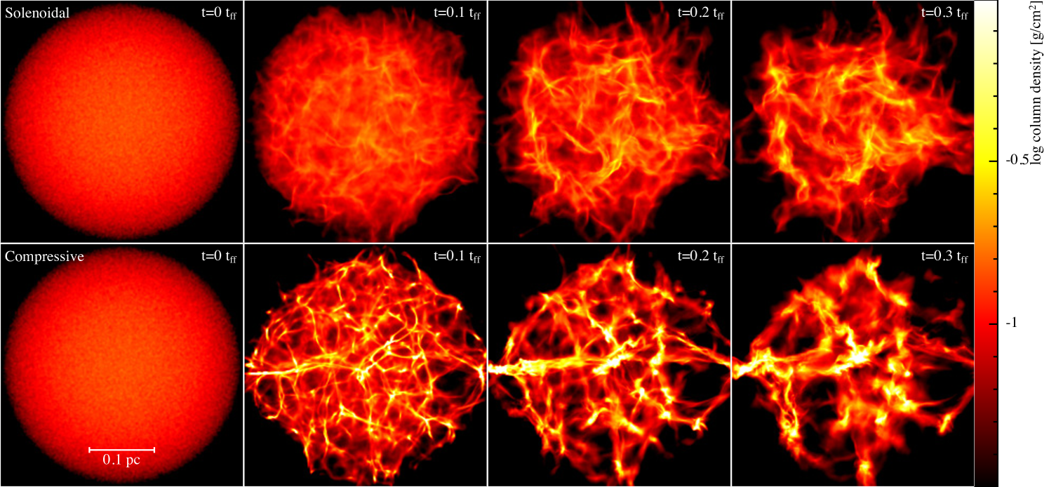
Figure 1 shows the evolution of column density from $t=0$ to $t=0.3t_{\rm ff}$ (left to right) in two representative calculations, using solenoidal driving (top, as in BBB03) and compressive driving (bottom). Shocks form quickly in both cases, due to the impulsive supersonic velocity field, but are stronger in the compressive case, driving the formation of large scale filaments after only $0.3t_{\mathrm{ff}}$. For the solenoidal case, $\nabla\cdot\mathbf{v}=0$ initially by definition, so there are no regions that initially promote collapse.

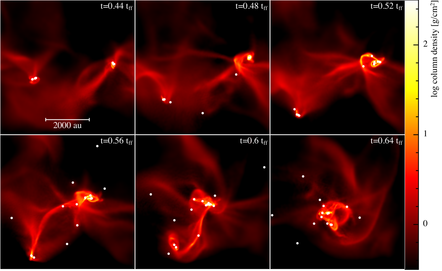
Figure 2 shows the subsequent small-scale fragmentation in the compressive cloud, with the first protostar formed after just $0.2t_{\rm ff}$. The process in all other clouds appears visually very similar. Gas flows into dense cores along filaments (e.g. Gómez & Vázquez-Semadeni, 2014; Smith et al., 2016; Federrath, 2016; Klassen et al., 2016), feeding young protostars via accretion discs. The process is chaotic and dynamical, with close encounters between stars resulting in the destruction of accretion discs, and the ejection of smaller mass objects. Bound systems form and get destroyed by interactions on a very short time-scale. The stars live in a competitive environment, where those that grow in mass quickly stay in the dense regions and accrete further material, whilst ejecting lower mass objects.

We computed the density PDFs by binning the particles into 2000 bins equally spaced between $-10<\log_{10}(\rho)<10$ in code units. We then computed the standard deviation, $\sigma_{\ln\rho}$ by fitting a log-normal distribution to the PDF (using scipy.optimize.curve_fit in Python). Note that the PDF computed in this way is mass, rather than volume-weighted. Both volume and mass-weighted PDFs are expected to be log-normal when the equation of state is approximately isothermal (Padoan et al., 1997b; Passot & Vázquez-Semadeni, 1998; Scalo et al., 1998; Nordlund & Padoan, 1999; Ostriker et al., 2001).

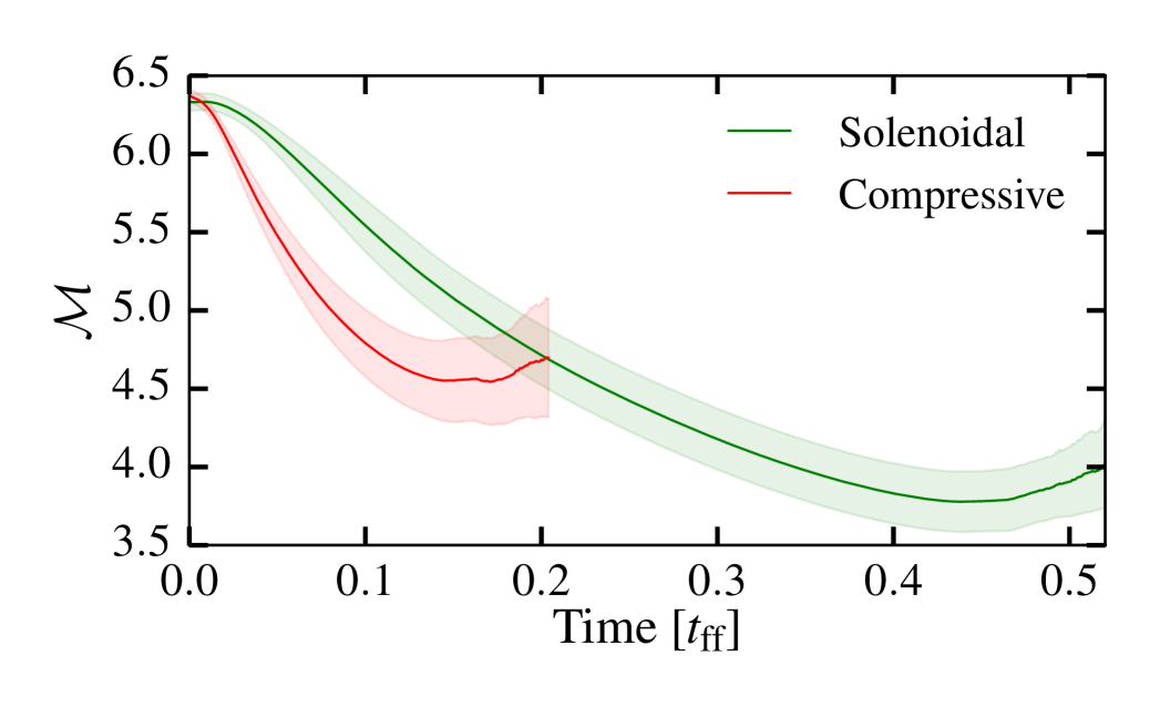
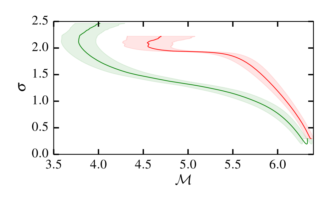
Figure 3 shows the time evolution of the (mass weighted) RMS Mach number, $\mathcal{M}$, (top panel) and standard deviation, $\sigma_{\ln\rho}$, (centre panel) for our entire set of calculations, with the solid lines showing the mean from the 7 different simulations for each type of velocity field and the shaded region shows the 1$\sigma$ standard deviation. The bottom panel shows the evolution in the $\mathcal{M}$-$\sigma_{\ln\rho}$ plane. In both the solenoidal and compressive clouds $\mathcal{M}$ decays with time due to the dissipation of energy by shocks, reaching a minimum before rising again once bound structures have formed.

Comparison of PDFs in decaying turbulence simulations is complicated by the time evolution of the velocity field. In our calculations the initial density field is uniform and the PDF thus develops in response to the initial turbulent velocity field. Since the clouds evolve on different time-scales, it is not particularly meaningful to compare their PDFs at the same time. Rather — for the purposes of our study — Equation 1 suggests that they should be compared at the same RMS Mach number $\mathcal{M}$ so that the only difference is from the different mixing parameters $b$.

The lower panel of Figure 3 shows that the initial collapse of the cloud roughly corresponds to $\sigma_{\ln\rho}\lesssim 2$. Once $\sigma_{\ln\rho}$ reaches this value $\mathcal{M}$ rises again once fragmentation begins. Also, the PDF is no longer log-normal. We thus use the time interval where $\sigma_{\ln\rho}<2$ to compare the density PDFs prior to the onset of star formation. The standard deviation of the PDFs is different not only at the same time early in the evolution of the cloud, but also at the same RMS Mach number.

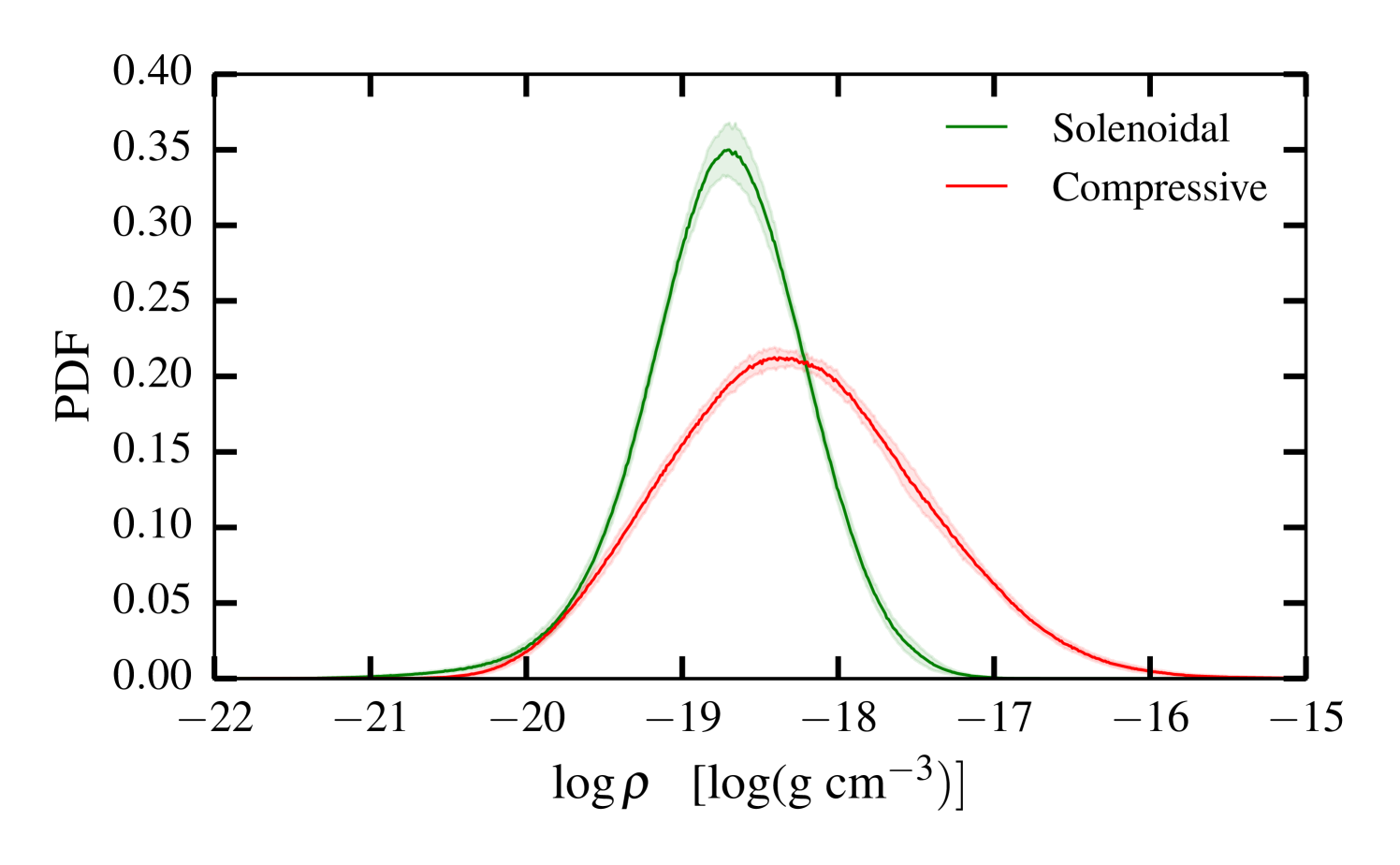
Figure 4 shows the resultant PDFs computed at the time when all calculations have the same RMS Mach number of $\mathcal{M}=5.5$, which is when $\sigma$ differs most between the simulations. The difference in the PDF produced by compressive vs. solenoidal driving is similar to that shown by (e.g.) Federrath et al. (2008) and Federrath et al. (2010), except that we show the mass-weighted version. Compressive driving produces a broadening of the PDF caused by the collision of stronger shocks which in turn create larger variations in the density field. This demonstrates that our different choices of impulsive driving indeed drive significant differences in the density PDF prior to star formation.

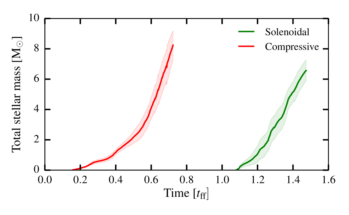
Figure 5 shows the total stellar mass as a function of time, measured by the mass in sink particles. The onset of star formation occurs at $t\approx 0.2t_{\rm ff}$ in the compressive case, compared to $t\approx 1.1t_{\rm ff}$ in the solenoidal case. Once star formation starts in each calculation, the rate at which material is converted to stars is higher by a factor of $\sim 2$ in the compressive clouds compared to the solenoidal cloud. The overall efficiency of star formation is similar in both types of calculation over the time we have continued the simulations, with $\approx 15$% of the gas mass converted to stars. However, the efficiency is higher on an absolute scale since this occurs over a shorter timescale in the compressive case. Also, the end of the simulations does not mark the end of the star formation process since the mass in stars continues to increase.

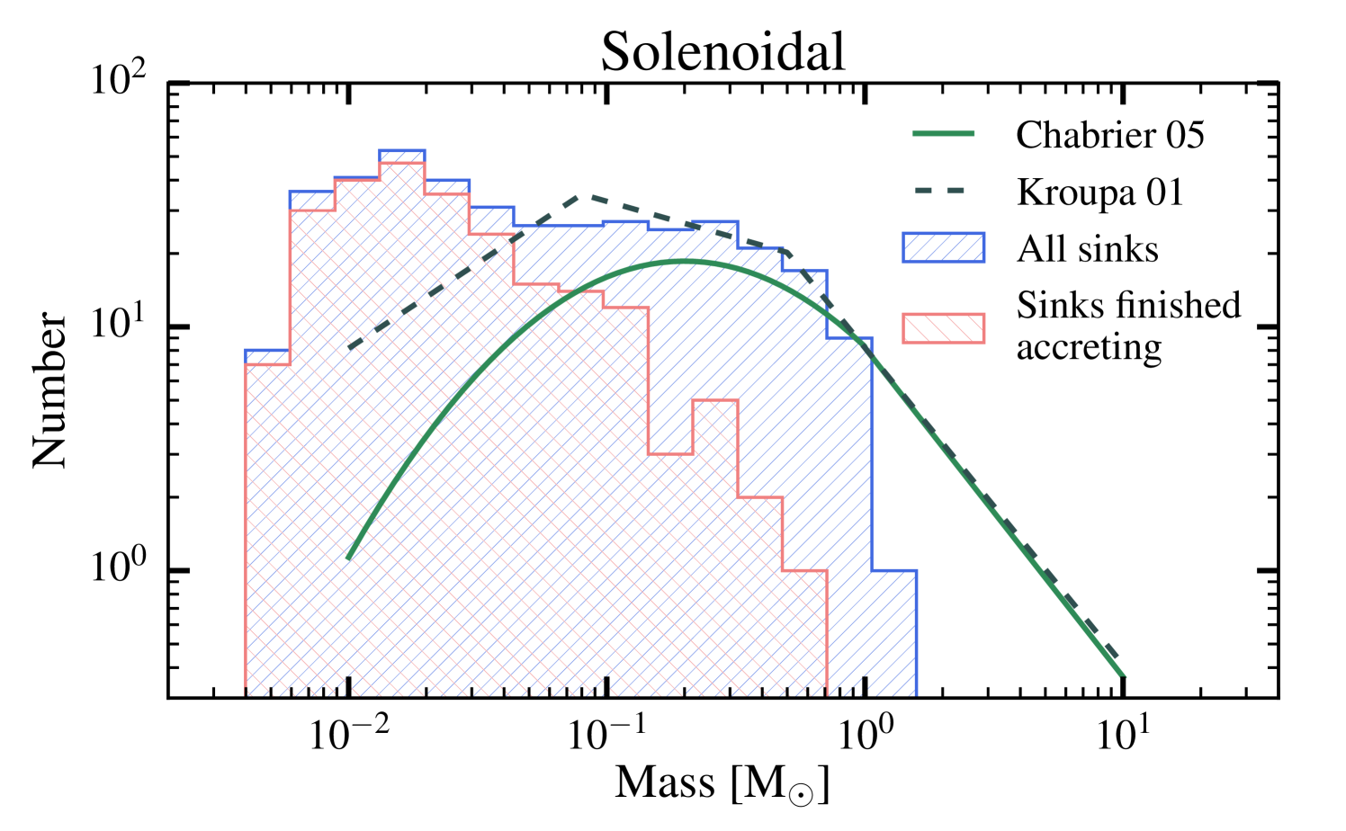
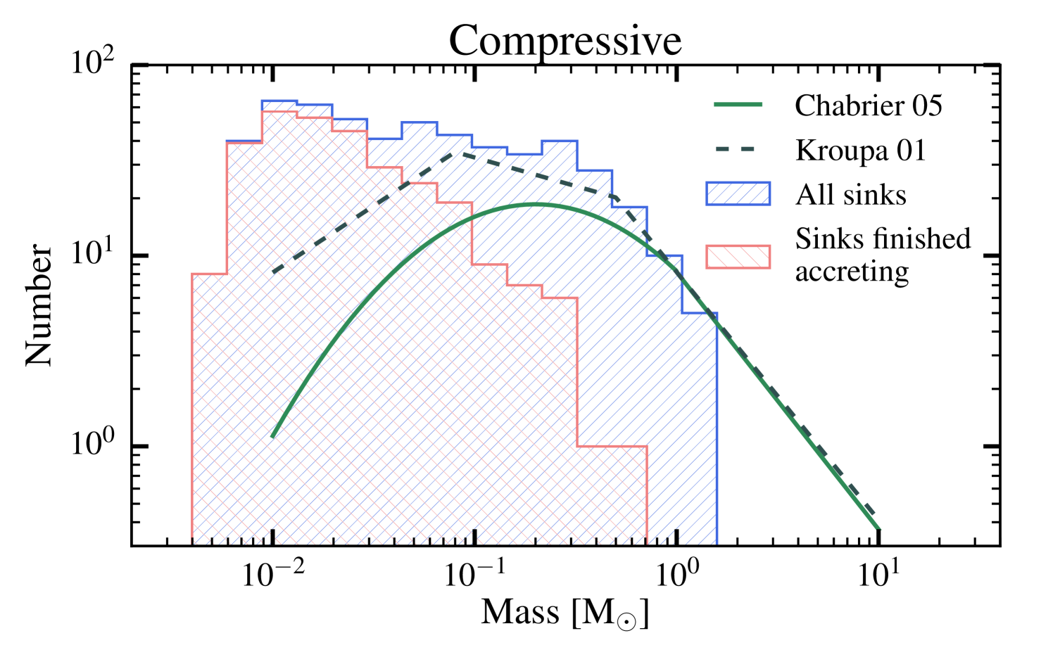
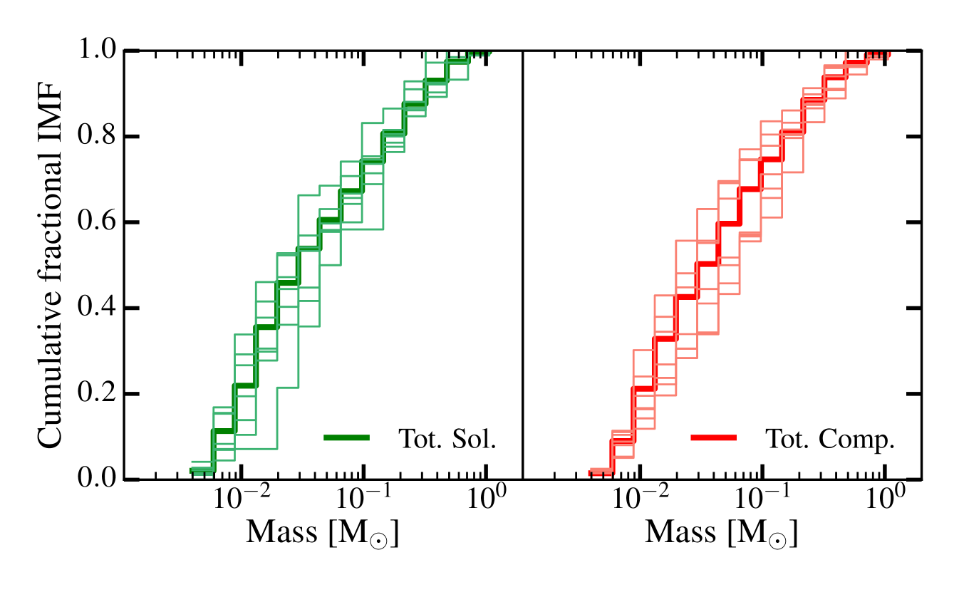
Figure 6 shows the IMFs from our simulations, combining all 7 realisations with solenoidal (left) and compressive driving (right), with the cumulative IMFs shown in Figure 7. The IMFs of stars that have finished accreting (235 of 388 and 298 of 533 sinks for solenoidal and compressive, respectively) are shown in red, while the IMF of all stars is shown in blue. The lowest mass possible in our calculations is $\approx 0.005\text{ M}_{\odot}$ from the opacity limit for fragmentation, which sets the low-mass cutoff. The IMFs appear similar to those shown in BBB03 but with better statistics because of our multiple realisations. Our IMFs are also similar to those found by Bate (2009a) from one calculation of a 500 $\text{M}_{\odot}$ cloud. In particular, we observe the statistically significant excess in low mass stars and brown dwarfs compared to the Kroupa (2001) and Chabrier (2005) IMFs (dashed and solid lines, respectively) that occurs when a barotropic equation of state is employed (e.g. Bate, 2009a, b).

There is no obvious difference between the IMFs produced by the different types of driving. Statistics confirm this — a Kolmogorov-Smirnov test gives a p-value of 0.71 between the two distributions when considering all sink particles, and a p-value of 0.98 when considering only sinks that have finished accreting. This means we cannot reject the hypothesis that the samples come from the same underlying distribution. Thus, while the type of driving changes the density PDF, the resultant IMFs are indistinguishable.

References

- Alves et al. (2007) Alves J., Lombardi M., Lada C. J., 2007, A&A, 462, L17
- Ballesteros-Paredes et al. (2006) Ballesteros-Paredes J., Gazol A., Kim J., Klessen R. S., Jappsen A.-K., Tejero E., 2006, ApJ, 637, 384
- Bastian et al. (2010) Bastian N., Covey K. R., Meyer M. R., 2010, ARA&A, 48, 339
- Bate (2009a) Bate M. R., 2009a, MNRAS, 392, 590
- Bate (2009b) Bate M. R., 2009b, MNRAS, 392, 1363
- Bate (2009c) Bate M. R., 2009c, MNRAS, 397, 232
- Bate (2012) Bate M. R., 2012, MNRAS, 419, 3115
- Bate & Bonnell (2005) Bate M. R., Bonnell I. A., 2005, MNRAS, 356, 1201
- Bate & Burkert (1997) Bate M. R., Burkert A., 1997, MNRAS, 288, 1060
- Bate et al. (1995) Bate M. R., Bonnell I. A., Price N. M., 1995, MNRAS, 277, 362
- Bate et al. (2003) Bate M. R., Bonnell I. A., Bromm V., 2003, MNRAS, 339, 577
- Bertelli Motta et al. (2016) Bertelli Motta C., Clark P. C., Glover S. C. O., Klessen R. S., Pasquali A., 2016, MNRAS, 462, 4171
- Bonnell et al. (1997) Bonnell I. A., Bate M. R., Clarke C. J., Pringle J. E., 1997, MNRAS, 285, 201
- Chabrier (2003) Chabrier G., 2003, PASP, 115, 763
- Chabrier (2005) Chabrier G., 2005, in Corbelli E., Palla F., Zinnecker H., eds, Astrophysics and Space Science Library Vol. 327, The IMF 50 Years Later. p. 41
- Chabrier & Hennebelle (2010) Chabrier G., Hennebelle P., 2010, ApJ, 725, L79
- Commerçon et al. (2010) Commerçon B., Hennebelle P., Audit E., Chabrier G., Teyssier R., 2010, A&A, 510, L3
- Dubinski et al. (1995) Dubinski J., Narayan R., Phillips T. G., 1995, ApJ, 448, 226
- Elmegreen & Scalo (2004) Elmegreen B. G., Scalo J., 2004, ARA&A, 42, 211
- Enoch et al. (2008) Enoch M. L., Evans II N. J., Sargent A. I., Glenn J., Rosolowsky E., Myers P., 2008, ApJ, 684, 1240
- Federrath (2016) Federrath C., 2016, MNRAS, 457, 375
- Federrath et al. (2008) Federrath C., Klessen R. S., Schmidt W., 2008, ApJ, 688, L79
- Federrath et al. (2010) Federrath C., Roman-Duval J., Klessen R. S., Schmidt W., Mac Low M.-M., 2010, A&A, 512, A81
- Girichidis et al. (2011) Girichidis P., Federrath C., Banerjee R., Klessen R. S., 2011, MNRAS, 413, 2741
- Gómez & Vázquez-Semadeni (2014) Gómez G. C., Vázquez-Semadeni E., 2014, ApJ, 791, 124
- Goodwin et al. (2008) Goodwin S. P., Nutter D., Kroupa P., Ward-Thompson D., Whitworth A. P., 2008, A&A, 477, 823
- Guszejnov & Hopkins (2015) Guszejnov D., Hopkins P. F., 2015, MNRAS, 450, 4137
- Heitsch et al. (2001) Heitsch F., Mac Low M.-M., Klessen R. S., 2001, ApJ, 547, 280
- Hennebelle & Chabrier (2008) Hennebelle P., Chabrier G., 2008, ApJ, 684, 395
- Hennebelle & Chabrier (2009) Hennebelle P., Chabrier G., 2009, ApJ, 702, 1428
- Heyer & Brunt (2004) Heyer M. H., Brunt C. M., 2004, ApJ, 615, L45
- Hopkins (2012) Hopkins P. F., 2012, MNRAS, 423, 2037
- Johnstone et al. (2000) Johnstone D., Wilson C. D., Moriarty-Schieven G., Joncas G., Smith G., Gregersen E., Fich M., 2000, ApJ, 545, 327
- Kainulainen et al. (2009) Kainulainen J., Beuther H., Henning T., Plume R., 2009, A&A, 508, L35
- Klassen et al. (2016) Klassen M., Pudritz R. E., Kirk H., 2016, preprint, (arXiv:1605.08835)
- Klessen (2000) Klessen R. S., 2000, ApJ, 535, 869
- Kritsuk et al. (2007) Kritsuk A. G., Norman M. L., Padoan P., Wagner R., 2007, ApJ, 665, 416
- Kroupa (2001) Kroupa P., 2001, MNRAS, 322, 231
- Krumholz & McKee (2005) Krumholz M. R., McKee C. F., 2005, ApJ, 630, 250
- Krumholz et al. (2010) Krumholz M. R., Cunningham A. J., Klein R. I., McKee C. F., 2010, ApJ, 713, 1120
- Krumholz et al. (2012) Krumholz M. R., Klein R. I., McKee C. F., 2012, ApJ, 754, 71
- Lada et al. (2008) Lada C. J., Muench A. A., Rathborne J., Alves J. F., Lombardi M., 2008, ApJ, 672, 410
- Larson (1981) Larson R. B., 1981, MNRAS, 194, 809
- Lemaster & Stone (2008) Lemaster M. N., Stone J. M., 2008, ApJ, 682, L97
- Lodato & Price (2010) Lodato G., Price D. J., 2010, MNRAS, 405, 1212
- Lomax et al. (2015) Lomax O., Whitworth A. P., Hubber D. A., 2015, MNRAS, 449, 662
- Lombardi et al. (2006) Lombardi M., Alves J., Lada C. J., 2006, A&A, 454, 781
- Lombardi et al. (2008) Lombardi M., Lada C. J., Alves J., 2008, A&A, 489, 143
- Lombardi et al. (2010) Lombardi M., Lada C. J., Alves J., 2010, A&A, 512, A67
- Low & Lynden-Bell (1976) Low C., Lynden-Bell D., 1976, MNRAS, 176, 367
- Luhman & Rieke (1999) Luhman K. L., Rieke G. H., 1999, ApJ, 525, 440
- Molina et al. (2012) Molina F. Z., Glover S. C. O., Federrath C., Klessen R. S., 2012, MNRAS, 423, 2680
- Motte et al. (1998) Motte F., Andre P., Neri R., 1998, A&A, 336, 150
- Myers et al. (2014) Myers A. T., Klein R. I., Krumholz M. R., McKee C. F., 2014, MNRAS, 439, 3420
- Nordlund & Padoan (1999) Nordlund Å. K., Padoan P., 1999, in Franco J., Carraminana A., eds, Interstellar Turbulence. Cambridge; CUP, p. 218
- Nutter & Ward-Thompson (2007) Nutter D., Ward-Thompson D., 2007, MNRAS, 374, 1413
- Offner et al. (2009) Offner S. S. R., Klein R. I., McKee C. F., Krumholz M. R., 2009, ApJ, 703, 131
- Ostriker et al. (1999) Ostriker E. C., Gammie C. F., Stone J. M., 1999, ApJ, 513, 259
- Ostriker et al. (2001) Ostriker E. C., Stone J. M., Gammie C. F., 2001, ApJ, 546, 980
- Padoan & Nordlund (2002) Padoan P., Nordlund Å., 2002, ApJ, 576, 870
- Padoan et al. (1997a) Padoan P., Nordlund A., Jones B. J. T., 1997a, MNRAS, 288, 145
- Padoan et al. (1997b) Padoan P., Jones B. J. T., Nordlund A. P., 1997b, ApJ, 474, 730
- Passot & Vázquez-Semadeni (1998) Passot T., Vázquez-Semadeni E., 1998, Phys. Rev. E, 58, 4501
- Price (2007) Price D. J., 2007, PASA, 24, 159
- Price (2012) Price D. J., 2012, J. Comp. Phys., 231, 759
- Price & Bate (2008) Price D. J., Bate M. R., 2008, MNRAS, 385, 1820
- Price & Bate (2009) Price D. J., Bate M. R., 2009, MNRAS, 398, 33
- Price & Federrath (2010) Price D. J., Federrath C., 2010, MNRAS, 406, 1659
- Price et al. (2011) Price D. J., Federrath C., Brunt C. M., 2011, ApJ, 727, L21
- Rathborne et al. (2009) Rathborne J. M., et al., 2009, ApJ, 699, 742
- Rees (1976) Rees M. J., 1976, MNRAS, 176, 483
- Scalo et al. (1998) Scalo J., Vazquez-Semadeni E., Chappell D., Passot T., 1998, ApJ, 504, 835
- Smith et al. (2008) Smith R. J., Clark P. C., Bonnell I. A., 2008, MNRAS, 391, 1091
- Smith et al. (2009) Smith R. J., Clark P. C., Bonnell I. A., 2009, MNRAS, 396, 830
- Smith et al. (2016) Smith R. J., Glover S. C. O., Klessen R. S., Fuller G. A., 2016, MNRAS, 455, 3640
- Testi & Sargent (1998) Testi L., Sargent A. I., 1998, ApJ, 508, L91
- Tilley & Pudritz (2007) Tilley D. A., Pudritz R. E., 2007, MNRAS, 382, 73
- Vazquez-Semadeni (1994) Vazquez-Semadeni E., 1994, ApJ, 423, 681
- Vázquez-Semadeni et al. (2005) Vázquez-Semadeni E., Kim J., Ballesteros-Paredes J., 2005, ApJ, 630, L49
- Zuckerman & Evans (1974) Zuckerman B., Evans II N. J., 1974, ApJ, 192, L149