Domain decomposition and partitioning methods for mixed finite element discretizations of the Biot system of poroelasticity
Abstract
We develop non-overlapping domain decomposition methods for the Biot system of poroelasticity in a mixed form. The solid deformation is modeled with a mixed three-field formulation with weak stress symmetry. The fluid flow is modeled with a mixed Darcy formulation. We introduce displacement and pressure Lagrange multipliers on the subdomain interfaces to impose weakly continuity of normal stress and normal velocity, respectively. The global problem is reduced to an interface problem for the Lagrange multipliers, which is solved by a Krylov space iterative method. We study both monolithic and split methods. In the monolithic method, a coupled displacement-pressure interface problem is solved, with each iteration requiring the solution of local Biot problems. We show that the resulting interface operator is positive definite and analyze the convergence of the iteration. We further study drained split and fixed stress Biot splittings, in which case we solve separate interface problems requiring elasticity and Darcy solves. We analyze the stability of the split formulations. Numerical experiments are presented to illustrate the convergence of the domain decomposition methods and compare their accuracy and efficiency.
Keywords: domain decomposition, poroelasticity, Biot system, splitting methods, mixed finite elements
1 Introduction
In this paper we study several non-overlapping domain decomposition methods for the Biot system of poroelasticity [14], which models the flow of a viscous fluid through a poroelastic medium along with the deformation of the medium. Such flow occurs in many geophysics phenomena like earthquakes, landslides, and flow of oil inside mineral rocks and plays a key role in engineering applications such as hydrocarbon extraction through hydraulic or thermal fracturing. We use the classical Biot system of poroelasticity with the quasi-static assumption, which is particularly relevant in geoscience applications. The model consists of an equilibrium equation for the solid medium and a mass balance equation for the flow of the fluid through the medium. The system is fully coupled, with the fluid pressure contributing to the solid stress and the divergence of the solid displacement affecting the fluid content.
The numerical solution of the Biot system has been extensively studied in the literature. Various formulations have been considered, including two-field displacement–pressure formulations [27, 45, 51], three-field displacement–pressure–Darcy velocity formulations [48, 52, 62, 32, 41, 60, 49, 59], and three-field displacement–pressure–total pressure formulations [42, 47]. More recently, fully-mixed formulations of the Biot system have been studied. In [61], a four-field stress–displacement–pressure–Darcy velocity mixed formulation is developed. A posteriori error estimates for this formulation are obtained in [2]. In [39], a weakly symmetric stress–displacement–rotation elasticity formulation is considered, which is coupled with a mixed pressure–Darcy velocity flow formulation. Fully-mixed finite element approximations carry the advantages of local mass and momentum conservation, direct computation of the fluid velocity and the solid stress, as well as robustness and locking-free properties with respect to the physical parameters. Mixed finite element (MFE) methods can also handle discontinuous full tensor permeabilities and Lamé coefficients that are typical in subsurface flows. In our work we focus on the five-field weak-stress-symmetry formulation from [39], since weakly symmetric MFE methods for elasticity allow for reduced number of degrees of freedom. Moreover, a multipoint stress–multipoint flux mixed finite element approximation for this formulation has been recently developed in [7], which can be reduced to a positive definite cell-centered scheme for pressure and displacement only, see also a related finite volume method in [46]. While our domain decomposition methods are developed for the weakly symmetric formulation from [39], the analysis carries over in a straightforward way to the strongly symmetric formulation from [61].
Discretizations of the Biot system of poroelasticity for practical applications typically result in large algebraic systems of equations. The efficient solution of these systems is critical for the ability of the numerical method to provide the desired resolution. In this work we focus on non-overlapping domain decomposition methods [57, 50]. These methods split the computational domain into multiple non-overlapping subdomains with algebraic systems of lower complexity that are easier to solve. A global problem enforcing appropriate interface conditions is solved iteratively to recover the global solution. This approach naturally leads to scalable parallel algorithms. Despite the abundance of works on discretizations of the Biot system, there have been very few results on domain decomposition methods for this problem. In [28], a domain decomposition method using mortar elements for coupling the poroelastic model with an elastic model in an adjacent region is presented. In that work, the Biot region is not decomposed into subdomains. In [26, 25], an iterative coupling method is employed for a two-field displacement–pressure formulation, and classical domain decomposition techniques are applied separately for the elasticity and flow equations. A monolithic domain decomposition method for the two-field formulation of poroelasticity combining primal and dual variables is developed in [31]. To the best of our knowledge, domain decomposition methods for mixed formulations of poroelasticity have not been studied in the literature.
In this paper we study both monolithic and split non-overlapping domain decomposition methods for the five-field fully mixed formulation of poroelasticity with weak stress symmetry from [39, 7]. Monolithic methods require solving the coupled Biot system, while split methods only require solving elasticity and flow problems separately. Both methods have advantages and disadvantages. Monolithic methods involve solving larger and possibly ill-conditioned algebraic systems, but may be better suitable for problems with strong coupling between flow and mechanics, in which case split or iterative coupling methods may suffer from stability or convergence issues and require sufficiently small time steps. Our methods are motivated by the non-overlapping domain decomposition methods for MFE discretizations of Darcy flow developed in [29, 22, 8] and the non-overlapping domain decomposition methods for MFE discretizations of elasticity developed recently in [35].
In the first part of the paper we develop a monolithic domain decomposition method. We employ a physically heterogeneous Lagrange multiplier vector consisting of displacement and pressure variables to impose weakly the continuity of the normal components of stress and velocity, respectively. The algorithm involves solving at each time step an interface problem for this Lagrange multiplier vector. We show that the interface operator is positive definite, although it is not symmetric in general. As a result, a Krylov space solver such as GMRES can be employed for the solution of the interface problem. Each iteration requires solving monolithic Biot subdomain problems with specified Dirichlet data on the interfaces, which can be done in parallel. We establish lower and upper bounds on the spectrum of the interface operator, which allows us to perform analysis of the convergence of the GMRES iteration using field-of-values estimates.
In the second part of the paper we study split domain decomposition methods for the Biot system. Split or iterative coupling methods for poroelasticity have been extensively studied due to their computational efficiency. Four widely used sequential methods are drained split, undrained split, fixed stress split, and fixed strain split. Decoupling methods are prone to stability issues and a detailed stability analysis of the aforementioned schemes using finite volume methods can be found in [36, 37], see also [20] for stability analysis of several split methods using displacement–pressure finite element discretizations. Iterative coupling methods are based on similar splittings and involve iterating between the two sub-systems until convergence. Convergence for non-mixed finite element methods is analyzed in [44], while convergence for a four-field mixed finite element discretization is studied in [63]. An accelerated fixed stress splitting scheme for a generalized non-linear consolidation of unsaturated porous medium is studied in [18]. Studies of the optimization and acceleration of the fixed stress decoupling method for the Biot consolidation model, including techniques such as multirate or adaptive time stepping and parallel-in-time splittings have been presented in [1, 13, 17, 56, 3].
In our work we consider drained split (DS) and fixed stress (FS) decoupling methods in conjunction with non-overlapping domain decomposition. In particular, at each time step we solve sequentially an elasticity and a flow problem in the case of DS or a flow and an elasticity problem in the case of FS splitting. We perform stability analysis for the two splittings using energy estimates and show that they are both unconditionally stable with respect to the time step and the physical parameters. We then employ separate non-overlapping domain decomposition methods for each of the decoupled problems, using the methods developed in [29, 8] for flow and [35] for mechanics.
In the numerical section we present several computational experiments designed to verify and compare the accuracy, stability, and computational efficiency of the three domain decomposition methods for the Biot system of poroelasticity. In particular, we study the discretization error and the number of interface iterations, as well as the effect of the number of subdomains. We also illustrate the performance of the methods for a physically realistic heterogeneous problem with data taken from the Society of Petroleum Engineers 10th Comparative Solution Project.
The rest of the paper is organized as follows. In Section 2 we introduce the mathematical model and its MFE discretization. The monolithic domain decomposition method is developed and analyzed in Section 3. In Section 4 we perform stability analysis of the DS and FS decoupling methods and present the DS and FS domain decomposition methods. The numerical experiments are presented in Section 5, followed by conclusions in Section 6.
2 Model problem and its MFE discretization
Let , be a simply connected domain occupied by a linearly elastic porous body. We use the notation , , and for the spaces of matrices, symmetric matrices, and skew-symmetric matrices respectively, all over the field of real numbers, respectively. Throughout the paper, the divergence operator is the usual divergence for vector fields, which produces vector field when applied to matrix field by taking the divergence of each row. For a domain , the inner product and norm for scalar, vector, or tensor valued functions are denoted and , respectively. The norms and seminorms of the Hilbert spaces are denoted by and , respectively. We omit in the subscript if . For a section of the domain or element boundary we write and for the inner product (or duality pairing) and norm, respectively. We will also use the spaces
equipped with the norm
The partial derivative operator with respect to time, , is often abbreviated to . Finally, denotes a generic positive constant that is independent of the discretization parameters and .
Given a vector field representing body forces and a source term , the quasi-static Biot system of poroelasticity is [14]:
| (2.1) | |||||
| (2.2) | |||||
| (2.3) |
where is the displacement, is the fluid pressure, is the Darcy velocity, and is the poroelastic stress, defined as
| (2.4) |
Here is the identity matrix, is the Biot-Willis constant, and is the elastic stress satisfying the stress-strain relationship
| (2.5) |
where is the compliance tensor, which is a symmetric, bounded and uniformly positive definite linear operator acting from , extendible to . In the special case of homogeneous and isotropic body, is given by,
| (2.6) |
where and are the Lamé coefficients. In this case, . Finally, stands for the permeability tensor, which is symmetric, bounded, and uniformly positive definite, and is the mass storativity. To close the system, we impose the boundary conditions
| on | , | (2.7) | |||||||
| on | , | (2.8) |
where and is the outward unit normal vector field on , along with the initial condition in . Compatible initial data for the rest of the variables can be obtained from (2.1) and (2.2) at . Well posedness analysis for this system can be found in [53].
We consider a mixed variational formulation for (2.1)–(2.8) with weak stress symmetry, following the approach in [39]. The motivation is that MFE elasticity spaces with weakly symmetric stress tend to have fewer degrees of freedom than strongly symmetric MFE spaces. Moreover, in a recent work, a multipoint stress–multipoint flux mixed finite element method has been developed for this formulation that reduces to a positive definite cell-centered scheme for pressure and displacement only [7]. Nevertheless, the domain decomposition methods in this paper can be employed for strongly symmetric stress formulations, with the analysis carrying over in a straightforward way. We introduce a rotation Lagrange multiplier , which is used to impose weakly symmetry of the stress tensor . We rewrite (2.5) as
| (2.9) |
Combining (2.5) and (2.4) gives , which can be used to rewrite (2.3) as
| (2.10) |
The combination of (2.9), (2.1), (2.2), and (2.10), along with the boundary conditions (2.7)–(2.8), leads to the variational formulation: find such that and for a.e. ,
| (2.11) | ||||
| (2.12) | ||||
| (2.13) | ||||
| (2.14) | ||||
| (2.15) |
where
It was shown in [7] that the system (2.11)–(2.15) is well posed.
Next, we present the MFE discretization of (2.11)–(2.15). For simplicity we assume that is a Lipshicz polygonal domain. Let be a shape-regular quasi-uniform finite element partition of , consisting of simplices or quadrilaterals, with . The MFE method for solving (2.11)–(2.15) is: find such that, for a.e. ,
| (2.16) | ||||
| (2.17) | ||||
| (2.18) | ||||
| (2.19) | ||||
| (2.20) |
with discrete initial data obtained as the elliptic projection of the continuous initial data. Here is a collection of suitable finite element spaces. In particular, could be chosen from any of the known stable triplets for linear elasticity with weak stress symmetry, e.g. [55, 5, 9, 10, 11, 21, 30, 15, 16, 24, 6, 40], satisfying the inf-sup condition
| (2.21) |
For the flow part, could be chosen from any of the known stable velocity-pressure pairs of MFE spaces such as the Raviart-Thomas () or Brezzi-Douglas-Marini () spaces, see [19], satisfying the inf-sup condition
| (2.22) |
3 Monolithic domain decomposition method
Let be a union of non-overlapping shape-regular polygonal subdomains, where each subdomain is a union of elements of . Let and denote the interior subdomain interfaces. Denote the restriction of the spaces , , , , and to by , , , , and , respectively. Let be a finite element partition of obtained from the trace of , and let be a unit normal vector on with an arbitrarily fixed direction. In the domain decomposition formulation we utilize a vector Lagrange multiplier approximating the displacement and the pressure on the interface and used to impose weakly the continuity of the normal components of the poroelastic stress tensor and the velocity vector , respectively. We define the Lagrange multiplier space on and as follows:
The domain decomposition formulation for the mixed Biot problem in a semi-discrete form reads as follows: for , find such that, for a.e. ,
| (3.1) | ||||
| (3.2) | ||||
| (3.3) | ||||
| (3.4) | ||||
| (3.5) | ||||
| (3.6) | ||||
| (3.7) | ||||
where is the outward unit normal vector field on . We note that both the elasticity and flow subdomain problems in the above method are of Dirichlet type. It is easy to check that (3.1)–(3.7) is equivalent to the global formulation (2.16)–(2.20) with .
3.1 Time discretization
For time discretization we employ the backward Euler method. Let , , , be a uniform partition of . The fully discrete problem corresponding to (3.1)–(3.7) reads as follows: for and , find such that:
| (3.8) | ||||
| (3.9) | ||||
| (3.10) | ||||
| (3.11) | ||||
| (3.12) | ||||
| (3.13) | ||||
| (3.14) | ||||
3.2 Time-differentiated elasticity formulation
In the monolithic domain decomposition method we will utilize a related formulation in which the first elasticity equation is differentiated in time. The reason for this will become clear in the analysis of the resulting interface problem. We introduce new variables and representing the time derivatives of the displacement and the rotation, respectively. The time-differentiated equation (2.11) is
The semi-discrete equation (2.16) is replaced by
We note that the original variables and can be recovered easily from the solution of the time-differentiated problem. In particular, given compatible initial data , , that satisfy (2.16), the expressions
provide a solution to (2.16) at any .
In the domain decomposition formulation we now consider the Lagrange multiplier , where approximates the trace of on . Then the semi-discrete domain decomposition equation (3.1) is replaced by
Finally, the fully discrete equation (3.8) is replaced by
| (3.15) | ||||
The original variables can be recovered from
| (3.16) |
3.3 Reduction to an interface problem
The non-overlapping domain decomposition algorithm for the solution of (3.15), (3.9)–(3.14) at each time step is based on reducing it to an interface problem for the Lagrange multiplier . To this end, we introduce two sets of complementary subdomain problems. The first set of problems reads as follows: for , find such that
| (3.17) | ||||
| (3.18) | ||||
| (3.19) | ||||
| (3.20) | ||||
| (3.21) | ||||
These subdomain problems have zero Dirichlet data on the interfaces and incorporate the true source terms and and outside boundary conditions and , as well as initial data and .
The second problem set reads as follows: given , for , find such that:
| (3.22) | ||||
| (3.23) | ||||
| (3.24) | ||||
| (3.25) | ||||
| (3.26) | ||||
These problems have as Dirichlet interface data, along with zero source terms, zero outside boundary conditions, and zero data from the previous time step.
3.4 Analysis of the interface problem
We next show that the interface bilinear form is positive definite, which implies that the interface problem (3.29) is well-posed and can be solved using a suitable Krylov space method such as GMRES. We further obtain bounds on the spectrum of and establish rate of convergence for GMRES. We start by obtaining an expression for in terms of the subdomain bilinear forms.
Proposition 3.1.
For , the interface bilinear form can be expressed as
| (3.30) |
Proof.
Remark 3.2.
Recalling the properties of and , there exist constants and such that
| (3.31) | |||
| (3.32) |
We will also utilize suitable mixed interpolants in the finite element spaces and . It is shown in [35] that there exists an interpolant for any such that for all , , , and ,
| (3.33) |
and
| (3.34) |
For the Darcy problem we use the canonical mixed interpolant [19], such that for all , , and ,
| (3.35) |
and
| (3.36) |
Lemma 3.2.
The interface bilinear form is positive definite over .
Proof.
Using the representation of the interface bilinear form (3.30), we get
| (3.37) |
which, combined with (3.31)–(3.32), gives , and hence is positive semidefinite. We next show that implies . We use a two-part argument to control separately and . Let be a domain adjacent to such that and let be the solution of the auxiliary elasticity problem
Elliptic regularity [23] implies that for some , and therefore the mixed interpolant is well defined. Taking in (3.22) and using (3.33) and (3.34) gives
| (3.38) |
where in the last inequality we used the elliptic regularity bound [23]
| (3.39) |
Using the representation of the interface bilinear form (3.30), we obtain
| (3.40) |
Next, consider an adjacent subdomain such that . Let be the solution to
Taking in (3.22) and using (3.33) gives
where in the first inequality we used (3.34) and the trace inequality [43]
and for the second inequality we used the representation (3.30) and the bound from (3.40), along with the elliptic regularity bound (3.39). Iterating over all subdomains in a similar fashion results in
| (3.41) |
The argument for is similar. We start with a subdomain adjacent to such that and let be the solution of the auxiliary flow problem
| (3.42) | |||
| (3.43) | |||
| (3.44) |
Taking in (3.25) and using (3.35), (3.36), and elliptic regularity similar to (3.39) gives
which, together with (3.30) implies
Iterating over all subdomains in a way similar to the argument for , we obtain
| (3.45) |
A combination of (3.41) and (3.45) implies that is positive definite on . ∎
Theorem 3.3.
There exist positive constants and independent of and such that
| (3.46) |
In addition, there exist positive constants and independent of , , and such that
| (3.47) |
Proof.
The left inequality in (3.46) and (3.47) follows from (3.41) and (3.45). To prove the right inequality, we use the definition of the interface operator (3.27) to obtain
| (3.48) |
where for the second inequality we used the discrete trace inequality for finite element functions ,
| (3.49) |
and the last inequality follows from (3.37). We note that the constant in the last inequality depends on . This implies the right inequality in (3.46).
To obtain the right inequality in (3.47) with a constant independent of , we use the inf-sup condition (2.22) and (3.25):
| (3.50) |
where the last inequality uses (3.49). Combining (3.50) with the next to last inequality in (3.48) and using (3.37), we get:
using Young’s inequality in the last inequality. Taking sufficiently small implies the right inequality in (3.47). ∎
Theorem 3.3 provides upper and lower bounds on the field of values of the interface operator, which can be used to estimate the convergence of the interface GMRES solver. In particular, let be the -th residual of the GMRES iteration for solving the interface problem (3.29). Define , where denotes the Euclidean vector norm. The following corollary to Theorem 3.3 follows from the field-of-values analysis in [54].
Corollary 3.4.
4 Split methods
In this section, we consider two popular splitting methods to decouple the fully coupled poroelastic problem, namely the drained split (DS) and fixed stress (FS) methods [36, 37]. We show, using energy bounds, that these two methods are unconditionally stable in our MFE formulation. We then define, at each time step, a domain decomposition algorithm for the flow and mechanics equations separately. Domain decomposition techniques for the flow [29] and mechanics [35] components have already been studied in previous works.
4.1 Drained split
The DS method consists of solving the mechanics problem first, with the value of pressure from the previous time step. Afterward, the flow problem is solved using the new values of the stress tensor. The DS method for the classical Biot formulation of poroelasticity is known to require certain conditions on the parameters for stability [36]. In the setting of our mixed formulation, we show that this is not necessary and the method is unconditionally stable, see also [63]. For simplicity, we do the analysis with zero source terms.
The DS method results in the problem: for , find such that
| (4.1) | ||||
| (4.2) | ||||
| (4.3) |
and
| (4.4) | ||||
| (4.5) |
where (4.1)–(4.4) hold for with , and (4.5) holds for . We note that solving (4.1)–(4.4) for provides initial data , , , and .
4.1.1 Stability analysis for drained split
The following theorem shows that the drained split scheme is unconditionally stable.
Theorem 4.1.
Proof.
We subtract two successive time steps for equations (4.1)–(4.4), obtaining, for ,
| (4.6) | ||||
| (4.7) | ||||
| (4.8) | ||||
| (4.9) |
Taking , and in (4.6)–(4.8) and summing gives
implying
| (4.10) |
Taking in (4.9) and in (4.5) and summing results in
which, combined with (4.10), implies
Summing over from 0 to for any and using that gives
We note that the second and fourth terms are suboptimal with respect to . Neglecting these terms and using (3.32), we obtain
| (4.11) |
To obtain control on independent of , we use the inf-sup condition (2.22) and (4.4):
| (4.12) |
Taking , , and in (4.1)–(4.3) gives
| (4.13) |
For the stability of and , the inf-sup condition (2.21) combined with (4.1) gives:
| (4.14) |
A combination of bounds (4.11)–(4.14) completes the proof of the theorem.
∎
4.2 Fixed stress
The FS decoupling method solves the flow problem first, with the value of fixed from the previous time step. After that, the mechanics problem is solved using the new values of the pressure as data [37]. We again assume in the analysis zero source terms for simplicity. The method is: for , find such that
| (4.15) | ||||
| (4.16) | ||||
and
| (4.17) | ||||
| (4.18) | ||||
| (4.19) |
where the equations (4.15) and (4.17)–(4.19) hold for and (4.16) holds for with . Solving (4.15) and (4.17)–(4.19) for provides initial data , , , and .
4.2.1 Stability analysis for fixed stress
The following theorem shows that the fixed stress scheme is unconditionally stable.
Theorem 4.2.
Proof.
The proof is similar to that of the drained split scheme. Taking the difference of two successive time steps for equations (4.17)–(4.19) and (4.15), we obtain, for ,
| (4.20) | ||||
| (4.21) | ||||
| (4.22) | ||||
| (4.23) | ||||
Taking , and in (4.20)–(4.22) and adding the equations results in
| (4.24) |
Taking test functions in (4.23) and in (4.16) and adding the equations gives
which, combined with (4.24), implies, for ,
where for we have set . Summing over from 0 to for any gives
| (4.25) |
Next, similarly to the arguments in Theorem 4.1, we obtain
| (4.26) |
| (4.27) |
and
| (4.28) |
4.3 Domain decomposition for the split methods
In this subsection, we present a non-overlapping domain decomposition method for the drained split decoupled formulation discussed in subsection 4.1, with non-zero source terms. The domain decomposition algorithm for the fixed stress decoupled formulation is similar; it can be obtained by modifying the order of the coupling terms accordingly. We omit the details.
Following the notation used in Section 3 for the monolithic domain decomposition method, the domain decomposition method for the DS formulation with non-zero source terms reads as follows: for and , find and such that:
and
The above split domain decomposition formulation consists of separate domain decomposition methods for mechanics and flow at each time step. Such methods have been studied in detail for the flow [29] and mechanics [35] components. It is shown that in both cases the global problem can be reduced to an interface problem with a symmetric and positive definite operator with condition number . Therefore, we employ the conjugate gradient (CG) method for the solution of the interface problem in each case.
5 Numerical results
In this section we report the results of several numerical tests designed to verify and compare the convergence, stability, and efficiency of the three domain decomposition methods developed in the previous sections. The numerical schemes are implemented using deal.II finite element package [4, 12].
In all examples the computational domain is the unit square and the mixed finite element spaces are [9] for elasticity and [19] for Darcy on quadrilateral meshes. Here denotes polynomials of degree in each variable. For solving the interface problem in the monolithic scheme we use non-restarted unpreconditioned GMRES and in the sequential decoupled methods we use unpreconditioned CG for the flow and mechanics parts separately. We use a tolerance on the relative residual as the stopping criteria for both iterative solvers. For Examples 1 and 2, the tolerance is taken to be . For Example 3, the tolerance is taken to be due to relatively smaller initial residual . For the monolithic method, Theorem 3.3 implies that that the spectral ratio , where and are the smallest and largest real eigenvalues of the interface operator, respectively. Depending on the deviation of the operator from a normal matrix [34, 33], the growth rate for the number of iterations required for GMRES to converge could be bounded. In particular, if the interface operator is normal, then the expected growth rate of the number of GMRES iterations is [34], which in our case is . On the other hand, the interface operators in the decoupled mechanics and flow systems in the DS and FS schemes are symmetric and positive definite [29, 35]. A well known result [34] is that the number of CG iterations required for convergence is , where is the condition number for the interface operator. Furthermore, it is shown in [58, 35] that the condition numbers and for the interface operators corresponding to the mechanics and flow parts respectively are as well and hence the expected growth rate for the number of CG iterations is also .
5.1 Example 1: convergence and stability
In this example we test the convergence and stability of the three domain decomposition schemes. We consider the analytical solution
The physical and numerical parameters are given in Table 1. Using this information, we derive the right hand side and boundary and initial conditions for the system (2.1)–(2.8).
| Parameter | Value |
|---|---|
| Permeability tensor | |
| Lame coefficient | |
| Lame coefficient | |
| Mass storativity | |
| Biot-Willis constant | |
| Time step | |
| Number of time steps |
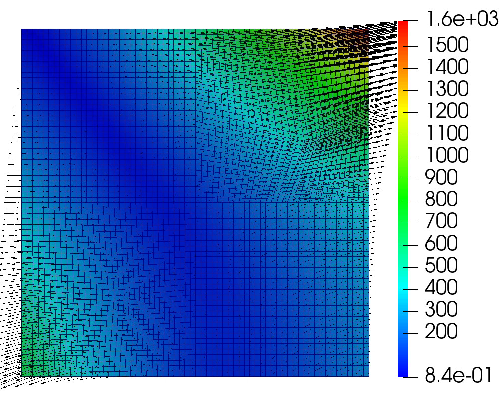
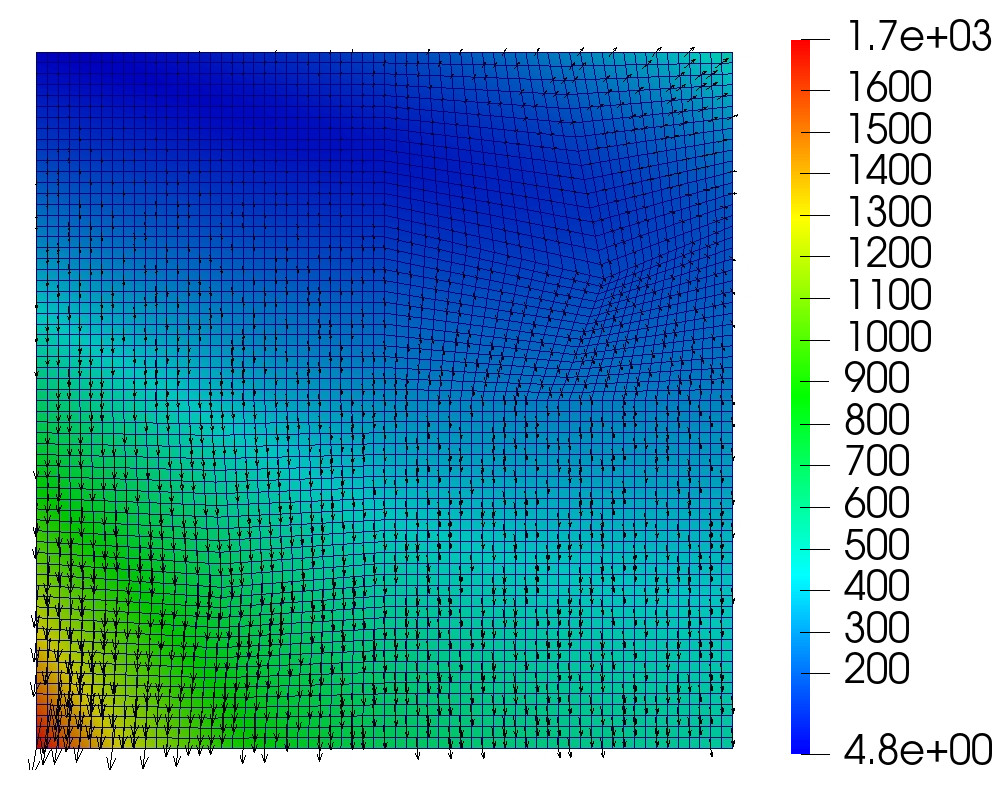
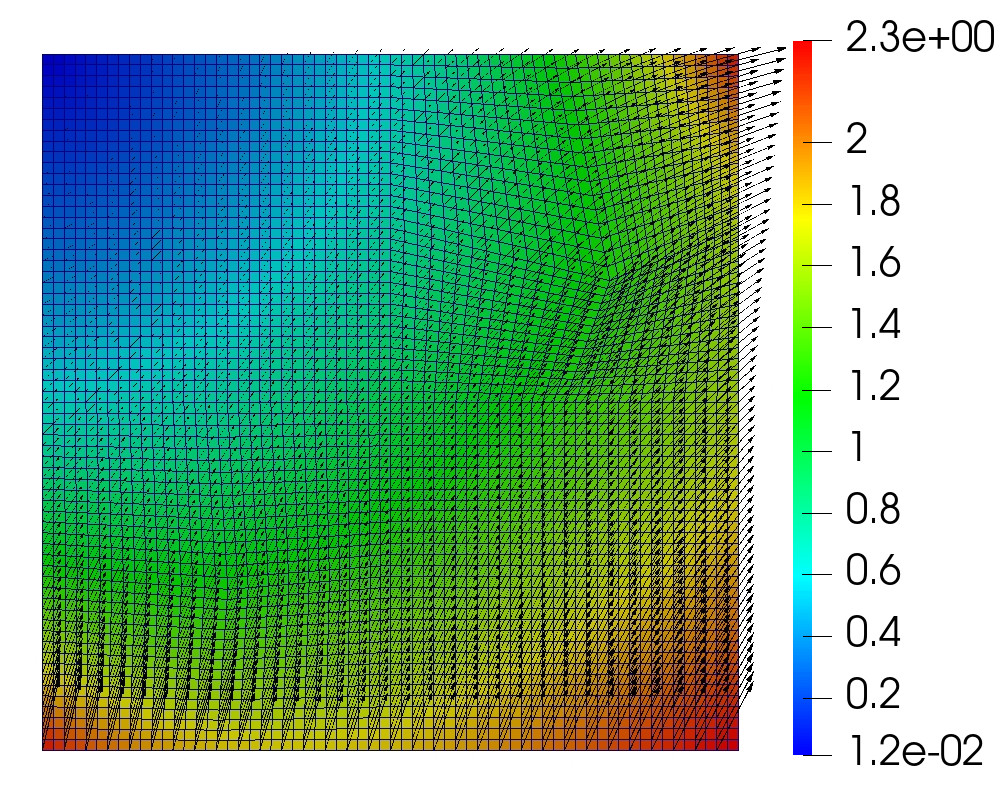
The global mesh is divided into square subdomains. We run a sequence of refinements from to . The initial grids in the bottom left and top right subdomains are perturbed randomly, resulting in general quadrilateral elements. The computed solution for the monolithic scheme with and on the final time step is given in Figure 5.1.
To study and compare the convergence and stability of the three methods, we run tests with time steps . The results with are presented in Tables 2–4. We report the average number of iterations over 100 time steps. The numerical errors are relative to the corresponding norms of the exact solution. We use standard Bochner space notation to denote the space-time norms. Convergence results for the case with and are given in Table 5.
The main observation is that all three methods exhibit growth in the number of interface iterations at the rate of . This is consistent with the theoretical bounds on the spectrum of the interface operator, cf. the discussion at the beginning of Section 5. This behavior is robust with respect to both and . We further note that in both split schemes, the Darcy interface solver requires fewer number of iterations than the elasticity solver. We attribute this to the fact that the Darcy formulation involves a contribution to the diagonal from the time derivative term, resulting in a smaller condition number of the interface operator.
Another important conclusion from the tables is that two split schemes are stable uniformly in and , in accordance with Theorem 4.1 and Theorem 4.2.
In terms of accuracy, all three methods yield convergence for all variables in their natural norms, which is optimal convergence for the approximation of the Biot system with the chosen finite element spaces, cf. [39, 7]. In some cases, especially for larger , we observe reduction in the convergence rate for certain variables due to the effect of the time discretization and/or splitting errors, most notably for the Darcy velocity in the fixed stress scheme. The accuracy of the three methods is comparable for smaller .
In terms of efficiency, in most cases the total number of flow and elasticity CG iterations in the split schemes is comparable to the number of GMRES iterations in the monolithic scheme. However, the split schemes have a clear advantage, due to the more efficient CG interface solver compared to GMRES for the monolithic scheme, as well as the less costly subdomain problems - single-physics solves versus the coupled Biot solves in the monolithic scheme.

| #GMRES | ||||||||||
|---|---|---|---|---|---|---|---|---|---|---|
| 24 | rate | 2.13e+00 | rate | 7.05e-02 | rate | 6.95e-01 | rate | 6.88e-01 | rate | |
| 33 | -0.46 | 1.13e+00 | 0.92 | 3.56e-02 | 0.98 | 3.57e-01 | 0.96 | 3.48e-01 | 0.98 | |
| 44 | -0.42 | 4.84e-01 | 1.22 | 1.79e-02 | 1.00 | 1.79e-01 | 0.99 | 1.75e-01 | 1.00 | |
| 62 | -0.49 | 2.01e-01 | 1.27 | 8.94e-03 | 1.00 | 8.99e-02 | 1.00 | 8.74e-02 | 1.00 | |
| 87 | -0.49 | 9.15e-02 | 1.14 | 4.47e-03 | 1.00 | 4.50e-02 | 1.00 | 4.37e-02 | 1.00 | |
| #CGElast | #CGDarcy | |||||||||||
|---|---|---|---|---|---|---|---|---|---|---|---|---|
| 19 | rate | 10 | rate | 2.00e+00 | rate | 7.07e-02 | rate | 7.01e-01 | rate | 6.88e-01 | rate | |
| 23 | -0.28 | 10 | 0.00 | 1.11e+00 | 0.85 | 3.57e-02 | 0.99 | 3.59e-01 | 0.96 | 3.48e-01 | 0.98 | |
| 34 | -0.56 | 11 | -0.14 | 4.89e-01 | 1.18 | 1.79e-02 | 1.00 | 1.81e-01 | 0.99 | 1.75e-01 | 1.00 | |
| 47 | -0.47 | 15 | -0.45 | 2.06e-01 | 1.25 | 8.94e-03 | 1.00 | 9.06e-02 | 1.00 | 8.74e-02 | 1.00 | |
| 65 | -0.47 | 20 | -0.42 | 9.29e-02 | 1.15 | 4.47e-03 | 1.00 | 4.53e-02 | 1.00 | 4.37e-02 | 1.00 | |
| #CGElast | #CGDarcy | |||||||||||
|---|---|---|---|---|---|---|---|---|---|---|---|---|
| 19 | rate | 10 | rate | 1.93e+00 | rate | 7.06e-02 | rate | 7.01e-01 | rate | 6.88e-01 | rate | |
| 23 | -0.28 | 10 | 0.00 | 1.05e+00 | 0.88 | 3.56e-02 | 0.99 | 3.59e-01 | 0.96 | 3.48e-01 | 0.98 | |
| 34 | -0.56 | 11 | -0.14 | 4.46e-01 | 1.23 | 1.79e-02 | 1.00 | 1.81e-01 | 0.99 | 1.75e-01 | 1.00 | |
| 47 | -0.47 | 15 | -0.45 | 2.63e-01 | 0.76 | 8.95e-03 | 1.00 | 9.06e-02 | 1.00 | 8.74e-02 | 1.00 | |
| 65 | -0.47 | 20 | -0.42 | 2.17e-01 | 0.28 | 4.49e-03 | 0.99 | 4.53e-02 | 1.00 | 4.37e-02 | 1.00 | |
| #GMRES | ||||||||||
|---|---|---|---|---|---|---|---|---|---|---|
| 18 | rate | 1.58e+00 | rate | 6.98e-02 | rate | 6.97e-01 | rate | 6.88e-01 | rate | |
| 23 | -0.35 | 7.47e-01 | 1.08 | 3.55e-02 | 0.97 | 3.58e-01 | 0.96 | 3.48e-01 | 0.98 | |
| 32 | -0.48 | 3.58e-01 | 1.06 | 1.79e-02 | 0.99 | 1.80e-01 | 0.99 | 1.75e-01 | 0.99 | |
| 44 | -0.46 | 1.77e-01 | 1.02 | 8.97e-03 | 0.99 | 9.02e-02 | 1.00 | 8.88e-02 | 0.98 | |
| 63 | -0.52 | 8.98e-02 | 0.98 | 4.54e-03 | 0.98 | 4.53e-02 | 1.00 | 4.66e-02 | 0.93 | |
| #CGElast | #CGDarcy | |||||||||||
|---|---|---|---|---|---|---|---|---|---|---|---|---|
| 19 | rate | 10 | rate | 1.57e+00 | rate | 6.98e-02 | rate | 7.01e-01 | rate | 6.88e-01 | rate | |
| 23 | -0.28 | 12 | -0.26 | 7.46e-01 | 1.07 | 3.55e-02 | 0.97 | 3.59e-01 | 0.96 | 3.48e-01 | 0.98 | |
| 34 | -0.56 | 16 | -0.42 | 3.58e-01 | 1.06 | 1.79e-02 | 0.99 | 1.81e-01 | 0.99 | 1.75e-01 | 1.00 | |
| 47 | -0.47 | 23 | -0.52 | 1.77e-01 | 1.02 | 8.97e-03 | 0.99 | 9.06e-02 | 1.00 | 8.74e-02 | 1.00 | |
| 65 | -0.47 | 32 | -0.48 | 8.96e-02 | 0.98 | 4.53e-03 | 0.98 | 4.53e-02 | 1.00 | 4.37e-02 | 1.00 | |
| #CGElast | #CGDarcy | |||||||||||
|---|---|---|---|---|---|---|---|---|---|---|---|---|
| 19 | rate | 10 | rate | 1.48e+00 | rate | 6.97e-02 | rate | 7.01e-01 | rate | 6.88e-01 | rate | |
| 23 | -0.28 | 12 | -0.26 | 7.64e-01 | 0.96 | 3.56e-02 | 0.97 | 3.59e-01 | 0.96 | 3.48e-01 | 0.98 | |
| 34 | -0.56 | 16 | -0.42 | 4.88e-01 | 0.65 | 1.81e-02 | 0.98 | 1.81e-01 | 0.99 | 1.75e-01 | 1.00 | |
| 47 | -0.47 | 23 | -0.52 | 3.80e-01 | 0.36 | 9.37e-03 | 0.95 | 9.06e-02 | 1.00 | 8.74e-02 | 1.00 | |
| 65 | -0.47 | 32 | -0.48 | 3.44e-01 | 0.14 | 5.26e-03 | 0.83 | 4.53e-02 | 1.00 | 4.37e-02 | 1.00 | |
| #GMRES | ||||||||||
|---|---|---|---|---|---|---|---|---|---|---|
| 40 | rate | 1.38e+00 | rate | 6.99e-02 | rate | 7.04e-01 | rate | 7.17e-01 | rate | |
| 59 | -0.56 | 7.20e-01 | 0.94 | 3.63e-02 | 0.94 | 3.65e-01 | 0.95 | 4.26e-01 | 0.75 | |
| 88 | -0.58 | 3.97e-01 | 0.86 | 1.94e-02 | 0.90 | 1.92e-01 | 0.93 | 3.09e-01 | 0.46 | |
| 128 | -0.54 | 2.57e-01 | 0.63 | 1.17e-02 | 0.72 | 1.09e-01 | 0.81 | 2.72e-01 | 0.19 | |
| 180 | -0.49 | 2.08e-01 | 0.31 | 8.84e-03 | 0.41 | 7.40e-02 | 0.56 | 2.62e-01 | 0.06 | |
| #CGElast | #CGDarcy | |||||||||||
|---|---|---|---|---|---|---|---|---|---|---|---|---|
| 19 | rate | 11 | rate | 1.38e+00 | rate | 6.99e-02 | rate | 7.01e-01 | rate | 6.88e-01 | rate | |
| 23 | -0.28 | 14 | -0.35 | 7.17e-01 | 0.94 | 3.62e-02 | 0.95 | 3.59e-01 | 0.96 | 3.48e-01 | 0.98 | |
| 34 | -0.56 | 20 | -0.51 | 3.92e-01 | 0.87 | 1.92e-02 | 0.91 | 1.81e-01 | 0.99 | 1.75e-01 | 1.00 | |
| 47 | -0.47 | 28 | -0.49 | 2.50e-01 | 0.65 | 1.15e-02 | 0.75 | 9.07e-02 | 1.00 | 8.74e-02 | 1.00 | |
| 65 | -0.47 | 38 | -0.44 | 1.99e-01 | 0.33 | 8.48e-03 | 0.44 | 4.56e-02 | 0.99 | 4.37e-02 | 1.00 | |
| #CGElast | #CGDarcy | |||||||||||
|---|---|---|---|---|---|---|---|---|---|---|---|---|
| 19 | rate | 11 | rate | 1.42e+00 | rate | 7.00e-02 | rate | 7.00e-01 | rate | 6.88e-01 | rate | |
| 23 | -0.28 | 14 | -0.35 | 8.38e-01 | 0.76 | 3.63e-02 | 0.95 | 3.59e-01 | 0.96 | 3.48e-01 | 0.98 | |
| 34 | -0.56 | 20 | -0.51 | 5.83e-01 | 0.52 | 1.93e-02 | 0.91 | 1.81e-01 | 0.99 | 1.75e-01 | 1.00 | |
| 47 | -0.47 | 28 | -0.49 | 4.87e-01 | 0.26 | 1.15e-02 | 0.74 | 9.06e-02 | 1.00 | 8.74e-02 | 1.00 | |
| 65 | -0.47 | 38 | -0.44 | 4.56e-01 | 0.09 | 8.53e-03 | 0.44 | 4.53e-02 | 1.00 | 4.37e-02 | 1.00 | |
| #GMRES | ||||||||||
|---|---|---|---|---|---|---|---|---|---|---|
| 21 | rate | 1.86e+00 | rate | 7.12e-02 | rate | 6.97e-01 | rate | 6.88e-01 | rate | |
| 28 | -0.42 | 7.87e-01 | 1.24 | 3.57e-02 | 1.00 | 3.58e-01 | 0.96 | 3.48e-01 | 0.98 | |
| 38 | -0.44 | 3.63e-01 | 1.12 | 1.79e-02 | 1.00 | 1.80e-01 | 0.99 | 1.75e-01 | 0.99 | |
| 53 | -0.48 | 1.77e-01 | 1.04 | 8.94e-03 | 1.00 | 9.02e-02 | 1.00 | 8.88e-02 | 0.98 | |
| 73 | -0.46 | 8.78e-02 | 1.01 | 4.47e-03 | 1.00 | 4.53e-02 | 1.00 | 4.66e-02 | 0.93 | |
| #CGElast | #CGDarcy | |||||||||||
|---|---|---|---|---|---|---|---|---|---|---|---|---|
| 19 | rate | 11 | rate | 1.90e+00 | rate | 7.16e-02 | rate | 7.01e-01 | rate | 6.88e-01 | rate | |
| 23 | -0.28 | 15 | -0.45 | 7.91e-01 | 1.26 | 3.58e-02 | 1.00 | 3.59e-01 | 0.96 | 3.48e-01 | 0.98 | |
| 34 | -0.56 | 20 | -0.42 | 3.64e-01 | 1.12 | 1.79e-02 | 1.00 | 1.81e-01 | 0.99 | 1.75e-01 | 1.00 | |
| 47 | -0.47 | 28 | -0.49 | 1.78e-01 | 1.03 | 8.98e-03 | 1.00 | 9.06e-02 | 1.00 | 8.74e-02 | 1.00 | |
| 65 | -0.47 | 41 | -0.55 | 9.01e-02 | 0.98 | 4.55e-03 | 0.98 | 4.53e-02 | 1.00 | 4.37e-02 | 1.00 | |
| #CGElast | #CGDarcy | |||||||||||
|---|---|---|---|---|---|---|---|---|---|---|---|---|
| 19 | rate | 11 | rate | 1.88e+00 | rate | 7.16e-02 | rate | 7.01e-01 | rate | 6.88e-01 | rate | |
| 23 | -0.28 | 15 | -0.45 | 8.84e-01 | 1.09 | 3.72e-02 | 0.94 | 3.59e-01 | 0.96 | 3.48e-01 | 0.98 | |
| 34 | -0.56 | 20 | -0.42 | 6.43e-01 | 0.46 | 2.08e-02 | 0.84 | 1.81e-01 | 0.99 | 1.75e-01 | 1.00 | |
| 47 | -0.47 | 28 | -0.49 | 5.60e-01 | 0.20 | 1.36e-02 | 0.61 | 9.06e-02 | 1.00 | 8.74e-02 | 1.00 | |
| 65 | -0.47 | 41 | -0.55 | 5.36e-01 | 0.06 | 1.10e-02 | 0.31 | 4.53e-02 | 1.00 | 4.37e-02 | 1.00 | |
5.2 Example 2: dependence on number of subdomains
The objective of this example is to study how the number of GMRES and CG iterations required for the different schemes depend on the number (and diameter) of subdomains used in the domain decomposition. For this example, we use the same test case as in Example 1. We solve the system using 4 , 16 , and 64 square subdomains of identical size. The physical parameters are as in Example 1, with , , and . The average number and growth rate of iterations in the three methods are reported in Tables 6–8, where denotes the subdomain diameter. We note that the number of iterations for the drained split and fixed stress schemes are identical, so we give one table for both methods. For a fixed , the growth rate with respect to is averaged over all mesh refinements. For a fixed mesh size , the growth rate with respect to is averaged over the different domain decompositions. For all three methods, we observe that for a fixed number of subdomains, the growth rate in the number of iterations with respect to mesh refinement is approximately , being slightly better for the Darcy solver in the split schemes. As this is the same as the growth rate in Example 1, the conclusion from Example 1 that the growth rate is consistent with the theory extends to domain decompositions with varying number of subdomains, see also the discussion at the beginning of Section 5. We further observe that for a fixed mesh size, the growth rate in number of iterations with respect to subdomain diameter is approximately , again being somewhat better for the Darcy solves. This is consistent with theoretical results bounding the spectral ratio of the unpreconditioned interface operator as [57]. The dependence on can be eliminated with the use of a coarse solve preconditioner [58, 57].
| Rate | ||||
|---|---|---|---|---|
| 33 | 53 | 76 | ||
| 45 | 68 | 97 | ||
| 63 | 93 | 126 | ||
| 88 | 125 | 164 | ||
| Rate |
| Rate | ||||
|---|---|---|---|---|
| 23 | 40 | 60 | ||
| 34 | 51 | 73 | ||
| 47 | 68 | 95 | ||
| 65 | 95 | 124 | ||
| Rate |
| Rate | ||||
|---|---|---|---|---|
| 10 | 11 | 14 | ||
| 11 | 12 | 14 | ||
| 15 | 16 | 18 | ||
| 20 | 23 | 24 | ||
| Rate |
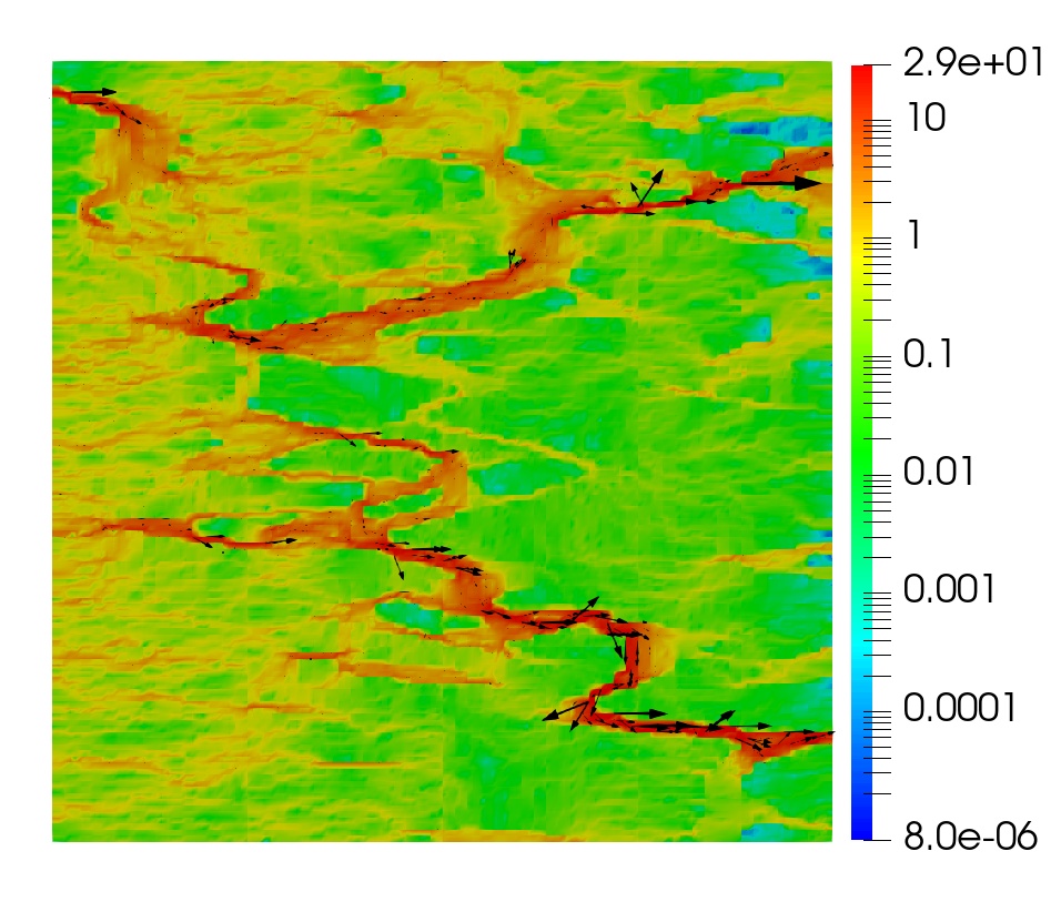
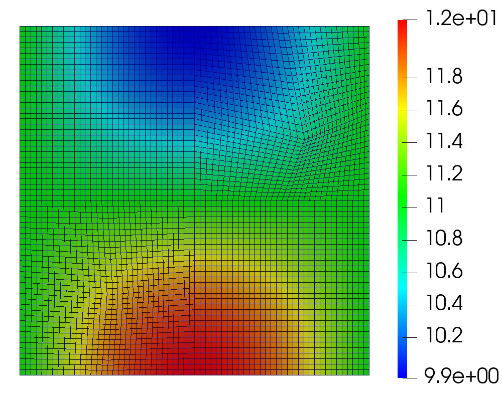
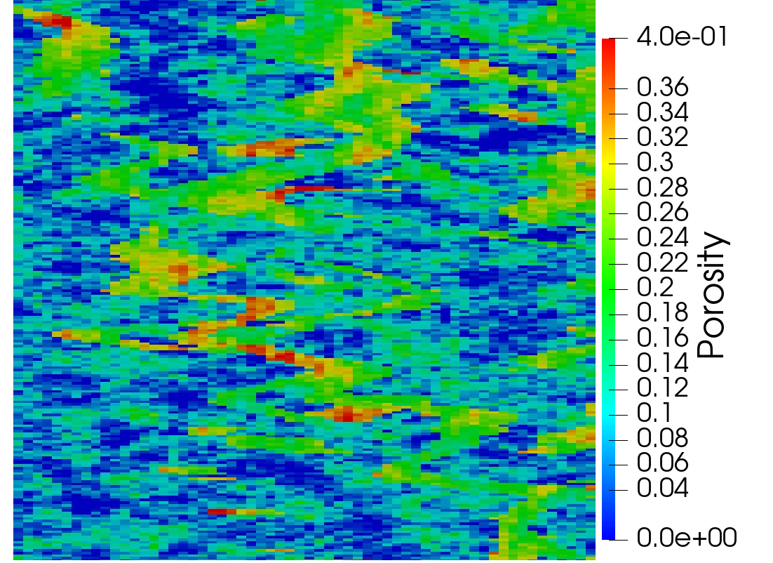
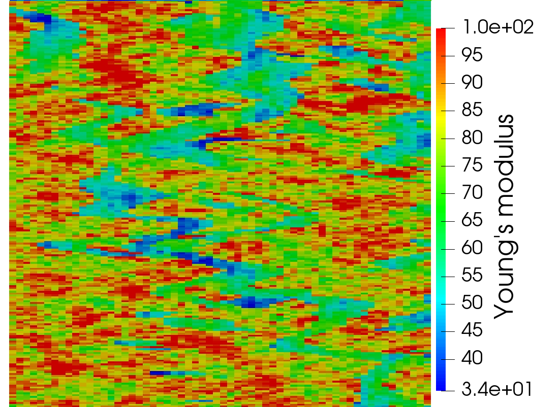
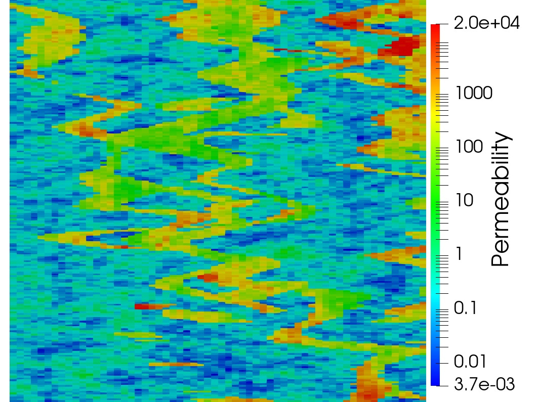
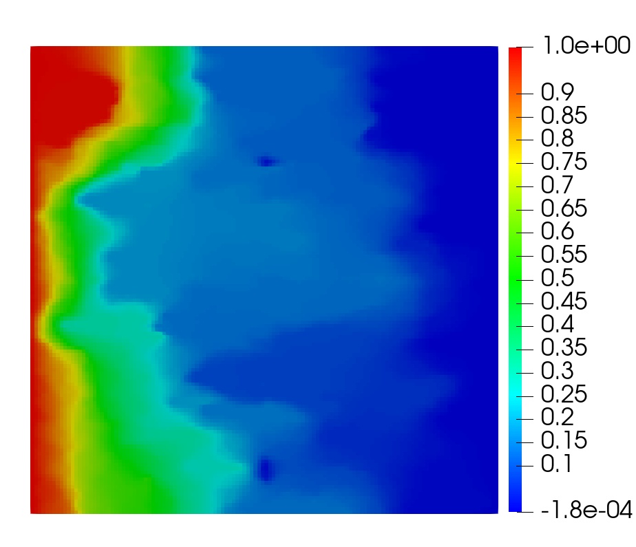
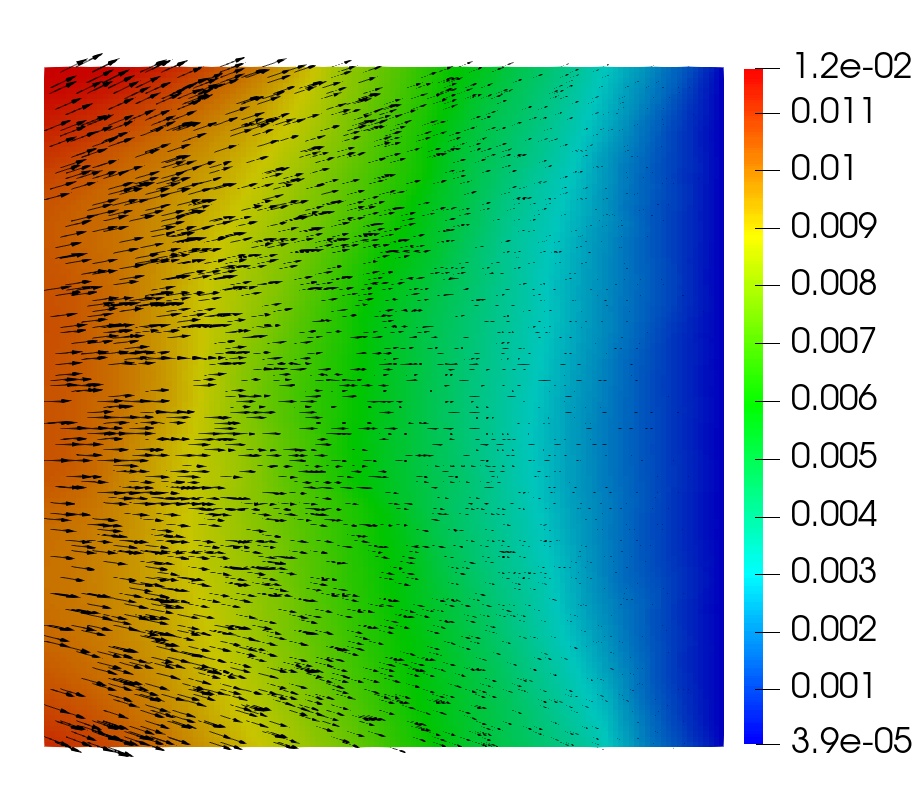
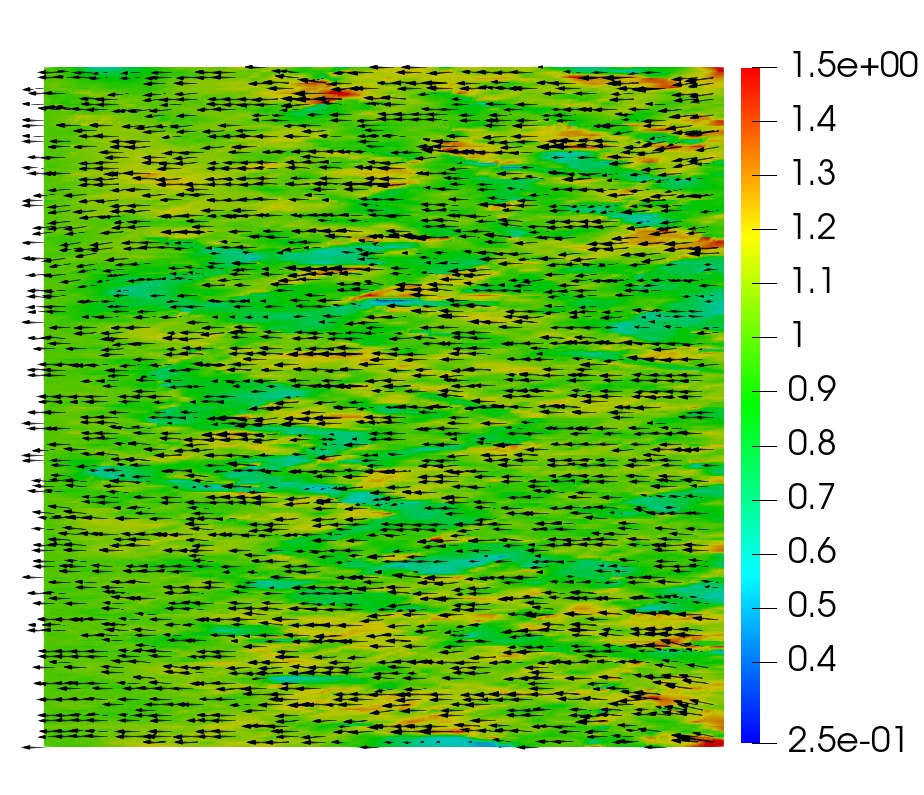
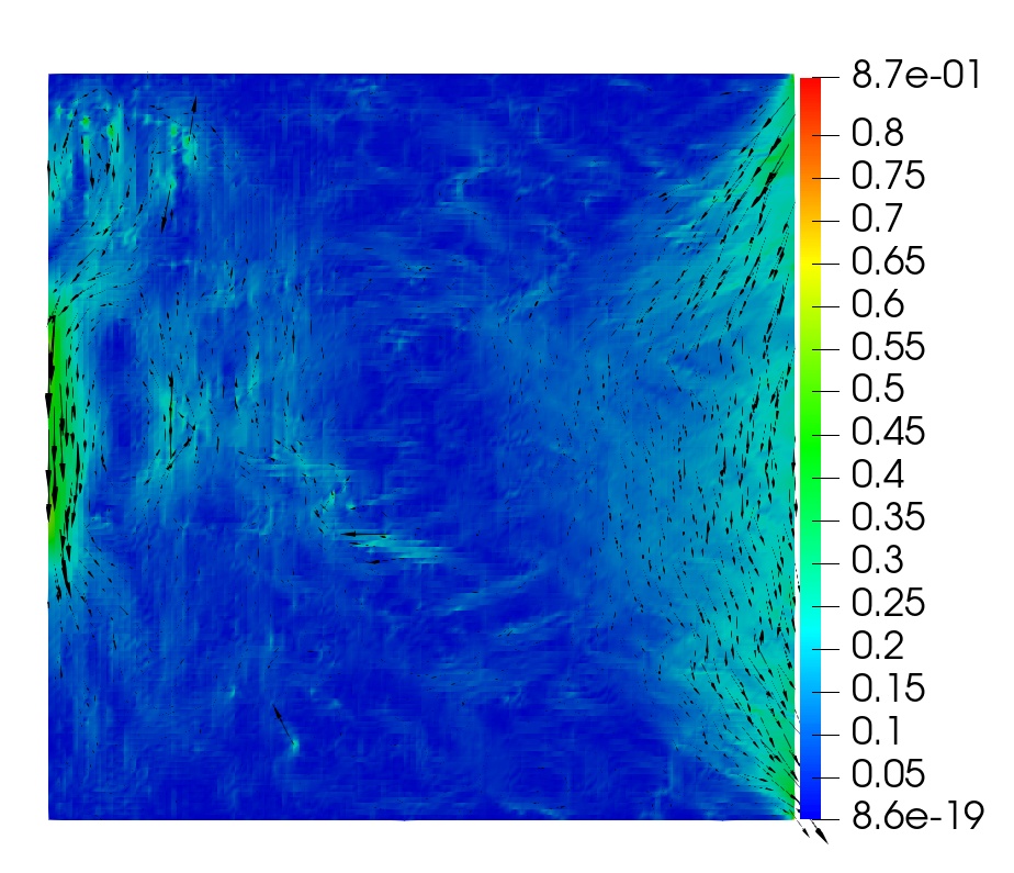
5.3 Example 3: heterogeneous benchmark
This example illustrates the performance of the methods for highly heterogeneous media. We use porosity and permeability fields from the Society of Petroleum Engineers 10th Comparative Solution Project (SPE10)111https://www.spe.org/web/csp/datasets/set02.htm. The computational domain is , which is partitioned into a square grid. We decompose the domain into square subdomains. From the porosity field data, the Young’s modulus is obtained using the relation where , refers to the porosity at which the Young’s modulus vanishes, see [38] for details. The porosity, Young’s modulus and permeability fields are given in Figure 5.2. The parameters and boundary conditions are given in Table 9. The source terms are taken to be zero. These conditions describe flow from left to right, driven by a pressure gradient. Since in this example analytical solution is not available, we need to prescribe suitable initial data. The initial condition for the pressure is taken to be , which is compatible with the prescribed boundary conditions. We then follow the procedure described in Remark 3.1 to obtain discrete initial data. In particular, we set to be the -projection of onto and solve a mixed elasticity domain decomposition problem at to obtain . We note that this solve also gives , , and . In the case of the monolithic scheme where the time-differentiated elasticity equation (3.8) is solved, the computed initial data is used to recover , , and using (3.16). The computed solution using the monolithic domain decomposition scheme is given in Figure 5.3. The solutions from the two split methods look similar.
| Parameter | Value |
|---|---|
| Mass storativity | |
| Biot-Willis constant | |
| Time step | |
| Total time |
| Boundary | ||||
|---|---|---|---|---|
| Left | - | - | ||
| Bottom | - | - | ||
| Right | - | |||
| Top | - | - |
In Table 10, we compare the average number of interface iterations per time step in the three methods. All three methods converge for this highly heterogeneous problem with realistic physical parameters. While the three methods provide similar solutions and the number of interface iterations is comparable, the split methods are more efficient than the monolithic method, due the less expensive CG iterations and single-physics subdomain solves. We further note that in the split methods the Darcy interface solve is more expensive than the elasticity one, which is likely due to the fact that the permeability varies over seven orders of magnitude, affecting the condition number of the interface operator.
| Monolithic | Drained Split | Fixed Stress | |||
| #GMRES | #CGElast | #CGDarcy | #CGElast | #CGDarcy | |
6 Conclusions
We presented three non-overlapping domain decomposition methods for the Biot system of poroelasticity in a five-field fully mixed formulation. The monolithic method involves solving an interface problem for a composite displacement-pressure Lagrange multiplier, which requires coupled Biot subdomain solves at each iteration. The two split methods are based on the drained split and fixed stress splittings. They involve two separate elasticity and Darcy interface iterations requiring single-physics subdomain solves. We analyze the spectrum of the monolithic interface operator and show unconditional stability for the split methods. A series of numerical experiments illustrate the efficiency, accuracy, and robustness of the three methods. Our main conclusion is that while two approaches are comparable in terms of accuracy and number of interface iterations, the split methods are more computationally efficient than the monolithic method due to the less expensive CG iterations compared to GMRES and simpler single-physics subdomain solves compared to coupled Biot solves in the monolithic method.
References
- [1] E. Ahmed, J. M. Nordbotten, and F. A. Radu. Adaptive asynchronous time-stepping, stopping criteria, and a posteriori error estimates for fixed-stress iterative schemes for coupled poromechanics problems. J. Comput. Appl. Math., 364:112312, 25, 2020.
- [2] E. Ahmed, F. A. Radu, and J. M. Nordbotten. Adaptive poromechanics computations based on a posteriori error estimates for fully mixed formulations of Biot’s consolidation model. Comput. Methods Appl. Mech. Engrg., 347:264–294, 2019.
- [3] T. Almani, K. Kumar, A. Dogru, G. Singh, and M. F. Wheeler. Convergence analysis of multirate fixed-stress split iterative schemes for coupling flow with geomechanics. Comput. Methods Appl. Mech. Engrg., 311:180–207, 2016.
- [4] G. Alzetta, D. Arndt, W. Bangerth, V. Boddu, B. Brands, D. Davydov, R. Gassmoeller, T. Heister, L. Heltai, K. Kormann, M. Kronbichler, M. Maier, J.-P. Pelteret, B. Turcksin, and D. Wells. The deal.II library, version 9.0. Journal of Numerical Mathematics, 26(4):173–183, 2018.
- [5] M. Amara and J. M. Thomas. Equilibrium finite elements for the linear elastic problem. Numer. Math., 33(4):367–383, 1979.
- [6] I. Ambartsumyan, E. Khattatov, J. M. Nordbotten, and I. Yotov. A multipoint stress mixed finite element method for elasticity on quadrilateral grids. Numer. Methods Partial Differential Equations, https://doi.org/10.1002/num.22624, 2020.
- [7] I. Ambartsumyan, E. Khattatov, and I. Yotov. A coupled multipoint stress - multipoint flux mixed finite element method for the Biot system of poroelasticity. Comput. Methods Appl. Mech. Engrg., 372:113407, 2020.
- [8] T. Arbogast, L. C. Cowsar, M. F. Wheeler, and I. Yotov. Mixed finite element methods on nonmatching multiblock grids. SIAM J. Numer. Anal., 37(4):1295–1315, 2000.
- [9] D. N. Arnold, G. Awanou, and W. Qiu. Mixed finite elements for elasticity on quadrilateral meshes. Adv. Comput. Math., 41(3):553–572, 2015.
- [10] D. N. Arnold, R. S. Falk, and R. Winther. Mixed finite element methods for linear elasticity with weakly imposed symmetry. Math. Comp., 76(260):1699–1723, 2007.
- [11] G. Awanou. Rectangular mixed elements for elasticity with weakly imposed symmetry condition. Adv. Comput. Math., 38(2):351–367, 2013.
- [12] W. Bangerth, R. Hartmann, and G. Kanschat. deal.II – a general purpose object oriented finite element library. ACM Trans. Math. Softw., 33(4):24/1–24/27, 2007.
- [13] M. Bause, F. Radu, and U. Kocher. Space-time finite element approximation of the Biot poroelasticity system with iterative coupling. Comput. Methods Appl. Mech. Engrg., 320:745–768, 2017.
- [14] M. A. Biot. General theory of three-dimensional consolidation. J. Appl. Phys., 12(2):155–164, 1941.
- [15] D. Boffi, F. Brezzi, L. F. Demkowicz, R. G. Durán, R. S. Falk, and M. Fortin. Mixed finite elements, compatibility conditions, and applications, volume 1939 of Lecture Notes in Mathematics. Springer-Verlag, Berlin; Fondazione C.I.M.E., Florence, 2008.
- [16] D. Boffi, F. Brezzi, and M. Fortin. Reduced symmetry elements in linear elasticity. Commun. Pure Appl. Anal., 8(1):95–121, 2009.
- [17] M. Borregales, K. Kumar, F. A. Radu, C. Rodrigo, and F. J. Gaspar. A partially parallel-in-time fixed-stress splitting method for Biot’s consolidation model. Comput. Math. Appl., 77(6):1466–1478, 2019.
- [18] J. W. Both, K. Kumar, J. M. Nordbotten, and F. A. Radu. Anderson accelerated fixed-stress splitting schemes for consolidation of unsaturated porous media. Comput. Math. Appl., 77(6):1479–1502, 2019.
- [19] F. Brezzi and M. Fortin. Mixed and hybrid finite element methods, volume 15 of Springer Series in Computational Mathematics. Springer-Verlag, New York, 1991.
- [20] M. Bukac, W. Layton, M. Moraiti, H. Tran, and C. Trenchea. Analysis of partitioned methods for the Biot system. Numer. Methods Partial Differential Equations, 31(6):1769–1813, 2015.
- [21] B. Cockburn, J. Gopalakrishnan, and J. Guzmán. A new elasticity element made for enforcing weak stress symmetry. Math. Comp., 79(271):1331–1349, 2010.
- [22] L. C. Cowsar, J. Mandel, and M. F. Wheeler. Balancing domain decomposition for mixed finite elements. Math. Comp., 64(211):989–1015, 1995.
- [23] M. Dauge. Elliptic boundary value problems on corner domains, volume 1341 of Lecture Notes in Mathematics. Springer-Verlag, Berlin, 1988.
- [24] M. Farhloul and M. Fortin. Dual hybrid methods for the elasticity and the Stokes problems: a unified approach. Numer. Math., 76(4):419–440, 1997.
- [25] H. Florez. About revisiting domain decomposition methods for poroelasticity. Mathematics, 6(10):187, 2018.
- [26] H. Florez and M. Wheeler. A mortar method based on NURBS for curved interfaces. Comput. Methods Appl. Mech. Engrg., 310:535–566, 2016.
- [27] F. J. Gaspar, F. J. Lisbona, and P. N. Vabishchevich. A finite difference analysis of Biot’s consolidation model. Appl. Numer. Math., 44(4):487–506, 2003.
- [28] V. Girault, G. Pencheva, M. F. Wheeler, and T. Wildey. Domain decomposition for poroelasticity and elasticity with DG jumps and mortars. Math. Mod. Meth. Appl. S., 21(01):169–213, 2011.
- [29] R. Glowinski and M. F. Wheeler. Domain decomposition and mixed finite element methods for elliptic problems. In First international symposium on domain decomposition methods for partial differential equations, pages 144–172, 1988.
- [30] J. Gopalakrishnan and J. Guzmán. A second elasticity element using the matrix bubble. IMA J. Numer. Anal., 32(1):352–372, 2012.
- [31] P. Gosselet, V. Chiaruttini, C. Rey, and F. Feyel. A monolithic strategy based on an hybrid domain decomposition method for multiphysic problems. Application to poroelasticity. Revue Europeenne des Elements Finis, 13:523–534, 2012.
- [32] X. Hu, C. Rodrigo, F. J. Gaspar, and L. T. Zikatanov. A nonconforming finite element method for the Biot’s consolidation model in poroelasticity. J. Comput. Appl. Math., 310:143–154, 2017.
- [33] I. C. F. Ipsen. Expressions and bounds for the GMRES residual. BIT Numerical Mathematics, 40(3):524–535, 2000.
- [34] C. T. Kelley. Iterative methods for linear and nonlinear equations, volume 16 of Frontiers in Applied Mathematics. Society for Industrial and Applied Mathematics, Philadelphia, 1995.
- [35] E. Khattatov and I. Yotov. Domain decomposition and multiscale mortar mixed finite element methods for linear elasticity with weak stress symmetry. ESAIM Math. Model. Numer. Anal., 53(6):2081–2108, 2019.
- [36] J. Kim, H. Tchelepi, and R. Juanes. Stability and convergence of sequential methods for coupled flow and geomechanics: Drained and undrained splits. Comput. Methods Appl. Mech. Engrg., 200:2094–2116, 2011.
- [37] J. Kim, H. Tchelepi, and R. Juanes. Stability and convergence of sequential methods for coupled flow and geomechanics: Fixed-stress and fixed-strain splits. Comput. Methods Appl. Mech. Engrg., 200:1591–1606, 2011.
- [38] J. Kovacik. Correlation between Young’s modulus and porosity in porous materials. J. Mater. Sci. Lett., 18(13):1007–1010, 1999.
- [39] J. J. Lee. Robust error analysis of coupled mixed methods for Biot’s consolidation model. J. Sci. Comput., 69(2):610–632, 2016.
- [40] J. J. Lee. Towards a unified analysis of mixed methods for elasticity with weakly symmetric stress. Adv. Comput. Math., 42(2):361–376, 2016.
- [41] J. J. Lee. Robust three-field finite element methods for Biot’s consolidation model in poroelasticity. BIT, 58(2):347–372, 2018.
- [42] J. J. Lee, K.-A. Mardal, and R. Winther. Parameter-robust discretization and preconditioning of Biot’s consolidation model. SIAM J. Sci. Comput., 39(1):A1–A24, 2017.
- [43] T. P. Mathew. Domain decomposition and iterative refinement methods for mixed finite element discretizations of elliptic problems. PhD thesis, Courant Institute of Mathematical Sciences, New York University, 1989. Tech. Rep. 463.
- [44] A. Mikelić and M. F. Wheeler. Convergence of iterative coupling for coupled flow and geomechanics. Comput. Geosci., 17(3):455–461, 2013.
- [45] M. A. Murad and A. F. D. Loula. Improved accuracy in finite element analysis of Biot’s consolidation problem. Comput. Methods Appl. Mech. Engrg., 95(3):359–382, 1992.
- [46] J. M. Nordbotten. Stable cell-centered finite volume discretization for Biot equations. SIAM J. Numer. Anal., 54(2):942–968, 2016.
- [47] R. Oyarzúa and R. Ruiz-Baier. Locking-free finite element methods for poroelasticity. SIAM J. Numer. Anal., 54(5):2951–2973, 2016.
- [48] P. J. Phillips and M. F. Wheeler. A coupling of mixed and continuous Galerkin finite element methods for poroelasticity. I. The continuous in time case. Comput. Geosci., 11(2):131–144, 2007.
- [49] P. J. Phillips and M. F. Wheeler. A coupling of mixed and discontinuous Galerkin finite-element methods for poroelasticity. Comput. Geosci., 12(4):417–435, 2008.
- [50] A. Quarteroni and A. Valli. Domain Decomposition Methods for Partial Differential equations. Clarendon Press, Oxford, 1999.
- [51] C. Rodrigo, F. J. Gaspar, X. Hu, and L. T. Zikatanov. Stability and monotonicity for some discretizations of the Biot’s consolidation model. Comput. Methods Appl. Mech. Engrg., 298:183–204, 2016.
- [52] C. Rodrigo, X. Hu, P. Ohm, J. H. Adler, F. J. Gaspar, and L. T. Zikatanov. New stabilized discretizations for poroelasticity and the Stokes’ equations. Comput. Methods Appl. Mech. Engrg., 341:467–484, 2018.
- [53] R. E. Showalter. Diffusion in poro-elastic media. J. Math. Anal. Appl., 251(1):310 – 340, 2000.
- [54] G. Starke. Field-of-values analysis of preconditioned iterative methods for nonsymmetric elliptic problems. Numer. Math., 78(1):103–117, 1997.
- [55] R. Stenberg. A family of mixed finite elements for the elasticity problem. Numer. Math., 53(5):513–538, 1988.
- [56] E. Storvik, J. W. Both, K. Kumar, J. M. Nordbotten, and F. A. Radu. On the optimization of the fixed-stress splitting for Biot’s equations. Int. J. Numer. Methods. Eng., 120(2):179–194, 2019.
- [57] A. Toselli and O. Widlund. Domain decomposition methods—algorithms and theory, volume 34 of Springer Series in Computational Mathematics. Springer-Verlag, Berlin, 2005.
- [58] D. Vassilev, C. Wang, and I. Yotov. Domain decomposition for coupled Stokes and Darcy flows. Comput. Methods. Appl. Mech. Eng., 268:264–283, 2014.
- [59] M. F. Wheeler, G. Xue, and I. Yotov. Coupling multipoint flux mixed finite element methods with continuous Galerkin methods for poroelasticity. Comput. Geosci., 18(1):57–75, 2014.
- [60] S.-Y. Yi. A coupling of nonconforming and mixed finite element methods for Biot’s consolidation model. Numer. Meth. Partial. Differ. Equ., 29(5):1749–1777, 2013.
- [61] S.-Y. Yi. Convergence analysis of a new mixed finite element method for Biot’s consolidation model. Numer. Meth. Partial. Differ. Equ., 30(4):1189–1210, 2014.
- [62] S.-Y. Yi. A study of two modes of locking in poroelasticity. SIAM J. Numer. Anal., 55(4):1915–1936, 2017.
- [63] S.-Y. Yi and M. Bean. Iteratively coupled solution strategies for a four-field mixed finite element method for poroelasticity. Int. J. Numer. Anal. Meth. Geomech., 2016.