Domain-Driven Solver (DDS) Version 2.0:
a MATLAB-based Software Package for Convex Optimization Problems in Domain-Driven Form
Abstract.
Domain-Driven Solver (DDS) is a MATLAB-based software package for convex optimization problems in Domain-Driven form [19]. The current version of DDS accepts every combination of the following function/set constraints: (1) symmetric cones (LP, SOCP, and SDP); (2) quadratic constraints that are SOCP representable; (3) direct sums of an arbitrary collection of 2-dimensional convex sets defined as the epigraphs of univariate convex functions (including as special cases geometric programming and entropy programming); (4) generalized power cone; (5) epigraphs of matrix norms (including as a special case minimization of nuclear norm over a linear subspace); (6) vector relative entropy; (7) epigraphs of quantum entropy and quantum relative entropy; and (8) constraints involving hyperbolic polynomials. DDS is a practical implementation of the infeasible-start primal-dual algorithm designed and analyzed in [19]. This manuscript contains the users’ guide, as well as theoretical results needed for the implementation of the algorithms. To help the users, we included many examples. We also discussed some implementation details and techniques we used to improve the efficiency and further expansion of the software to cover the emerging classes of convex optimization problems.
Research of the authors was supported in part by Discovery Grants from NSERC and by U.S. Office of Naval Research under award numbers: N00014-12-1-0049, N00014-15-1-2171 and N00014-18-1-2078.
1. Introduction
The code DDS (Domain-Driven Solver) solves convex optimization problems of the form
| (1) |
where is a linear embedding, and are given, and is a closed convex set defined as the closure of the domain of a -self-concordant (s.c.) barrier [27, 26]. In practice, the set is typically formulated as , where is associated with a s.c. barrier , for . Every input constraint for DDS may be thought of as either the convex set it defines or the corresponding s.c. barrier.
The current version of DDS accepts many functions and set constraints as we explain in this article. If a user has a nonlinear convex objective function to minimize, one can introduce a new variable and minimize a linear function subject to the convex set constraint (and other convex constraints in the original optimization problem). As a result, in this article we will talk about representing functions and convex set constraints interchangeably. The algorithm underlying the code also uses the Legendre-Fenchel (LF) conjugate of if it is computationally efficient to evaluate and its first (and hopefully second) derivative. Any new discovery of a s.c. barrier allows DDS to expand the classes of convex optimization problems it can solve as any new s.c. barrier with a computable LF conjugate can be easily added to the code. DDS is a practical implementation of the primal-dual algorithm designed and analyzed in [19], which has the current best iteration complexity bound available for conic formulations. Stopping criteria for DDS and the way DDS suggests the status (“has an approximately optimal solution”, “is infeasible”, “is unbounded”, etc.) is based on the analyses in [20].
Even though there are similarities between DDS and some modeling systems such as CVX [16] (such as the variety input constraints), there are major differences, including:
-
•
DDS is not just a modeling system and it uses its own algorithm. The algorithm used in DDS is an infeasible-start primal-dual path-following algorithm, and is of predictor corrector type [19].
-
•
The modeling systems for convex optimization that rely on SDP solvers have to use approximation for set constraints which are not efficiently representable by spectrahedra (for example epigraph of functions involving or ln functions). However, DDS uses a s.c. barrier specifically well-suited to each set constraint without such approximations. This enables DDS to return proper certificates for all the input problems.
-
•
As far as we know, some set constraints such as hyperbolic ones, are not accepted by other modeling systems. Some other constraints such as epigraphs of matrix norms, and those involving quantum entropy and quantum relative entropy are handled more efficiently than other existing options.
The main part of the article is organized to be more as a users’ guide, and contains the minimum theoretical content required by the users. In Section 2, we explain how to install and use DDS. Sections 3-11 explain how to input different types of set/function constraints into DDS. Section 13 contains several numerical results and tables. Many theoretical foundations needed by DDS are included in the appendices. The LHS matrix of the linear systems of equations determining the predictor and corrector steps have a similar form. In Appendix A, we explain how such linear systems are being solved for DDS. Some of the constraints accepted by DDS are involving matrix functions and many techniques are used in DDS to efficiently evaluate these functions and their derivatives, see Appendices B and C. DDS heavily relies on efficient evaluation of LF conjugates of s.c. barrier functions. For some of the functions, we show in the main text how to efficiently calculate the LF conjugate. For some others, the calculations are shifted to the appendices, for example Appendix D. DDS uses interior-point methods, and gradient and Hessian of the s.c. barriers are building blocks of the underlying linear systems. Explicit formulas for the gradient and Hessian of some s.c. barriers and their LF conjugates are given in Appendix D.2. Appendix F contains a brief comparison of DDS with some popular solvers and modeling systems.
1.1. Installation
The current version of DDS is written in MATLAB. This version is available from the websites:
To use DDS, the user can follow these steps:
-
•
unzip DDS.zip;
-
•
run MATLAB in the directory DDS;
-
•
run the m-file DDS_startup.m.
-
•
(optional) run the prepared small examples DDS_example_1.m and DDS_example_2.m.
The prepared examples contain many set constraints accepted by DDS and running them without error indicates that DDS is ready to use. There is a directory Text_Examples in the DDS package which includes many examples on different classes of convex optimization problems.
2. How to use the DDS code
In this section, we explain the format of the input for many popular classes of optimization problems. In practice, we typically have , where is the domain of a “canonical” s.c. barrier and . For example, for LP, we typically have , where is given as part of the input data, and is a s.c. barrier for . The command in MATLAB that calls DDS is
[x,y,info]=DDS(c,A,b,cons,OPTIONS);
Input Arguments:
cons: A cell array that contains the information about the type of constraints.
c,A,b: Input data for DDS: is the coefficient matrix, is the objective vector, is the RHS vector (i.e., the shift in the definition of the convex domain ).
OPTIONS (optional): An array which contains information about the tolerance and initial points.
Output Arguments:
x: Primal point.
y: Dual point which is a cell array. Each cell contains the dual solution for the constraints in the corresponding cell in A.
info: A structure array containing performance information such as info.time, which returns the CPU time for solving the problem.
Note that in the Domain-Driven setup, the primal problem is the main problem, and the dual problem is implicit for the user. This implicit dual problem is:
| (2) |
where is the support function of , and is defined as
| (3) |
where is the recession cone of . For the convenience of users, there is a built-in function in DDS package to calculate the dual objective value of the returned vector:
z=dual_obj_value(y,b,cons);
For a primal feasible point which satisfies and a dual feasible point , the duality gap is defined in [19] as
| (4) |
It is proved in [19] that the duality gap is well-defined and zero duality gap implies optimality. If DDS returns status “solved” for a problem (info.status=1), it means (x,y) is a pair of approximately feasible primal and dual points, with duality gap close to zero (based on tolerance). If info.status=2, the problem is suspected to be unbounded and the returned x is a point, approximately primal feasible with very small objective value (). If info.status=3, problem is suspected to be infeasible, and the returned y in approximately satisfies with . If info.status=4, problem is suspected to be ill-conditioned.
The user is not required to input any part of the OPTIONS array. The default settings are:
-
•
.
-
•
The initial points and for the infeasible-start algorithm are chosen such that, assuming , the th part of is a canonical point in .
However, if a user chooses to provide OPTIONS as an input, here is how to define the desired parts: OPTIONS.tol may be given as the desired tolerance, otherwise the default is used. OPTIONS.x0 and OPTIONS.z0 may be defined as the initial points as any pair of points and that satisfy . If only OPTIONS.x0 is given, then must satisfy . In other words, OPTIONS.x0 is a point that strictly satisfies all the constraints.
In the following sections, we discuss the format of each input function/set constraint. Table 1 shows the classes of function/set constraints the current version of DDS accepts, plus the abbreviation we use to represent the constraint. From now on, we assume that the objective function is “”, and we show how to add various function/set constraints. Note that A, b, and cons are cell arrays in MATLAB. cons(k,1) represents type of the th block of constraints by using the abbreviations of Table 1. For example, cons(2,1)=’LP’ means that the second block of constraints are linear inequalities. It is advisable to group the constraints of the same type in one block, but not necessary.
| function/set constraint | abbreviation |
|---|---|
| LP | LP |
| SOCP | SOCP |
| Rotated SOCP | SOCPR |
| SDP | SDP |
| Generalized Power Cone | GPC |
| Quadratic Constraints | QC |
| Epigraph of a Matrix Norm | MN |
| Direct sum of 2-dimensional sets | |
| (geometric, entropy, and -norm | TD |
| programming) | |
| Quantum Entropy | QE |
| Quantum Relative Entropy | QRE |
| Relative Entropy | RE |
| Hyperbolic Polynomials | HB |
| Equality Constraints | EQ |
3. LP, SOCP, SDP
3.1. Linear programming (LP) and second-order cone programming (SOCP)
Suppose we want to add LP constraints of the form
| (5) |
where is an -by- matrix, as the th block of constraints. Then, we define
| (12) | |||
| (13) |
Similarly to add SOCP constraints of the form
| (14) |
where is an -by- matrix for , as the th block, we define
| (25) | |||
| (26) |
Let us see an example:
Example 3.1.
Suppose we are given the problem:
| (31) | |||||
| s.t. | |||||
Then we define
The s.c. barriers and their LF conjugates being used in DDS for these constraints are
| (34) |
DDS also accepts constraints defined by the rotated second order cones:
| (35) |
which is handled by the s.c. barrier . The abbreviation we use is ’SOCPR’. To add rotated SOCP constraints of the form
| (36) |
where is an -by- matrix for , as the th block, we define
| (51) | |||
| (52) |
3.2. Semidefinite programming (SDP)
Consider SDP constraints in standard inequality (linear matrix inequality (LMI)) form:
| (53) |
’s are -by- symmetric matrices. The above optimization problem is in the matrix form. To formulate it in our setup, we need to write it in the vector form. DDS has two internal functions sm2vec and vec2sm. sm2vec takes an -by- symmetric matrix and changes it into a vector in by stacking the columns of it on top of one another in order. vec2sm changes a vector into a symmetric matrix such that
| (54) |
By this definition, it is easy to check that for any pair of -by- symmetric matrices and we have
| (55) |
To give (53) to DDS as the th input block, we define:
| (62) | |||
| (63) |
The s.c. barrier used in DDS for SDP is the well-known function defined on the convex cone of symmetric positive definite matrices.
Example 3.2.
Assume that we want to find scalars , , and such that and the maximum eigenvalue of is minimized, where
| (76) |
We can write this problem as
| (77) | |||||
To solve this problem, we define:
Then DDS(c,A,b,cons) gives the answer , which means the minimum largest eigenvalue is .
4. Quadratic constraints
Suppose we want to add the following constraints to DDS:
| (80) |
where each is -by- with rank , and . In general, this type of constraints may be non-convex and difficult to handle. Currently, DDS handles two cases:
-
•
is positive semidefinite,
-
•
has exactly one negative eigenvalue. In this case, DDS considers the intersection of the set of points satisfying (80) and a shifted hyperbolicity cone defined by the quadratic inequality .
To give constraints in (80) as input to DDS as the th block, we define
| (91) | |||
| (92) |
If cons{k,3} is not given as the input, DDS takes all ’s to be identity matrices.
If is positive semidefinite, then the corresponding constraint in (80) can be written as
| (93) |
where is a Cholesky factorization of . We associate the following s.c. barrier and its LF conjugate to such quadratic constraints:
| (94) |
If has exactly one negative eigenvalue with eigenvector , then is a hyperbolic polynomial with respect to . The hyperbolicity cone is the connected component of which contains and is a s.c. barrier for this cone.
If for any of the inequalities in (80), has exactly one negative eigenvalue while and , DDS considers the hyperbolicity cone defined by the inequality as the set constraint.
5. Generalized Power Cone
We define the -generalized power cone with parameter as
| (95) |
where belongs to the simplex . Note that the rotated second order cone is a special case where and . Different s.c. barriers for this cone or special cases of it have been considered [8, 35]. Chares conjectured a s.c. barrier for the cone in (95), which is proved in [31]. This function that we use in DDS is:
| (96) |
To add generalized power cone constraints to DDS, we use the abbreviation ’GPC’. Therefore, if the th block of constraints is GNC, we define cons{k,1}=’GPC’. Assume that we want to input the following constraints to DDS:
| (97) |
where , , , and are matrices and vectors of proper size. Then, to input these constraints as the th block, we define cons{k,2} as a MATLAB cell array of size -by-, each row represents one constraint. We then define:
| cons{k,2}{i,1} | |||||
| (98) | cons{k,2}{i,2} |
For matrices and , we define:
| (109) |
Example 5.1.
Consider the following optimization problem with ’LP’ and ’GPC’ constraints:
| (110) | |||||
Then we define:
6. Epigraphs of matrix norms
Assume that we have constraints of the form
| (112) |
where , , are -by- symmetric matrices, and , , are -by- matrices. The set is handled by the following s.c. barrier:
| (113) |
with LF conjugate
| (114) |
where and [25]. This constraint can be reformulated as an SDP constraint using a Schur complement. However, is a -s.c. barrier while the size of SDP reformulation is . For the cases that , using the Domain-Driven form may be advantageous. A special but very important application is minimizing the nuclear norm of a matrix, which we describe in a separate subsection in the following.
DDS has two internal functions m2vec and vec2m for converting matrices (not necessarily symmetric) to vectors and vice versa. For an -by- matrix , m2vec(Z,n) change the matrix into a vector. vec2m(v,m) reshapes a vector of proper size to a matrix with rows. The abbreviation we use for epigraph of a matrix norm is MN. If the th input block is of this type, cons{k,2} is a -by- matrix, where is the number of constraints of this type, and each row is of the form . For each constraint of the form (6), the corresponding parts in and are defined as
| (119) |
For implementation details involving epigraph of matrix norms, see Appendix B.2. Here is an example:
Example 6.1.
Assume that we have matrices
| (126) |
and our goal is to solve
| (127) | |||||
Then the input to DDS is defined as
6.1. Minimizing nuclear norm
The nuclear norm of a matrix is . The dual norm of is the operator 2-norm of a matrix. Minimization of nuclear norm has application in machine learning and matrix sparsification. The following optimization problems are a primal-dual pair [29].
| (133) |
where is a linear transformation on matrices and is its adjoint. is a very popular relaxation of the problem of minimizing subject to , with applications in machine learning and compressed sensing. The dual problem is a special case of (6) where and . As we will show on an example, solving by [x,y]=DDS(c,A,b,Z) leads us to , which gives a solution for .
More specifically, consider the optimization problem
| (134) | |||||
where is -by-. DDS can solve the dual problem by defining
| (139) | |||
| (140) |
Then, if we run [x,y]=DDS(c,A,b,cons) and define V:=(vec2m(y{1}(1:m*n),m))⊤, then is an optimal solution for (134). In subsection 13.3, we present numerical results for solving problem (134) and show that for the cases that , DDS can be more efficient than SDP based solvers. Here is an example:
Example 6.2.
We consider minimizing the nuclear norm over a subspace. Consider the following optimization problem:
| (141) | |||||
where
| (146) |
By using (133), the dual of this problem is
| (147) | |||||
To solve this problem with our code, we define
If we solve the problem using [x,y]=DDS(c,A,b,cons), the optimal value is . Now V:=(vec2m(y{1}(1:8),2))⊤ is the solution of (141) with objective value . We have
| (153) |
7. Epigraphs of convex univariate functions (geometric, entropy, and -norm programming)
DDS accepts constraints of the form
| (154) |
where and , , can be any function from Table 2. Note that every univariate convex function can be added to this table in the same fashion. By using this simple structure, we can model many interesting optimization problems. Geometric programming (GP) [2] and entropy programming (EP) [12] with many applications in engineering are constructed with constraints of the form (154) when for and for , respectively. The other functions with powers let us solve optimization problems related to -norm minimization.
| set | s.c. barrier | |
|---|---|---|
| 1 | ||
| 2 | ||
| 3 | ||
| 4 | ||
| 5 | ||
| 6 |
The corresponding s.c. barriers used in DDS are shown in Table 2. There is a closed form expression for the LF conjugate of the first two functions. For the last four, the LF conjugate can be calculated to high accuracy efficiently. In Appendix D, we show how to calculate the LF conjugates for the functions in Table 2 and the internal functions we have in DDS.
To represent a constraint of the from (154), for given and , , we can define the corresponding convex set as
| (155) |
and our matrix represents and , . As can be seen, to represent our set as above, we introduce some auxiliary variables ’s to our formulations. DDS code does this internally. Let us assume that we want to add the following constraints to our model
| (156) |
From now on, indexes the rows of Table 2. The abbreviation we use for these constraints is TD. Hence, if the th input block are the constraints in (156), then we have cons{k,1}=’TD’. cons{k,2} is a cell array of MATLAB with rows, each row represents one constraint. For the th constraint we have:
-
•
cons{k,2}{j,1} is a matrix with two columns: the first column shows the type of a function from Table 2 and the second column shows the number of that function in the constraint. Let us say that in the th constraint, we have functions of type 2 and functions of type 3, then we have
The types can be in any order, but the functions of the same type are consecutive and the order must match with the rows of and .
-
•
cons{k,2}{j,2} is a vector with the coefficients of the functions in a constraint, i.e., in (156). Note that the coefficients must be in the same order as their corresponding rows in and . If in the th constraint we have 2 functions of type 2 and 1 function of type 3, it starts as
To add the rows to , for each constraint , we first add , then ’s in the order that matches cons{k,2}. We do the same thing for vector (first , then ’s). The part of and corresponding to the th constraint is as follows if we have for example five types
| (174) |
Let us see an example:
Example 7.1.
Assume that we want to solve
| (175) | |||||
| s.t. | |||||
For this problem, we define:
Note: As we mentioned, modeling systems for convex optimization that are based on SDP solvers, such as CVX, have to use approximation for functions involving and ln. Approximation makes it hard to return dual certificates, specifically when the problem is infeasible or unbounded.
7.1. Constraints involving power functions
The difference between these two types (4 and 5) and the others is that we also need to give the value of for each function. To do that, we add another column to cons{k,2}.
Note: For TD constraints, cons{k,2} can have two or three columns. If we do not use types 4 and 5, it has two, otherwise three columns. cons{k,2}{j,3} is a vector which contains the powers for functions of types 4 and 5. The powers are given in the same order as the coefficients in cons{k,2}{j,2}. If the constraint also has functions of other types, we must put 0 in place of the power.
Let us see an example:
Example 7.2.
| s.t. |
For this problem, we define:
8. Vector Relative Entropy
Consider the relative entropy function defined as
The epigraph of this function accepts the following -s.c. barrier (see Appendix E):
| (181) |
This function covers many applications as discussed in [10]. The special case of is used for handling EXP cone in the commercial solver MOSEK. We claim that the LF of can be efficiently calculated using one-dimensional minimizations, i.e., having the function as the solution of . We consider the case of and the generalization is straightforward. We have
| (182) |
Writing the optimality conditions, we get (defining )
| (186) |
We can see that at the optimal solution, , and if we calculate , we can easily get . is calculated by the following equation:
| (187) |
Therefore, to calculate at every point, we need to evaluate once. For the general , we evaluate by times.
The abbreviation we use for relative entropy is RE. So, for the th block of constraints of the form
| (188) |
we define cons{k,1} = ’RE’ and cons{k,2} is a vector of length with the th element equal to . We also define:
| (203) |
Example 8.1.
Assume that we want to minimize a relative entropy function under a linear constraint:
| (204) |
We add an auxiliary variable to model the objective function as a constraint. For this problem we define:
If we solve this problem by DDS, for the problem is infeasible, and for it returns an optimal solution with the minimum of function equal to .
9. Quantum entropy and Quantum relative entropy
Quantum entropy and quantum relative entropy functions are important in quantum information processing. DDS 2.0 accepts constraints involving these two functions. Let us start with the main definitions. Consider a function and let be a Hermitian matrix (with entries from ) with a spectral decomposition , where Diag returns a diagonal matrix with the given entries on its diagonal and is the conjugate transpose of a unitary matrix . We define the matrix extension of as . Whenever we write , we mean a function defined as
| (208) |
Study of such matrix functions go back to the work of Löwner as well as Von-Neumann (see [11], [21], and the references therein). A function is said to be matrix monotone if for any two self-adjoint matrix and with eigenvalues in that satisfy , we have . A function is said to be matrix convex if for any pair of self-adjoint matrices and with eigenvalues in , we have
| (209) |
Faybusovich and Tsuchiya [14] utilized the connection between the matrix monotone functions and self-concordant functions. Let be a continuously differentiable function whose derivative is matrix monotone on the positive semi-axis and let us define as (208). Then, the function
| (210) |
is a -s.c. barrier for the epigraph of . This convex set has many applications. Many optimization problems arising in quantum information theory and some other areas requires dealing with the so-called quantum or von Neumann entropy which is defined as . If we consider , then is matrix monotone on (see, for instance [18]-Example 4.2) and so we have a s.c. barrier for the set
We have to solve the optimization problem
| (211) |
to calculate the LF conjugate of (210), which is done in Appendix C.
Another interesting function with applications in quantum information theory is quantum relative entropy defined as
This function is convex as proved in [34]. The epigraph of is
DDS 2.0 uses the following barrier (not yet known to be s.c.) for solving problems involving quantum relative entropy constraints:
We can input constraints involving quantum entropy and quantum relative entropy into DDS as we explain in the following subsections. Appendix C contains some interesting theoretical results about quantum entropy functions and how to calculate the derivative and Hessian for the above s.c. barriers and also the LF conjugate given in (211).
9.1. Adding quantum entropy based constraints
Let be quantum entropy functions and consider quantum entropy constraints of the form
| (212) |
’s are -by- symmetric matrices. To input (212) to DDS as the th block, we define:
| (223) |
Example 9.1.
Assume that we want to find scalars , , and such that and all the eigenvalues of are at least 3, for
| (233) |
such that the quantum entropy is minimized. We can write this problem as
| (234) | |||||
For the objective function we have . Assume that the first and second blocks are LP and SDP as before. We define the third block of constraints as:
If we run DDS, the answer we get is with .
9.2. Adding quantum relative entropy based constraints
The abbreviation we use for quantum relative entropy is QRE. Let be quantum relative entropy functions and consider quantum entropy constraints of the form
’s and ’s are -by- symmetric matrices. To input (212) to DDS as the th block, we define:
| (251) | |||||
10. Hyperbolic polynomials
Hyperbolic programming problems form one of the largest classes of convex optimization problems which have the kind of special mathematical structure amenable to more robust and efficient computational approaches. DDS 2.0 accepts hyperbolic constraints. Let us first define a hyperbolic polynomial. A polynomial is said to be homogeneous if every term has the same degree . A homogeneous polynomial is hyperbolic in direction if
-
•
.
-
•
for every , the univariate polynomial has only real roots.
Let be hyperbolic in direction . We define the eigenvalue function with respect to and such that for every , the elements of are the roots of the univariate polynomial . The underlying hyperbolicity cone is defined as
| (252) |
Example 10.1.
The polynomial is hyperbolic in the direction and the hyperbolicity cone with respect to is the second-order cone. The polynomial defined on is hyperbolic in the direction , and the hyperbolicity cone with respect to is the positive-semidefinite cone.
By the above example, optimization over hyperbolicity cone is an extension of SOCP and SDP. The following theorem by Güler gives a s.c. barrier for the hyperbolicity cone.
Theorem 10.1 (Güler [17]).
Let be a homogeneous polynomial of degree , which is hyperbolic in direction . Then, the function is a -LH s.c. barrier for .
DDS handles optimization problems involving hyperbolic polynomials using the above s.c. barrier. A computational problem is that, currently, we do not have a practical, efficient, algorithm to evaluate the LF conjugate of . Therefore, DDS uses a primal-heavy version of the algorithm for these problems, as we explain in Section 12.
10.1. Different formats for inputting multivariate polynomials
To input constraints involving hyperbolic polynomials, we use a matrix named poly. In DDS, there are different options to input a multivariate polynomial:
Using monomials: In this representation, if is a polynomial of variables, then poly is an -by- matrix, where is the number of monomials. In the th row, the first entries are the powers of the variables in the monomial, and the last entry is the coefficient of the monomial in . For example, if , then
Note: In many applications, the above matrix is very sparse. DDS recommends that in the monomial format, poly should be defined as a sparse matrix.
Using straight-line program: Another way to represent a polynomial is by a straight-line program, which can be seen as a rooted acyclic directed graph. The leaves represent the variables or constants. Each node is a simple binary operation (such as addition or multiplication), and the root is the result of the polynomial. In this case, poly is a -by-4 matrix, where each row represents a simple operation. Assume that has variables, then we define
The th row of poly is of the form , which means that
Operations are indexed by 2-digit numbers as the following table:
| operation | index |
|---|---|
| 11 | |
| 22 | |
| 33 |
For example, if , we have the following representation:
Note that straight-line program is not unique for a polynomial.
Determinantal representation: In this case, if possible, the polynomial is written as
| (255) |
where , are in . We define
For example, for , we can have
Note: must be nonzero symmetric matrices.
10.2. Adding constraints involving hyperbolic polynomials
Consider a hyperbolic polynomial constraint of the form
| (256) |
To input this constraint to DDS as the th block, and are defined as before, and different parts of cons are defined as follows:
cons{k,1}=’HB’,
cons{k,2}= number of variables in .
cons{k,3} is the poly that can be given in one of the three formats of Subsection 10.1.
cons{k,4} is the format of polynomial that can be ’monomial’, ’straight_line’, or ’determinant’.
cons{k,5} is the direction of hyperbolicity or a vector in the interior of the hyperbolicity cone.
Example 10.2.
Assume that we want to give constraint (256) to DDS for , using the monomial format. Then, cons part is defined as
11. Equality constraints
In the main formulation of Domain-Driven form (1), equality constraints are not included. However, the current version of DDS accepts equality constraints. In other form, users can input a problem of the form
| (259) |
To input a block of equality constraints , where is a -by- matrix, as the th block, we define
Example 11.1.
If for a given problem with , we have a constraint , then we can add it as the th block by the following definitions:
In the main Domain-Driven formulation (1), for some theoretical and practical considerations, we did not consider the equality constraints. From a mathematical point of view, this is not a problem. For any matrix whose columns form a basis for the null space of , we may represent the solution set of as , where is any solution of . Then the feasible region in (259) is equivalent to:
| (260) |
is a translation of with the s.c. barrier , where is a s.c. barrier for . Therefore, theoretically, we can reformulate (259) as (1), where replaces . Even though this procedure is straightforward in theory, there might be numerical challenges in application. For example, if we have a nice structure for , such as sparsity, multiplying with may ruin the structure. In DDS, we use a combination of heuristics, LU and QR factorizations to implement this transition efficiently.
12. Primal-heavy version of the algorithm
For some class of problems, such as hyperbolic programming, a computable s.c. barrier is available for the set , while the LF of it is not available. For these classes, DDS uses a primal-heavy version of the algorithm. In the primal-heavy version, we approximate the primal-dual system of equations for computing the search directions by approximating the gradient and Hessian of . The approximations are based on the relations between the derivatives of and : for every point we have
| (261) |
Instead of the primal-dual proximity measure defined in [19], we use the primal-heavy version:
| (262) |
where , is an artificial variable we use in the formulation of the central path (see [19] for details), and is the parameter of the central path. By [19]-Corollary 4.1, this proximity measures is “equivalent” to the primal-dual one, but (262) is less efficient computationally.
By using a primal-heavy version, we lose some of the desired properties of primal-dual setup, such as the ability to move in a wider neighbourhood of the central path. Moreover, in the primal-heavy version, we have to somehow make sure that the dual iterates are feasible (or at least the final dual iterate is). Another issue is with calculating the duality gap (4). For a general convex domain , we need to accurately calculate as explained in [19]. Note that when is a shifted cone , then we have
| (263) |
To calculate the duality gap, we can write it as the summation of separate terms for the domains, and if a domain with only the primal barrier is a shifted cone, we can use (263). This is the case for the current version of DDS as all the set constraints using primal-heavy version are based on a shifted convex cone. To make sure that the dual iterates are feasible, we choose our neighborhoods to satisfy
| (264) |
and by the Dikin ellipsoid property of s.c. functions, iterates stay feasible. We can specify in OPTIONS if we want to use a primal-heavy version of the algorithm in DDS by
OPTIONS.primal=1;
13. Numerical Results
In this section, we present some numerical examples of running DDS 2.0. We performed computational experiments using the software MATLAB R2018b, on a 4-core 3.2 GHz Intel Xeon X5672 machine with 96GB of memory. Many of the examples in this section are given as mat-files in the DDS package; in the folder Test_Examples.
DDS pre-processes the input data and returns the statistics before and after the pre-processing. This processing includes checking the structure of the input data removing obviously redundant constraints. For example, if the size of given for a block of constraints does not match the information in cons, DDS returns an error. The pre-processing also includes scaling the input data properly for each block of constraints.
As mentioned in Section 2, users have the option to give the starting point of the infeasible-start algorithm as input. Otherwise, DDS chooses an easy-to-find starting point for every input set constraint. The stopping criteria in DDS are based on the status determination result in [20], which studied how to efficiently certify different status of a given problem in Domain-Driven form, using duality theory. [20]-Section 9 discusses stopping criteria in a practical setting. We define the following parameters for the current point :
| (265) |
where and are the primal and dual points, and is the artificial variable we use (see [19] for details). DDS stops the algorithm and returns the status as “solved” when we have
| (266) |
DDS returns that status as “infeasible” if the returned certificate satisfies
| (267) |
and returns the status as “unbounded” if
| (268) |
DDS has different criteria for returning “ill-conditioned” status, which can be because of numerical inaccuracy issues.
In the following, we see the numerical performance of DDS for different combinations of set constraints.
13.1. LP-SOCP-SDP
In this subsection, we consider LP-SOCP-SDP instances mostly from the Dimacs library [28]. Note that the problems in the library are for the standard equality form and we solve the dual of the problems. Table 3 shows the results. DDS has a built-in function read_sedumi_DDS to read problems in SeDuMi input format. You can use either of the following commands based on the SeDuMi format file
[c,A,b,cons]=read_sedumi_DDS(At,b,c,K);
[c,A,b,cons]=read_sedumi_DDS(A,b,c,K);
| Problem | size of | Type of Constraints | Iterations |
|---|---|---|---|
| nb | SOCP-LP | 42 | |
| nb_L1 | SOCP-LP | 37 | |
| nb_L2 | SOCP-LP | 23 | |
| nb_L2_bessel | SOCP-LP | 27 | |
| filter48_socp | SDP-SOCP-LP | 80 | |
| filtinf1 | SDP-SOCP-LP | 26 | |
| truss5 | SDP | 66 | |
| truss8 | SDP | 76 | |
| copo14 | SDP-LP | 24 | |
| copo23 | SDP-LP | 32 | |
| toruspm3-8-50 | SDP | 20 | |
| torusg3-8 | SDP | 24 | |
| sched_50_50_scaled | SOCP-LP | 81 | |
| mater-3 | SDP-LP | 124 | |
| cnhil8 | SDP | 31 | |
| cnhil10 | SDP | 35 | |
| cphil10 | SDP | 12 | |
| ros_500 | SDP | 41 | |
| sensor_500 | SDP | 65 | |
| taha1a | SDP | 23 | |
| taha1a | SDP | 42 | |
| G40mc | SDP | 33 | |
| 1tc.1024 | SDP | 41 | |
| yalsdp | SDP | 17 |
13.2. EXP cone optimization problems from CBLIB
Conic Benchmark Library (CBLIB) [15] is a collection of benchmark problems for conic mixed-integer and continuous optimization. It contains a collection of optimization problems involving exponential cone, they show as EXP. Exponential cone is a special case of vector relative entropy we discussed in Section 8 when . Table 4 show the results of running DDS to solve problems with EXP cone from CBLIB. The files converted into DDS format can be found in the Test_Examples folder.
| Problem | size of | size of | Type of Constraints | Iterations |
|---|---|---|---|---|
| syn30m | EXP-LP | 36 | ||
| syn30h | EXP-LP | 51 | ||
| syn30m02h | EXP-LP | 46 | ||
| syn05m02m | EXP-LP | 36 | ||
| syn10h | EXP-LP | 37 | ||
| syn15m | EXP-LP | 31 | ||
| syn40h | EXP-LP | 48 | ||
| synthes1 | EXP-LP | 13 | ||
| synthes2 | EXP-LP | 26 | ||
| synthes3 | EXP-LP | 20 | ||
| ex1223a | EXP-LP | 11 | ||
| gp_dave_1 | EXP-LP | 37 | ||
| fiac81a | EXP-LP | 15 | ||
| fiac81b | EXP-LP | 15 | ||
| batch | EXP-LP | 160 | ||
| demb761 | EXP-LP | 24 | ||
| demb762 | EXP-LP | 27 | ||
| demb781 | EXP-LP | 8 | ||
| enpro48 | EXP-LP | 216 | ||
| isi101 | EXP-LP | 52 (infeas) | ||
| jha88 | EXP-LP | 33 | ||
| LogExpCR-n20-m400 | EXP-LP | 40 | ||
| LogExpCR-n100-m400 | EXP-LP | 46 | ||
| LogExpCR-n20-m1200 | EXP-LP | 44 | ||
| LogExpCR-n500-m400 | EXP-LP | 68 | ||
| LogExpCR-n500-m1600 | EXP-LP | 63 |
13.3. Minimizing Nuclear Norm
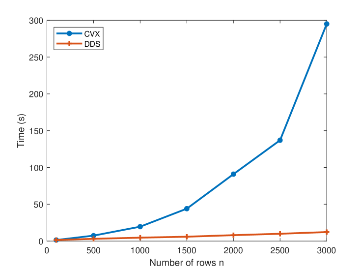
In this subsection, we are going to use DDS to solve problem (134); minimizing nuclear norm of a matrix subject to linear constraints. We are interested in the case that is an -by- matrix with , which makes the s.c. barrier for the epigraph of a matrix norm more efficient than the SDP representation. We compare DDS with convex modeling system CVX, which has a function norm_nuc for nuclear norm. For numerical results, we assume (134) has two linear constraints and and are 0-1 matrices generated randomly. Let us fix the number of columns and calculate the running time by changing the number of rows . Figure 1 shows the plots of running time for both DDS and CVX. For epigraph of a matrix norm constraints, DDS does not form matrices of size , and as can be seen in the figure, the running time is almost linear as a function of . On the other hand, the CVX running time is clearly super-linear.
13.4. Quantum Entropy and Quantum Relative Entropy
In this subsection, we see optimization problems involving quantum entropy. As far as we know, there is no library for quantum entropy and quantum relative entropy functions. We have created examples of combinations of quantum entropy constraints and other types such as LP, SOCP, and -norm. Problems for quantum entropy are of the form
| (269) | |||||
| s.t. | |||||
where and ’s are sparse symmetric matrices. The problems for are also in the same format. Our collection contains both feasible and infeasible cases. The results are shown in Tables 5 and 6 respectively for quantum entropy and quantum relative entropy. The MATLAB files in the DDS format for some of these problems are given in the Test_Examples folder. We compare our results to CVXQUAD, which is a collection of matrix functions to be used on top of CVX. The package is based on the paper [13], which approximates matrix logarithm with functions that an be described as feasible region of SDPs. Note that these approximations increase the dimension of the problem, which is why CVX fails for the larger problems in Table 5.
| Problem | size of | Type of Constraints | Itr/ time(s) | CVXQUAD |
|---|---|---|---|---|
| QuanEntr-10 | QE | 11/ 0.6 | 12/ 1.3 | |
| QuanEntr-20 | QE | 13/ 0.8 | 13/ 2.4 | |
| QuanEntr-50 | QE | 18/ 1.8 | 12/ 23.2 | |
| QuanEntr-100 | QE | 24/ 6.7 | array size error | |
| QuanEntr-200 | QE | 32/ 53.9 | array size error | |
| QuanEntr-LP-10 | QE-LP | 19/ 1.1 | 16/ 3.4 | |
| QuanEntr-LP-20 | QE-LP | 23 / 1.6 | 20/ 9.1 | |
| QuanEntr-LP-50 | QE-LP | 34/ 2.3 | 20/ 103.4 | |
| QuanEntr-LP-100 | QE-LP | 44/ 14.5 | array size error | |
| QuanEntr-LP-SOCP-10-infea | QE-LP-SOCP | 12/ 0.6 (infea) | 16/ 5.1 | |
| QuanEntr-LP-SOCP-10 | QE-LP-SOCP | 26/ 1.0 | 24/ 2.0 | |
| QuanEntr-LP-SOCP-20-infea | QE-LP-SOCP | 14/ 1.1 (infea) | 14/ 5.8 | |
| QuanEntr-LP-SOCP-20 | QE-LP-SOCP | 33/ 1.8 | 22/ 4.1 | |
| QuanEntr-LP-SOCP-100 | QE-LP-SOCP | 51/ 20.8 | array size error | |
| QuanEntr-LP-SOCP-200 | QE-LP-SOCP | 69/ 196 | array size error | |
| QuanEntr-LP-3norm-10-infea | QE-LP-pnorm | 16/ 0.6 (infea) | 22/ 2.0 | |
| QuanEntr-LP-3norm-10 | QE-LP-pnorm | 21/ 1.2 | 19/ 2.0 | |
| QuanEntr-LP-3norm-20-infea | QE-LP-pnorm | 16/ 0.9 (infea) | 18/ 6.5 | |
| QuanEntr-LP-3norm-20 | QE-LP-pnorm | 29/ 1.1 | 20/ 7.3 | |
| QuanEntr-LP-3norm-100-infea | QE-LP-pnorm | 25/ 15.3 (infea) | array size error | |
| QuanEntr-LP-3norm-100 | QE-LP-pnorm | 66/ 40.5 | array size error |
| Problem | size of | Type of Constraints | Itr/ time(s) | CVXQUAD |
|---|---|---|---|---|
| QuanReEntr-6 | QRE | 12/ 6.3 | 12/ 18.1 | |
| QuanReEntr-10 | QRE | 12/ 21.2 | 25/ 202 | |
| QuanReEntr-20 | QRE | 17/ 282 | array size error | |
| QuanReEntr-LP-6 | QRE-LP | 25/ 23.2 | 21/ 19.6 | |
| QuanReEntr-LP-6-infea | QRE-LP | 30/ 11.8 | 28/ 21.5 | |
| QuanReEntr-LP-10 | QRE-LP | 26/ 49.3 | 24/ 223 |
13.5. Hyperbolic Polynomials
We have created a library of hyperbolic cone programming problems for our experiments. Hyperbolic polynomials are defined in Section 10. We discuss three methods in this section for the creation of our library.
13.5.1. Hyperbolic polynomials from matriods
Let us first define a matroid.
Definition 13.1.
A ground set and a collection of independent sets form a matroid if:
-
•
,
-
•
if and , then ,
-
•
if , and , then there exists such that .
The independent sets with maximum cardinality are called the bases of the matroid, we denote the set of bases of the matroid by . We can also assign a rank function as:
| (270) |
Naturally, the rank of a matroid is the cardinality of any basis of it. The basis generating polynomial of a matroid is defined as
| (271) |
A class of hyperbolic polynomials are the basis generating polynomials of certain matroids with the half-plane property [9]. A polynomials has the half-plane property if it is nonvanishing whenever all the variables lie in the open right half-plane. We state it as the following lemma:
Lemma 13.1.
Assume that is a matroid with half-plane property. Then its basis generating polynomial is hyperbolic in any direction in the positive orthant.
Several classes of matroids have been proven to have the half-plane property [9, 3, 1]. As the first example, we introduce the Vamos matroid. The ground set has size 8 (can be seen as 8 vertices of the cube) and the rank of matroid is 4. All subsets of size 4 are independent except 5 of them. Vamos matroid has the half-plane property [37]. The basis generating polynomial is:
where is the elementary symmetric polynomial of degree with variables. Note that elementary symmetric polynomials are hyperbolic in direction of the vector of all ones. Some extensions of Vamos matroid also satisfy the half-plane property [6]. These matroids give the following Vamos-like basis generating polynomials:
| (272) |
Vamos like polynomials in (272) have an interesting property of being counter examples to one generalization of Lax conjecture [4, 6]. Explicitly, there is no power and symmetric matrices such that
| (273) |
In the DDS package, we have created a function
poly = vamos(m)
that returns a Vamos like polynomial as in (272) in the ’monomial’ format, which can be given as cons{k,3} for inputting a hyperbolic constraint. vamos(4) returns the Vamos polynomial with 8 variables.
Graphic matroids also have the half-plane property [9]. However, the hyperbolicity cones arising from graphic matroids are isomorphic to positive semidefinite cones. This can be proved using a classical result that the characteristic polynomial of the bases of graphic matroids is the determinant of the Laplacian (with a row and a column removed) of the underlying graph [5]. Consider a graph and let be the set of all spanning trees of . Then the generating polynomial defined as
| (274) |
is a hyperbolic polynomial. Several matroid operations preserve the half-plane property as proved in [9], including taking minors, duals, and direct sums.
We have created a set of problems with combinations of hyperbolic polynomial inequalities and other types of constraints such as those arising from LP, SOCP, and entropy function.
| Problem | size of | var/deg of | Type of Constraints | Itr/ time(s) |
|---|---|---|---|---|
| Vamos-1 | 8/4 | HB | 7/ 1.5 | |
| Vamos-LP-1 | 8/4 | HB-LP | 8/ 2 | |
| Vamos-SOCP-1 | 8/4 | HB-LP-SOCP | 12/ 2 | |
| Vamos-Entr-1 | 8/4 | HB-LP-Entropy | 9/ 1.2 | |
| VL-Entr-1 | 20/4 | HB-LP-Entropy | 9/ 24 | |
| VL-Entr-1 | 30/4 | HB-LP-Entropy | 12/ 211 |
13.5.2. Derivatives of products of linear forms
Hyperbolicity of a polynomial is preserved under directional derivative operation (see [30]):
Theorem 13.1.
Let be hyperbolic in direction and of degree at least 2. Then the polynomial
| (275) |
is also hyperbolic in direction . Moreover,
| (276) |
Assume that , where are linear forms. Then, is hyperbolic in the direction of any vector such that . As an example, consider . Recursively applying Theorem 13.1 to such polynomials leads to many hyperbolic polynomials, including all elementary symmetric polynomials. For some properties of hyperbolicity cones of elementary symmetric polynomials, see [38]. For some preliminary computational experiments on such hyperbolic programming problems, see [24].
For the polynomials constructed by the products of linear forms, it is more efficient to use the straight-line program. For a polynomial , let us define a -by- matrix where the th row contains the coefficients of . In DDS, we have created a function
[poly,poly_grad] = lin2stl(M,d)
which returns two polynomials in ”straight-line” form, one as the product of linear forms defined by , and the other one its directional derivative in the direction of . For example, if we want the polynomial , then our is defined as
| (279) |
Table 8 shows some results of problem where the hyperbolic polynomial is either a product of linear forms or their derivatives.
| Problem | size of | var/deg of | Type of Constraints | Itr |
|---|---|---|---|---|
| HPLin-LP-1 | 5/3 | HB-LP | 8 | |
| HPLinDer-LP-1 | 5/3 | HB-LP | 7 | |
| HPLin-LP-2 | 5/7 | HB-LP | 19 | |
| HPLinDer-LP-2 | 5/7 | HB-LP | 22 | |
| HPLin-Entr-1 | 10/15 | HB-LP-Entropy | 19 | |
| HPLinDer-Entr-1 | 10/15 | HB-LP-Entropy | 18 | |
| HPLin-pn-1 | 10/15 | HB-LP-pnorm | 30 | |
| HPLinDer-pn-1 | 10/15 | HB-LP-pnorm | 32 | |
| Elem-unb-10 | 10/3 | HB | 12 (unb) | |
| Elem-LP-10 | 10/3 | HB-LP | 9 | |
| Elem-LP-10-2 | 10/3 | HB-LP | 30 | |
| Elem-Entr-10-1 | 10/3 | HB-LP-Entropy | 17 | |
| Elem-Entr-10-2 | 10/4 | HB-LP-Entropy | 18 |
13.5.3. Derivatives of determinant of matrix pencils
Let be Hermitian matrices and be such that is positive definite. Then, is hyperbolic in direction . Now, by using Theorem 13.1, we can generate a set of interesting hyperbolic polynomials by taking the directional derivative of this polynomial up to times at direction .
References
- [1] N. Amini and P. Brändén, Non-representable hyperbolic matroids, Adv. Math., 334 (2018), pp. 417–449.
- [2] S. Boyd, S.-J. Kim, L. Vandenberghe, and A. Hassibi, A tutorial on geometric programming, Optimization and Engineering, 8 (2007), pp. 67–127.
- [3] P. Brändén, Polynomials with the half-plane property and matroid theory, Advances in Mathematics, 216 (2007), pp. 302–320.
- [4] , Obstructions to determinantal representability, Advances in Mathematics, 226 (2011), pp. 1202–1212.
- [5] , Hyperbolicity cones of elementary symmetric polynomials are spectrahedral, Optimization Letters, 8 (2014), pp. 1773–1782.
- [6] S. Burton, C. Vinzant, and Y. Youm, A real stable extension of the vamos matroid polynomial, arXiv preprint arXiv:1411.2038, (2014).
- [7] V. Chandrasekaran and P. Shah, Relative entropy optimization and its applications, Mathematical Programming, 161 (2017), pp. 1–32.
- [8] R. Chares, Cones and Interior-Point Algorithms for Structured Convex Optimization Involving Powers and Exponentials, PhD thesis, Université Catholique de Louvain, Louvain-la-Neuve, 2008.
- [9] Y.-B. Choe, J. G. Oxley, A. D. Sokal, and D. G. Wagner, Homogeneous multivariate polynomials with the half-plane property, Advances in Applied Mathematics, 32 (2004), pp. 88–187.
- [10] J. Dahl and E. D. Andersen, A primal-dual interior-point algorithm for nonsymmetric exponential-cone optimization, Optimization Online, (2019).
- [11] C. Davis, All convex invariant functions of hermitian matrices, Archiv der Mathematik, 8 (1957), pp. 276–278.
- [12] S.-C. Fang, J. R. Rajasekera, and H.-S. J. Tsao, Entropy optimization and Mathematical Programming, vol. 8, Springer Science & Business Media, 1997.
- [13] H. Fawzi, J. Saunderson, and P. A. Parrilo, Semidefinite approximations of the matrix logarithm, Foundations of Computational Mathematics, 19 (2019), pp. 259–296.
- [14] L. Faybusovich and T. Tsuchiya, Matrix monotonicity and self-concordance: how to handle quantum entropy in optimization problems, Optimization Letters, (2017), pp. 1513–1526.
- [15] H. A. Friberg, Cblib 2014: a benchmark library for conic mixed-integer and continuous optimization, Mathematical Programming Computation, 8 (2016), pp. 191–214.
- [16] M. Grant, S. Boyd, and Y. Ye, CVX: MATLAB software for disciplined convex programming, 2008.
- [17] O. Güler, Hyperbolic polynomials and interior point methods for convex programming, Mathematics of Operations Research, 22 (1997), pp. 350–377.
- [18] F. Hiai and D. Petz, Introduction to matrix analysis and applications, Springer Science & Business Media, 2014.
- [19] M. Karimi and L. Tunçel, Primal-dual interior-point methods for Domain-Driven formulations, Mathematics of Operations Research (to appear), arXiv preprint arXiv:1804.06925, (2018).
- [20] , Status determination by interior-point methods for convex optimization problems in domain-driven form, arXiv preprint arXiv:1901.07084, (2019).
- [21] A. S. Lewis, The mathematics of eigenvalue optimization, Mathematical Programming, 97 (2003), pp. 155–176.
- [22] H. D. Mittelmann, The state-of-the-art in conic optimization software, in Handbook on Semidefinite, Conic and Polynomial Optimization, Springer, 2012, pp. 671–686.
- [23] MOSEK ApS, The MOSEK optimization toolbox for MATLAB manual. Version 9.0., 2019. http://docs.mosek.com/9.0/toolbox/index.html.
- [24] T. G. J. Myklebust, On primal-dual interior-point algorithms for convex optimisation, PhD thesis, Department of Combinatorics and Optimization, Faculty of Mathematics, University of Waterloo.
- [25] A. Nemirovski and L. Tunçel, Cone-free primal-dual path-following and potential reduction polynomial time interior-point methods, Mathematical Programming, 102 (2005), pp. 261–294.
- [26] Y. Nesterov, Lectures on Convex Optimization, Springer, 2018.
- [27] Y. Nesterov and A. Nemirovski, Interior-Point Polynomial Algorithms in Convex Programming, SIAM Series in Applied Mathematics, SIAM: Philadelphia, 1994.
- [28] G. Pataki and S. Schmieta, The DIMACS library of semidefinite-quadratic-linear programs, tech. rep., Preliminary draft, Computational Optimization Research Center, Columbia University, New York, 2002.
- [29] B. Recht, M. Fazel, and P. A. Parrilo, Guaranteed minimum-rank solutions of linear matrix equations via nuclear norm minimization, SIAM Review, 52 (2010), pp. 471–501.
- [30] J. Renegar, Hyperbolic programs, and their derivative relaxations, Foundations of Computational Mathematics, 6 (2006), pp. 59–79.
- [31] S. Roy and L. Xiao, On self-concordant barriers for generalized power cones, tech. rep., Tech. Report MSR-TR-2018-3, January 2018, https://www. microsoft. com/en-us …, 2018.
- [32] J. F. Sturm, Using SeDuMi 1.02, a MATLAB toolbox for optimization over symmetric cones, Optimization Methods and Software, 11 (1999), pp. 625–653.
- [33] K.-C. Toh, M. J. Todd, and R. H. Tütüncü, On the implementation and usage of SDPT3–a MATLAB software package for semidefinite-quadratic-linear programming, version 4.0, in Handbook on semidefinite, conic and polynomial optimization, Springer, 2012, pp. 715–754.
- [34] J. Tropp, An introduction to matrix concentration inequalities, arXiv preprint arXiv:1501.01571, (2015).
- [35] L. Tunçel and A. Nemirovski, Self-concordant barriers for convex approximations of structured convex sets, Foundations of Computational Mathematics, 10 (2010), pp. 485–525.
- [36] R. H. Tütüncü, K.-C. Toh, and M. J. Todd, Solving semidefinite-quadratic-linear programs using SDPT3, Mathematical programming, 95 (2003), pp. 189–217.
- [37] D. G. Wagner and Y. Wei, A criterion for the half-plane property, Discrete Mathematics, 309 (2009), pp. 1385–1390.
- [38] Y. Zinchenko, On hyperbolicity cones associated with elementary symmetric polynomials, Optim. Lett., 2 (2008), pp. 389–402.
Appendix A Calculating the predictor and corrector steps
As discussed in [19], for both the predictor and corrector steps, the theoretical algorithm solves a linear system with the LHS matrix of the form
| (286) |
where is a matrix that contains the linear transformations we need:
| (291) |
and are positive definite matrices based on the Hessians of the s.c. functions, is a matrix whose rows form a basis for , is any vector that satisfies , and , , , and are scalars and vectors defined in [19]. A practical issue of this system is that calculating is not computationally efficient, and DDS uses a way around it. If we expand the system given in (286), the linear systems DDS needs to solve become of the form:
At the end, we are interested in to calculate our search directions. If we consider the last equation, we can remove the matrix multiplied from the left to all the terms as
| (293) | |||||
where . Now, we multiply the last equation by from the left and eliminate to get
| (294) |
By using the equations in (293) and (294), we can get a linear system without as
| (304) |
By Sherman–Morrison formula, we can write
| (306) | |||||
Let us define
| (307) |
Then we can see that the LHS matrix in (304) can be written as
| (317) |
This matrix is a -by- matrix plus a rank one update. If we have the Cholesky or LU factorization of and (in the case that , we need just one such factorization), then we have such a factorization for the -by- leading minor of and we can easily extend it to a factorization for the whole . To solve the whole system, we can then use Sherman-Morrison formula.
Appendix B Implementation details for SDP and generalized epigraphs of matrix norms
DDS accepts many constraints that involve matrices. These matrices are given into DDS as vectors. Calculating the derivatives and implementing the required linear algebra operations efficiently is critical in the performance of DDS. In DDS 2.0, many ideas and tricks have been used for matrix functions. In this section, we mention some of these techniques for SDP and matrix norm constraints.
B.1. SDP
The primal and dual barrier functions being used for SDP constraints (53) are:
| (318) |
For function , we have:
| (319) |
To implement our algorithm, for each matrix , we need to find the corresponding gradient and Hessian , such that for any symmetric positive semidefinite matrix and symmetric matrix we have:
| (320) |
It can be shown that and , where stands for the Kronecker product of two matrices. Although this representation is theoretically nice, there are two important practical issues with it. First, it is not efficient to calculate the inverse of a matrix explicitly. Second, forming and storing is not numerically efficient for large scale problems. DDS does not explicitly form the inverse of matrices. An important matrix in calculating the search direction is , where is the s.c. barrier for the whole input problem. In DDS, there exist an internal function hessian_A that directly returns in an efficient way, optimized for all the set constraints, including SDP. For transitions from matrices to vectors, we use the properties of Kronecker product that for matrices , , and of proper size, we have
| (321) |
Similar to hessian_A, there are other internal functions in DDS for efficiently calculating matrix-vector products, such as hessian_V for evaluating the product of Hessian with a given vector of proper size.
B.2. Generalized epigraphs of matrix norms
Proposition B.1.
Proof.
For the proof we use the fact that if , then . Also note that if we define
| (323) |
then
and similarly for . We do not provide all the details, but we show how the proof works. For example, let us define
| (324) |
and we want to calculate . We have
| (325) | |||||
∎
Note that all the above formulas for the derivatives are in matrix form. Let us explain briefly how to convert them to the vector form for the code. We explain it for the derivatives of and the rest are similar. From (B.1) we have
| (326) | |||||
Hence, if is the gradient of in the vector form, we have
| (329) |
The second derivatives are trickier. Assume that for example we want the vector form for . By using (B.1) we can easily get each entry of ; consider the identity matrix of size . If we choose to represent the th column of this identity matrix, we get . Practically, this can be done by a loop, which is not efficient. What we did in the code is to implement this using matrix multiplication.
Appendix C Quantum entropy and quantum relative entropy
The s.c. barrier DDS uses for quantum entropy is given in (210). To derive the LF conjugate, we solve the optimization problem in (211); let us write the first order optimality conditions for (211). Section 3.3 of the book [18] is about the derivation of matrix-values functions. For the first derivative, we have the following theorem:
Theorem C.1.
Let and be self-adjoint matrices and be a continuously differentiable function defined on an interval. Assume that the eigenvalues of are in for an interval around . Then,
| (330) |
The first-order optimality conditions for (211) can be written as
| (331) |
If we substitute the first equation in the second one, we get
| (332) |
This equation implies that and are simultaneously diagonalizable and if we have , then we have and so
| (333) |
Here, we focus on the case that . This matrix function is related to quantum relative entropy and Von-Neumann entropy optimization problems (see [7] for a review of the applications). In this case, we can use results for type 3 univariate function in Table 2 and use the function we defined in (344). The LF conjugate of (211) is given in the following lemma:
Lemma C.1.
Proof.
To implement our primal-dual techniques, we need the gradient and Hessian of and . We already saw in Theorem C.1 how to calculate the gradient. The following theorem gives us a tool to calculate the Hessian.
Theorem C.2 ([18]-Theorem 3.25).
Assume that is a -function and with . Then, for a Hermitian matrix , we have
| (337) |
where is the Hadamard product and is the divided difference matrix:
| (340) |
is diagonal in the statement of the theorem, which is without loss of generality. Note that by the definition of functional calculus in (208), for a Hermitian matrix and a unitary matrix , we have
| (341) |
Therefore, for a matrix , we can update (337)
| (342) |
where we extend the definition of in (340) to non-diagonal matrices. Now we can use Theorems C.2 and C.1 to calculate the Hessian of a matrix function.
Corollary C.1.
Let , , and be self-adjoint matrices and be a continuously differentiable function defined on an interval. Assume that the eigenvalues of and are in for an interval around . Assume that . Then,
| (343) |
Let us calculate the gradient and Hessian for our functions for . Let in the following.
For the second derivative, we can use the fact that
Using this formula, we have ()
Now let us compute the gradient and Hessian for the conjugate function. Let , by using Theorem C.1, the gradient of is
where is the matrix extension of . For the second derivative, let us first define as in (340):
In the expression of the Hessian, we use as the matrix extension of . Then, we have
Appendix D Univariate convex functions
DDS 2.0 uses the epigraph of six univariate convex function, given in Table 2, in the direct sum format to handle important constraints such as geometric and entropy programming. In these section, we show how to calculate the LF conjugate for 2-variable s.c. barriers. Some of these function are implicitly evaluated, but in a computationally efficient way. In the second part of this section, we show that gradient and Hessian of these functions can also be evaluated efficiently.
D.1. Legendre-Fenchel conjugates of univariate convex functions
The LF conjugates for the first three functions are given in Table 9.
| 1 | ||
| 2 | ||
| 3 |
Finding the LF conjugates for the first two functions can be handled with easy calculus. In the third row, , defined in [25], is the unique solution of
| (344) |
It is easy to check by implicit differentiation that
We can calculate with accuracy in few steps with the following Newton iterations:
The s.c. barrier DDS uses for the set , is . To find the LF conjugate, we need to solve the following optimization problem:
| (346) |
By writing the first order optimality conditions we have:
| (347) |
By doing some algebra, we can see that and satisfy:
| (348) |
Let us define as the solution of the first equation in (D.1). For each pair , we can calculate by few iterations of Newton method. Then, the first and second derivative can be calculated in terms of . In DDS, we have two functions for these derivatives.
p1_TD(y,eta,p)    % returns  z
p1_TD_der(y,eta,p)  % returns [z_y  z_eta  z_y,y  z_y,eta  z_eta,eta]
For the set defined by , the corresponding s.c. barrier is . To calculate the LF conjugate, we need to solve the following optimization problem:
| (349) |
By writing the first order optimality conditions we have:
| (350) |
By doing some algebra, we can see that satisfies:
| (351) |
Similar to the previous case, let us define as the solution of the first equation in (351). For each pair , we can calculate by few iterations of Newton method. Then, the first and second derivatives can be calculated in terms of . The important point is that when we calculate , then the derivatives can be calculated by explicit formulas. In our code, we have two functions
p2_TD(y,eta,p)    % returns  z
p2_TD_der(y,eta,p)  % returns [z_y  z_eta  z_y,y  z_y,eta  z_eta,eta]
The inputs to the above functions can be vectors. Table 10 is the continuation of Table 9.
| s.c. barrier | ||
|---|---|---|
| 4 | ||
| 5 |
For the set defined by , the corresponding s.c. barrier is . To calculate the LF conjugate, we need to solve the following optimization problem:
| (352) |
At the optimal solution, we must have
| (353) |
Since we have , then we must have at a dual feasible point. By solving these systems we get
| (354) | |||||
D.2. Gradient and Hessian
In this subsection, we show how to calculate the gradient and Hessian for the s.c. barriers and their LF conjugates. Specifically for the implicit function, we show that the derivatives can also be calculated efficiently. First consider the three pairs of functions in Table 9. Here are the explicit formulas for the first and second derivatives:
For the primal function we have
and for the dual function we have
For the primal function we have
and for the dual function we have
For the primal function we have
For the dual function, since the argument of the function is always , we ignore that in the following formulas and use , , and for the function and its derivative.
where
where is the solution of
| (361) |
For simplicity, we drop the arguments of and denote it as . We denote the first derivatives with respect to and as and , respectively. Similarly, we use , , and for the second derivatives. We have
| (362) |
For calculating the second derivatives of , we need the derivatives of :
| (363) |
Then we have
By the above definitions of , , and , we have
The first and second derivatives of are calculated as follows:
| (367) | |||||
| (371) |
The first and second derivatives of are messier. For the first derivative we have
| (375) |
For calculating the second derivative, we also need the second derivatives of :
Using the second derivatives of , we have
| (379) |
where
and have similar formulations.
where is the solution of
| (380) |
Similar to the previous case, for simplicity, we drop the arguments of and denote it as . We denote the first derivatives with respect to and as and , respectively. By implicit differentiation, we have
For the second derivatives of , by using
we have
The first and second derivatives of are calculated as follows:
The first derivative of is equal to
| (385) |
and the second derivatives of is equal to
| (389) |
where
For the primal function we have
and for the dual function we have
Appendix E A s.c. barrier for vector relative entropy
In section, we prove that the function
| (392) |
is a -LH-s.c. barrier for the epigraph of vector relative entropy function defined as
First note that is -LH, so we just need to prove self-concordance.
The proof is based on the compatibility results of [27]. We first consider the case and then generalize it. Let us define the map as
| (393) |
For a vector , we can verify
| (394) |
(E) implies that is concave with respect to . We claim that is -compatible with the barrier ([27]- Definition 5.1.2). For this, we need to show
| (395) |
By using (E) and canceling out the common terms from both sides, (395) reduces to
| (396) |
We can assume that the LHS is nonnegative, then by taking the square of both side and reordering, we get the obvious inequality
| (397) |
Therefore is -compatible with the barrier . Also note that its summation with a linear term is also -compatible with the barrier . Hence, is a 3-s.c. barrier by [27]-Proposition 5.1.7.
For the general case, consider the map as
| (398) |
For a vector of proper size, we have
| (399) |
We claim that is -compatible with the barrier . First note that is concave with respect to . We need to prove a similar inequality as (395) for . Clearly we have
| (400) |
Using inequality (395) and (400) for all and adding them together yields the inequality we want for . Therefore, is -compatible with the barrier , and by [27]-Proposition 5.1.7, (392) is a -s.c. barrier.
Appendix F Comparison with some related solvers and modeling systems
In this section, we take a look at the input format for some other well-known solvers and modeling systems. [22] is a survey by Mittelmann about solvers for conic optimization, which gives an overview of the major codes available for the solution of linear semidefinite (SDP) and second-order cone (SOCP) programs. Many of these codes also solve linear programs (LP). We mention the leaders MOSEK, SDPT3, and SeDuMi from the list. We also look at CVX, a very user-friendly interface for convex optimization. CVX is not a solver, but is a modeling system that (by following some rules) detects if a given problem is convex and remodels it as a suitable input for solvers such as SeDuMi.
F.1. MOSEK [23]
MOSEK is a leading commercial solver for not just optimization over symmetric cones, but also many other convex optimization problems. The most recent version, MOSEK 9.0, for this state-of-the-art convex optimization software handles, in a primal-dual framework, many convex cone constraints which arise in applications [10]. There are different options for the using platform that can seen in MOSEK’s website [23].
F.2. SDPT3 [36, 33]
SDPT3 is a MATLAB package for optimization over symmetric cones, and it solves a conic optimization problem in the equality form as
| (404) |
where our cone can be a direct sum of nonnegative rays (leading to LP problems), second-order cones or semidefinite cones. The Input for SDPT3 is given in the cell array structure of MATLAB. The command to solve SDPT3 is of he form
[obj,X,y,Z,info,runhist] = sqlp(blk,At,C,b,OPTIONS,X0,y0,Z0).
The input data is given in different blocks, where for the th block, blk{k,1} specifies the type of the constraint. Letters ’l’, ’q’, and ’s’ are representing linear, quadratic, and semidefinite constraints. In the th block, At{k}, C{k}, … contain the part of the input related to this block.
F.3. SeDuMi [32]
SeDuMi is also a MATLAB package for optimization over symmetric cones in the format of (404). For SeDuMi, we give as the input , and and a structure array . The vector of variables has a “direct sum” structure. In other words, the set of variables is the direct sum of free, linear, quadratic, or semidefinite variables. The fields of the structure array contain the number of constraints we have from each type and their sizes. SeDuMi can be called in MATLAB by the command
[x,y] = sedumi(A,b,c,K);
and the variables are distinguished by as follows:
-
(1)
is the number of free variables, i.e., in the variable vector , x(1:K.f) are free variables.
-
(2)
is the number of nonnegative variables.
-
(3)
lists the dimension of Lorentz constraints.
-
(4)
lists the dimensions of positive semidefinite constraints.
For example, if K.l=10, K.q=[3 7] and K.s=[4 3], then x(1:10) are non-negative. Then we have x(11) >= norm(x(12:13)), x(14) >= norm(x(15:20)), and mat(x(21:36),4) and mat(x(37:45),3) are positive semidefinite. To insert our problem into SeDuMi, we have to write it in the format of (404) . We also have the choice to solve the dual problem because all of the above cones are self-dual.
F.4. CVX [16]
CVX is an interface that is more user-friendly than solvers like SeDuMi. It provides many options for giving the problem as an input, and then translates them to an eligible format for a solver such as SeDuMi. We can insert our problem constraint-by-constraint into CVX, but they must follow a protocol called Disciplined convex programming (DCP). DCP has a rule-set that the user has to follow, which allows CVX to verify that the problem is convex and convert it to a solvable form. For example, we can write a constraint only when the left side is convex and the right side is concave, and to do that, we can use a large class of functions from the library of CVX.