Doping-dependent metal-insulator transition in a disordered Hubbard model
Abstract
We study the effect of disorder and doping on the metal-insulator transition in a repulsive Hubbard model on a square lattice using the determinant quantum Monte Carlo method. First, with the aim of making our results reliable, we compute the sign problem with various parameters such as temperature, disorder, on-site interactions, and lattice size. We show that in the presence of randomness in the hopping elements, the metal-insulator transition occurs and the critical disorder strength differs at different fillings. We also demonstrate that doping is a driving force behind the metal-insulator transition.
I Introduction
Metal-insulator transitions are an interesting topic of intense activity in modern physics. In general, there are three kinds of insulators. Systems in which the valence band is completely filled are called band insulatorsFabrizio et al. (1999); Bethe (1928). The staggered potential, in which the on-site energies are different, can also produce band insulators with a spectral gap in cold atom experimentsMesser et al. (2015); Loida et al. (2017). In real materials, disorder weakens the constructive interference and affects quantum transport. Disorder-induced localization, which was proposed more than half a century ago as the Anderson insulator, has inspired numerous efforts to explore the metal-insulator transitionAnderson (1958, 1978); Störzer et al. (2006). In addition to these systems, when electron correlations are considered, a metallic system can become an insulator, induced by the competition between the energy gap and the kinetic energy; the electrons in the narrow bands near the Fermi energy become localized, and the system becomes a Mott insulatorKancharla and Okamoto (2007); RC (1977).
In past decades, the nature of the disorder-driven metal-insulator transition in two dimensional (2D) interacting system has been discussed intensivelyA.M.Finkel’stein (1983, 1984); Castellani et al. (1984, 1998); Punnoose and Finkel’stein (2001, 2005); Shashkin and Kravchenko (2019). The existence of a metal state at zero magnetic filed was firstly predicted by FinkelsteinA.M.Finkel’stein (1983, 1984) and Castellani et alCastellani et al. (1984), and the possibility of metallic behavior and metal-insulator transition were later confirmed in Refs.Punnoose and Finkel’stein (2001); Castellani et al. (1998). By perturbative renormalization group methods, the combined effects of interactions and disorder were studied, and a quantum critical point was identified to separate the metallic phase stabilized by electronic correlation from insulating phase where disorder prevails over the electronic interactionsPunnoose and Finkel’stein (2005). For reviews, see Refs.Shashkin and Kravchenko (2019) and references therein. To understand the metal-insulator transition, it is now believed that we must consider both electronic correlation and disorder on the same footing because disorder and interactions are both present in real materialsCurro (2009); Dagotto (2005); Kravchenko et al. (1994). From a theoretical point of view, this is difficult. When both disorder and interactions are strong, perturbative approaches usually break downBelitz and Kirkpatrick (1994); Castellani et al. (1984), and quantum Monte Carlo simulations may be affected by the ‘minus-sign problem’.
In the context of QMC simulations, various interesting metal-insulator transitions have been reported in different physical systemsMa et al. (2018); Chang and Scalettar (2012); Chen et al. (2020). By studying the disordered Hubbard model on a square lattice at quarter filling, it was shown that repulsion between electrons can significantly enhance the conductivity, which provides evidence of a phase transition, in a two-dimensional model containing both interactions and disorderDenteneer et al. (1999). The effects of a Zeeman magnetic field on the transport and thermodynamic properties have also been discussedDenteneer and Scalettar (2003); it was argued that a magnetic field enhances localized behavior in the presence of interactions and disorder and induces a metal-insulator transition, in which the qualitative features of magnetoconductance agree with experimental findings. In a two-dimensional system of a honeycomb lattice that features a linearly vanishing density of states at the Fermi level, a novel disorder-induced nonmagnetic insulating phase is found to emerge from the zero-temperature quantum critical point, separating a semimetal from a Mott insulatorSingha et al. (2011). The authenticity of the insulating phase has also been studied, and ‘false insulating’ behavior originates in closed-shell effectsMondaini et al. (2012).
However, due to the limitation of the ‘minus-sign problem’ in QMC simulations, most studies have focused on the half-filled caseChiesa et al. (2008); Pezzoli and Becca (2010) or some fixed electronic fillingHenseler et al. (2008); Srinivasan et al. (2003). Experimentally, transport measurements of effectively two-dimensional (2D) electron systems in silicon metal-oxide-semiconductor field-effect transistors provided evidence that a metal-insulator transition can occur, where the temperature dependence of the conductivity changes from that typical of an insulator at lower density to that typical of a conductor as the density increases above a critical densityKravchenko et al. (1994, 1995, 1996). In two-dimensional Mott insulator also observed a transition from an anomalous metal to a Fermi liquid by dopingKoepsell et al. (2021). Thus, doping is also an important physical parameter to tune the phase transition, while determining the doping-dependent metal-insulator transition is a subtle and largely understudied problem. And study reported that cold atom-based quantum simulations offer remarkable opportunity for investigate the doping problemGross and Bloch (2017).
In this paper, we evaluate the doping-dependent sign problem and then select several doping levels to examine the doping-dependent metal-insulator transition of the disordered Hubbard model on a square lattice. We then examine whether this model also has a universal value of conductivity. In simulations, the sign problem is minimized by choosing off-diagonal values rather than diagonal disorder because, at least at half filling, there is no sign problem in the former case, and consequently, simulations can be pushed to significantly lower temperatures. We show that the sign-problem behavior worsens with increasing parameter strength, such as on-site interaction; however, the sign-problem behavior also decreases in the presence of bond disorderUlmke and Scalettar (1997). For results away from half filling, we choose some points, where the sign problem is less severe compared to other densities, and show a phase diagram of the critical disorder strength determined by repulsion and doping in a disordered Hubbard model, going beyond previous resultsDenteneer et al. (1999).
II Model and method
The Hamiltonian for a disordered Hubbard model on a square lattice is defined as
| (1) |
where and represent the hopping amplitude between the nearest-neighbor electrons and on-site repulsive interaction,respectively, and denotes the chemical potential, which can control the electron density of the system. is the creation (annihilation) operator with spin at site , and = is the number operator. Disorder is introduced by taking the hopping parameters from a probability for and zero otherwise. is a measure of the strength of the disorderDenteneer et al. (1999). We set =1 as the default energy scale. The number of disorder realizations used in present work is which is enough to obtain reliable results (see Appendix for details).
We use the DQMC methodBlankenbecler et al. (1981) to investigate the phase transitions in the model defined by Eq.(1) numerically. DQMC is a nonperturbative approach, providing an exact numerical method to study the Hubbard model under a finite temperature. First, the partition function is regarded as a path integral discretized into functions in the imaginary time interval . The kinetic term is quadratic, and the on-site interaction term can be decoupled into a quadratic term by a discrete Hubbard-Stratonovich field; then, by analytically integrating the Hamiltonian quadratic term, can be converted into the product of two fermion determinants, where one is spin up and the other is spin down. The Metropolis algorithm is used to stochastically update the sample, and we set , leading to sufficiently small errors in the Trotter approximation.
To study the phase transitions of the system, we computed the -dependent dc conductivity, which can be obtained from the momentum q- and imaginary time -dependent current-current correlation function Trivedi et al. (1996); Trivedi and Randeria (1995):
| (2) |
Here, =, =, where is the Fourier transform of time-dependent current operator in the direction:
| (3) |
where is the electronic current density operator, defined in Eq.(5).
| (4) |
The validity of Eq.(2) has been examined, and this equation has been used for metal-insulator transitions in the Hubbard model in many studiesTrivedi and Randeria (1995); Denteneer et al. (1999); Ma et al. (2018).
III Results and discussion
At half filling, due to the particle-hole symmetry, under the transformation , the Hamiltonian is unchanged, and the simulation can be performed without considering the sign problemDenteneer et al. (2001). When far from half filling, the system may have a sign problem; thus, in a doped Hubbard model on a square lattice, the notorious sign problem prevents exact results at lower temperatures, at higher interactions, or with larger lattices. To ensure the reliability of the data in our simulation, we first present the average sign in Fig.1, which is shown as a function of electron filling for (a) different temperatures, (b) different interactions, (c) different disorder strengths, and (d) different lattice sizes along with the Monte Carlo parameters after 30,000 iterations. The average sign decays exponentially both with increasing inverse temperature and lattice sizeUlmke and Scalettar (1997).
The average sign is determined by the ratio of the integral of the product of up and down spin determinants to the integral of the absolute value of the productIglovikov et al. (2015):
| (5) |
where is the HS configurations composed of the spatial sites and the imaginary time slices; and is defined as each spin specie matrix. As shown in Fig.1 (a), we evaluate the variation in the sign problem with density for various inverse temperatures. The average sign decreases quickly as the system is doped from to . The average sign is small when , with a value below 0.2 due to the disappearing signal-to-noise ratio in the data, making DQMC simulations nearly impossible. As decreases from 0.68, the average sign increases and then decreases from =0.64 until , after which the average sign continuously increases with decreasing density. Thus, the sign problem is acceptable only at some specific densities, which is correlated with the closed-shell effects. Moreover, comparing various temperatures, the sign problem becomes worse as decreases. Fig.1 (b) shows the effect of the on-site interaction on the sign problem and indicates that the sign problem is more serious with increasing interaction; in other words, the interaction plays a negative role in the average sign. The influence of the bond disorder on the sign problem is shown in Fig.1 (c). By raising the disorder strength, the sign problem improves, fundamentally differing from local site disorder, which breaks the particle-hole symmetryParis et al. (2007) and enhances the sign problem. Fig.1 (d) shows that lattice size also affects the sign problem, and the average sign is smaller for than for .
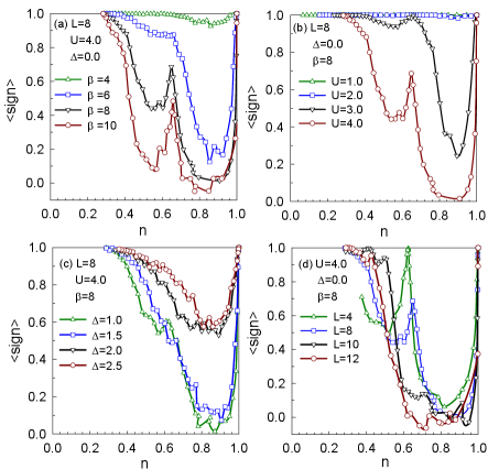
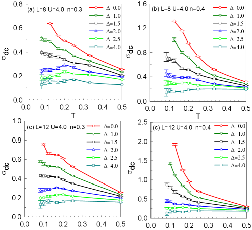
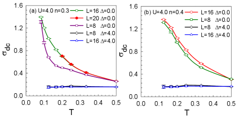
Based on these results, longer runs are required to make the results more reliable. We thus perform simulations where and , in which the sign problem is mild for the DQMC method and does not prohibit obtaining accurate results. In general, in the absence of disorder and frustration, the ground state of the square lattice at half filling is sensitive to interactions, and the system becomes an AF insulator for any finite value of interaction due to the perfect nesting in the Fermi surface. Previous studies demonstrated that when considering disorder at half filling for , the insulating behavior at low temperatures persists to much larger bond disorder strengthsDenteneer et al. (1999). According to previous studies, a basic question arises: On a square lattice with repulsive interactions, in addition to half filling, how are the transport properties at other carrier concentrations affected by disorder? To answer this question, we take advantage of the temperature-dependent dc conductivity to distinguish between an insulator and a metal. Fig.2 shows measured on the square lattice across several disorder values at different densities , where the sign problem has little effect on the results. In the low-temperature regime, the behavior of shows that a transition from metallic to insulating behavior occurs with increasing disorder. For example, when , , and , the dc conductivity grows as the temperature decreases (i.e., ), which indicates that the system is metallic, and the error bars stem from the statistical fluctuation of disorder sampling. Conversely, at , the dc conductivity falls with decreasing temperature (i.e., ) and approaches zero as , which is characteristic of insulating behavior. Therefore, it can be deduced from the above figure that hopping disorder decreases the dc conductivity. The transition from metallic to insulating clearly occurs at . In the same way, by changing the carrier density , the critical disorder strength at is about , indicating the occurrence of the metal-insulator transition in the presence of disorder at other densities, which differs from the half filling case. Fig.2(c), (d) show the results of . Even though the values of dc conductivity have not been saturated at , the values of critical disorder strength are roughly the same for and . Our further data in Fig. 3 (a) show that the dc conductivity itself tends to converge at , while simulations on such lattice cost huge CPU times. And through the shift in the maximum dc conductivity, one can infer that the mobility gap increases as the bond disorder increases.
In addition, we ascertain that the occurrence of a phase transition results from the bond disorder rather than the system size being smaller than a localization length. Fig.3 (a) shows that as the lattice size increases, the dc conductivity will converge to a finite value under various conditions, although the convergence speed is affected by parameter sets (such as in the insulating phase converges faster than in the metallic phase, or in system at converges faster than ).
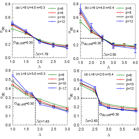
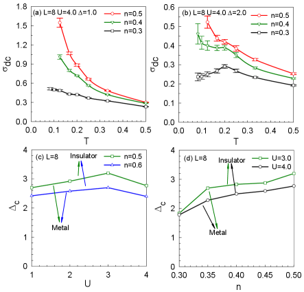
On the basis of Fig.2, we plot as a function of the disorder strength in Fig.4, to determine the critical point accurately and the corresponding value of dc conductivity. The intersection of four curves marks the critical point for the metal-insulator transition. The ordinate of this intersection describes the critical dc conductivity (i.e., at , , and at , ). Here, the value of the critical dc conductivity is determined to an accuracy of 0.01. Comparing the results for these parameters sets ( and ), it shows that the system has the possibility of a universal value of the critical dc conductivity. To strongly support these findings, we present the same plots for different interaction strength () shown in Fig.4 (c) and (d): although the critical disorder strength is varied, the critical dc conductivity is still . Besides, we also compute other parameter sets, such as , , , ; , , , ; , , , ; and , , , . The standard deviation equal to is small enough to ensure the clustering of the dc conductivity values around the mean value, which confirms the existence of universal conductivity()Chakraborty et al. (2011a) (the error 0.01 is computed by estimating the arithmetic mean from the listed eight datasets) and its independence with , , and . This property has also been realized in the quantum sigma modelAnissimova et al. (2007); Punnoose and Finkel’stein (2005), and discussed in both grapheneOstrovsky et al. (2007) and integer quantum Hall effectSchweitzer and Markoš (2005).
To describe the role of doping in more details, we investigate the change in with different densities at fixed disorder strength, as shown in Fig.5 (a) and (b). Increasing the electronic density shall enhance the dc conductivity, and when , the system behaves as an insulator at . Conversely, at and , the system behaves as a metal. Thus, we deduce that doping can affect the metal-insulator transition. We compile the results of in Fig.5 (c), (d), showing the relationship between critical disorder strength and interaction strength (or density ). The critical disorder strength increases firstly and then decreases as increases at a fixed density, which is also reported in the ionic Hubbard modelParis et al. (2007); Adibi et al. (2019). The Coulomb repulsion enhances metallicity when , and a larger will make it more effective to localize electrons to decrease . On the other hand, in our calculation, the effect of density on is non-monotonous: increases as the density increases from 0.3 to 0.5, and then decreases as the density increases to 0.6. Although the sign problem restricts us to calculate the large density, the current results have provided strong support for the conclusion that doping-dependent metal-insulator transition in a disordered Hubbard model.
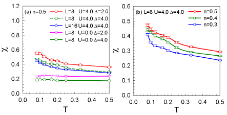
The spin dynamics of electrons are often discussed together with the localization transition, and we discuss the correlation between the spin susceptibility and temperature through , where denotes the ferromagnetic structure factorLiang et al. (1999). Fig.6 (a) shows that the spin susceptibility increases as the temperature decreases and as increases (for and ), meaning that interaction can enhance the ferromagnetic susceptibility. Additionally, the spin susceptibility diverges as , implying that magnetic order exists in both the metallic () and insulating phases (). The ferromagnetic susceptibility reduces with increasing disorder in the presence of interaction and hopping disorder, which is in accord with the Stoner criterion for a ferromagnetic . represents the density of states at the Fermi level. The Stoner criterion estimates that the behavior of a ferromagnetic acts against increasing disorder due to the reduction in the spectral density at the Fermi levelChakraborty et al. (2011b). Comparing the results of with , the spin susceptibility is little affected by size effects. Additionally, we find that the density plays a positive role in the ferromagnetic susceptibility, as shown in Fig.6 (b).
IV Conclusions
In summary, we have studied a disordered Hubbard model on a square lattice away from half filling by using the determinant quantum Monte Carlo method. We find that the sign problem emerges away from half filling, accompanied by a nonmonotonic behavior as the density varies, and that adding hopping disorder can reduce the sign problem. The system becomes metallic at finite unlike with half filling, and the metal-insulator transition is affected by disorder. Although the critical disorder strength non-monotonically varies with changing the electron density and repulsion, the critical dc conductivity is independent of the parameter set, similar to the site disorder caseChakraborty et al. (2011a). The behavior of spin susceptibility suggests that under a range of densities, the insulating phase is accompanied by local moments. The ferromagnetic susceptibility tends to reduce with increasing bond disorder strength, in line with the Stoner criterion.
At fixed disorder, we also demonstrate that the carrier density can be used as a tuning parameter for the occurrence of the phase transition, which can be explained as follows: varying the intensity of disorder at a fixed density can be regarded as adjusting the mobility boundary via the Fermi energy and is similar to varying the carrier concentration at a fixed disorder strength , which can be thought of as a shift in the Fermi energyDenteneer et al. (1999).
Acknowledgements.
This work is supported by NSFC (Nos. 11974049 and 11774033) and Beijing Natural Science Foundation (No. 1192011). The numerical simulations were performed at the HSCC of Beijing Normal University and on the Tianhe-2JK in the Beijing Computational Science Research Center.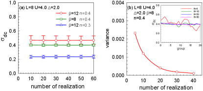
Appendix A Concerning the number of disorder realizations
In general, the required number of disorder realizations must be determined empirically, and is a complex interplay between “self-averaging” on sufficiently large lattices, the strength of the disorder, and the location in the phase diagram. In Fig.7, we show the change of the average dc conductivity with the number of random disorder realizations. For any given density , no change in the average for realization numbers larger than 10. It justifies our usage of realizations in the main text.
We also use the variance to justify our choice of the number of disorder realizations. In the inset of Fig.7 (b), we calculated the average values of several groups of data whose realizations are 5, 10, 20, 30 respectively, and performed 20 times. It can be seen that the average values of each group with N=5 vary greatly and the curve fluctuates violently, means that N=5 can not eliminate the random error well. When the number in a group increased to be 10, fluctuations were significantly suppressed; increased to be 20, the curve tends to be stable. This phenomenon is also shown in Fig.7 (b) in the form of variance of each curve. The variance curve shows good convergence. As the number in a group increases to be 20, the variance has decreased to a value close to 0. That is, 20 times is large enough as the number of realization.
References
- Fabrizio et al. (1999) M. Fabrizio, A. O. Gogolin, and A. A. Nersesyan, Phys. Rev. Lett. 83, 2014 (1999).
- Bethe (1928) H. Bethe, Annalen der Physik 392, 55 (1928).
- Messer et al. (2015) M. Messer, R. Desbuquois, T. Uehlinger, G. Jotzu, S. Huber, D. Greif, and T. Esslinger, Phys. Rev. Lett. 115, 115303 (2015).
- Loida et al. (2017) K. Loida, J.-S. Bernier, R. Citro, E. Orignac, and C. Kollath, Phys. Rev. Lett. 119, 230403 (2017).
- Anderson (1958) P. W. Anderson, Phys. Rev. 109, 1492 (1958).
- Anderson (1978) P. W. Anderson, Rev. Mod. Phys. 50, 191 (1978).
- Störzer et al. (2006) M. Störzer, P. Gross, C. M. Aegerter, and G. Maret, Phys. Rev. Lett. 96, 063904 (2006).
- Kancharla and Okamoto (2007) S. S. Kancharla and S. Okamoto, Phys. Rev. B 75, 193103 (2007).
- RC (1977) RC, Journal of Molecular Structure 38, 297 (1977).
- A.M.Finkel’stein (1983) A.M.Finkel’stein, Sov.Phys.JETP 57, 97 (1983).
- A.M.Finkel’stein (1984) A.M.Finkel’stein, Zeitschrift für Physik B Condensed Matter 56, 189 (1984).
- Castellani et al. (1984) C. Castellani, C. Di Castro, P. A. Lee, and M. Ma, Phys. Rev. B 30, 527 (1984).
- Castellani et al. (1998) C. Castellani, C. Di Castro, and P. A. Lee, Phys. Rev. B 57, R9381 (1998).
- Punnoose and Finkel’stein (2001) A. Punnoose and A. M. Finkel’stein, Phys. Rev. Lett. 88, 016802 (2001).
- Punnoose and Finkel’stein (2005) A. Punnoose and A. M. Finkel’stein, Science 310, 289 (2005).
- Shashkin and Kravchenko (2019) A. A. Shashkin and S. V. Kravchenko, Applied Sciences 9 (2019).
- Curro (2009) N. J. Curro, Reports on Progress in Physics 72, 026502 (2009).
- Dagotto (2005) E. Dagotto, Science 309, 257 (2005).
- Kravchenko et al. (1994) S. V. Kravchenko, G. V. Kravchenko, J. E. Furneaux, V. M. Pudalov, and M. D’Iorio, Phys. Rev. B 50, 8039 (1994).
- Belitz and Kirkpatrick (1994) D. Belitz and T. R. Kirkpatrick, Rev. Mod. Phys. 66, 261 (1994).
- Ma et al. (2018) T. Ma, L. Zhang, C.-C. Chang, H.-H. Hung, and R. T. Scalettar, Phys. Rev. Lett. 120, 116601 (2018).
- Chang and Scalettar (2012) C.-C. Chang and R. T. Scalettar, Phys. Rev. Lett. 109, 026404 (2012).
- Chen et al. (2020) W. Chen, Y. Chu, T. Huang, and T. Ma, Phys. Rev. B 101, 155413 (2020).
- Denteneer et al. (1999) P. J. H. Denteneer, R. T. Scalettar, and N. Trivedi, Phys. Rev. Lett. 83, 4610 (1999).
- Denteneer and Scalettar (2003) P. J. H. Denteneer and R. T. Scalettar, Phys. Rev. Lett. 90, 246401 (2003).
- Singha et al. (2011) A. Singha, M. Gibertini, B. Karmakar, S. Yuan, M. Polini, G. Vignale, M. I. Katsnelson, A. Pinczuk, L. N. Pfeiffer, K. W. West, and V. Pellegrini, Science 332, 1176 (2011).
- Mondaini et al. (2012) R. Mondaini, K. Bouadim, T. Paiva, and R. R. dos Santos, Phys. Rev. B 85, 125127 (2012).
- Chiesa et al. (2008) S. Chiesa, P. B. Chakraborty, W. E. Pickett, and R. T. Scalettar, Phys. Rev. Lett. 101, 086401 (2008).
- Pezzoli and Becca (2010) M. E. Pezzoli and F. Becca, Phys. Rev. B 81, 075106 (2010).
- Henseler et al. (2008) P. Henseler, J. Kroha, and B. Shapiro, Phys. Rev. B 77, 075101 (2008).
- Srinivasan et al. (2003) B. Srinivasan, G. Benenti, and D. L. Shepelyansky, Phys. Rev. B 67, 205112 (2003).
- Kravchenko et al. (1995) S. V. Kravchenko, W. E. Mason, G. E. Bowker, J. E. Furneaux, V. M. Pudalov, and M. D’Iorio, Phys. Rev. B 51, 7038 (1995).
- Kravchenko et al. (1996) S. V. Kravchenko, D. Simonian, M. P. Sarachik, W. Mason, and J. E. Furneaux, Phys. Rev. Lett. 77, 4938 (1996).
- Koepsell et al. (2021) J. Koepsell, D. Bourgund, P. Sompet, S. Hirthe, A. Bohrdt, Y. Wang, F. Grusdt, E. Demler, G. Salomon, C. Gross, and I. Bloch, Science 374, 82 (2021).
- Gross and Bloch (2017) C. Gross and I. Bloch, Science 357, 995 (2017).
- Ulmke and Scalettar (1997) M. Ulmke and R. T. Scalettar, Phys. Rev. B 55, 4149 (1997).
- Blankenbecler et al. (1981) R. Blankenbecler, D. J. Scalapino, and R. L. Sugar, Phys. Rev. D 24, 2278 (1981).
- Trivedi et al. (1996) N. Trivedi, R. T. Scalettar, and M. Randeria, Phys. Rev. B 54, R3756 (1996).
- Trivedi and Randeria (1995) N. Trivedi and M. Randeria, Phys. Rev. Lett. 75, 312 (1995).
- Denteneer et al. (2001) P. J. H. Denteneer, R. T. Scalettar, and N. Trivedi, Phys. Rev. Lett. 87, 146401 (2001).
- Iglovikov et al. (2015) V. I. Iglovikov, E. Khatami, and R. T. Scalettar, Phys. Rev. B 92, 045110 (2015).
- Paris et al. (2007) N. Paris, K. Bouadim, F. Hebert, G. G. Batrouni, and R. T. Scalettar, Phys. Rev. Lett. 98, 046403 (2007).
- Chakraborty et al. (2011a) P. B. Chakraborty, K. Byczuk, and D. Vollhardt, Phys. Rev. B 84, 035121 (2011a).
- Anissimova et al. (2007) S. Anissimova, S. V. Kravchenko, A. Punnoose, A. M. Finkel’stein, and T. M. Klapwijk, Nature Physics 3, 707 (2007).
- Punnoose and Finkel’stein (2005) A. Punnoose and A. M. Finkel’stein, Science 310, 289 (2005).
- Ostrovsky et al. (2007) P. M. Ostrovsky, I. V. Gornyi, and A. D. Mirlin, Phys. Rev. Lett. 98, 256801 (2007).
- Schweitzer and Markoš (2005) L. Schweitzer and P. Markoš, Phys. Rev. Lett. 95, 256805 (2005).
- Adibi et al. (2019) E. Adibi, A. Habibi, and S. A. Jafari, Phys. Rev. B 99, 014204 (2019).
- Liang et al. (1999) S.-D. Liang, Z. D. Wang, Q. Wang, and S.-Q. Shen, Phys. Rev. B 59, 3321 (1999).
- Chakraborty et al. (2011b) P. B. Chakraborty, K. Byczuk, and D. Vollhardt, Phys. Rev. B 84, 155123 (2011b).