Double exponential quadrature for fractional diffusion

Alexander Rieder Fakultät für Mathematik, University of Vienna, 1090 Vienna, Austria, alexander.rieder@univie.ac.at

(August 6, 2025)

Abstract

We introduce a novel discretization technique for both elliptic and parabolic fractional diffusion problems based on double exponential quadrature formulas and the Riesz-Dunford functional calculus. Compared to related schemes, the new method provides faster convergence with fewer parameters that need to be adjusted to the problem. The scheme takes advantage of any additional smoothness in the problem without requiring a-priori knowledge to tune parameters appropriately. We prove rigorous convergence results for both, the case of finite regularity data as well as for data in certain Gevrey-type classes. We confirm our findings with numerical tests.

1 Introduction

The study of processes governed by fractional linear operators has gathered significant interest over the last few years [BV16, V1́7, LPGea20] with applications ranging from physics [AB17b] to image processing [GH15, GO08, AB17b], inverse problems [KR19] and more. See [SZB⁺18] for an overview of applications in different fields.

There are multiple (non-equivalent) ways of defining fractional powers of operators. We mention the integral fractional Laplacian and the spectral definition [LPGea20]. In this paper, we focus the spectral definition which is equivalent to the functional calculus definition.

For discretization of such problems, both stationary and time dependent, multiple approaches have been presented. A summary of the most common can be found in [BBN⁺18, LPGea20]. They can be broadly distinguished into three categories. First, there are approaches which try to apply the methods of finite- and boundary element methods to integral formulation of the fractional Laplacian [AB17a, ABH19]. The second class of methods uses the Caffarelli-Silvestre extension to reformulate the problem as a PDE posed in one additional spatial dimension. This problem is then treated by standard finite element techniques [NOS15a, NOS15b, NOS16, BMN⁺18, MPSV18, MMR20]. The third big class of discretization schemes, and the one our new scheme is part of, was first introduced in [BP15] and later extended to more general operators [BLP19] and time dependent problems [BLP17b, BLP17a, MR21]. They are based on the Riesz-Dunford calculus (sometimes also referred to as Dunford-Taylor or Riesz-Taylor) and employ a $\operatorname{sinc}$ quadrature scheme to discretize the appearing contour integral. $\operatorname{sinc}$ quadrature, and overall $\operatorname{sinc}$ -based numerical methods are less well known than their polynomial based counterparts, but provide rapidly converging schemes [Ste93, LB92] with very easy implementation. The quadrature relies on appropriate coordinate transforms in order to yield analytic, rapidly decaying integrands over the real line and then discretization using the trapezoidal quadrature rule. In [TM74] it was realized that by adding an additional $\sinh$ -transformation, it is possible to get an even faster convergence for certain integrals, namely instead of convergence of the form $e^{-\sqrt{\mathcal{N}_{\textrm{q}}}}$ , it is possible to get rid of the square root and obtain rates of the form $e^{-\frac{\mathcal{N}_{\textrm{q}}}{\ln{\mathcal{N}_{\textrm{q}}}}}$ . Further developments in this direction are summarized in [Mor91]. Such schemes are commonly referred to as double exponential quadrature or $\sinh$ - $\operatorname{tanh}$ quadrature.

In this paper we investigate whether the discretization of the Riesz-Dunford integral can benefit from using a double exponential quadrature scheme instead of the more established $\operatorname{sinc}$ -quadrature. We present a scheme that retains all the advantages of [BLP19, BLP17b, BLP17a] while delivering improved convergence rates. Namely, the scheme is very easy to implement if a solver for elliptic finite element problems is available. It is almost trivially parallelizable, as the main cost consists of solving a series of independent elliptic problems. In addition, it provides (compared to $\operatorname{sinc}$ -methods) superior accuracy over a wide range of applications and does not require subtle tweaking of parameters in order to get good performance. Instead it will automatically pick up any additional smoothness of the underlying problem to give improved convergence. Since for each quadrature point an elliptic FEM problem needs to be solved, reducing the number of quadrature points greatly increases performance of the overall method.

The paper is structured as follows. After fixing the model problem and notation in Section 1.1, Section 2 introduces the double exponential formulas in an abstract way and we collect some known properties. In addition, we provide one small convergence result which, to our knowledge, has not yet appeared in the literature; we show that the double exponential formulas at least provide comparable convergence of order $e^{-\sqrt{\mathcal{N}_{\textrm{q}}}}$ even without requiring additional analyticity compared to standard $\operatorname{sinc}$ methods. In Section 3, we look at the case of a purely elliptic problem without time dependence. It will showcase the techniques used and provide the building block for the more involved problems later on. In Section 4, we then consider what happens if we move into the time-dependent regime. Section 5 provides extensive numerical evidence supporting the theory. We also compare our new method to the standard $\operatorname{sinc}$ -based methods. Finally, Appendix A collects some properties of the coordinate transform involved. The proofs and calculations are elementary but somewhat lengthy and thus have been relegated to the appendix in order to not impact readability of the article.

Throughout this work we will encounter two types of error terms. For those of the form $e^{-\frac{\gamma}{k}}$ we will be content with not working out the constants $\gamma$ explicitly. For the more important terms of the form $e^{-\frac{\gamma^{\prime}}{\sqrt{k}}}$ we will derive explicit constants $\gamma^{\prime}$ which prove sharp in several examples of Section 5.

We close with a remark on notation. Throughout this text, we write $A\lesssim B$ to mean that there exists a constant $C>0$ , which is independent of the main quantities of interest like number of quadrature points $\mathcal{N}_{\textrm{q}}$ or step size $k$ such that $A\leq CB$ . The detailed dependencies of $C$ are specified in the context. We write $A\sim B$ to mean $A\lesssim B$ and $B\lesssim A$ .

Acknowledgments:

The author would like to thank J. M. Melenk for the many fruitful discussions on the topic. Financial support was provided by the Austrian Science Fund (FWF) through the special research program “Taming complexity in partial differential systems” (grant SFB F65) and the project P29197-N32.

1.1 Model problem and notation

In this paper, we consider problems of applying holomorphic functions $f$ to self-adjoint operators, for example the Laplacian. The two large classes of problems treated in this paper stem from the study of fractional diffusion problems, both in the stationary as well as in the transient version. Given a bounded Lipschitz domain $\Omega$ , we consider the self adjoint operator

\mathcal{L}u:=-\operatorname{div}(\mathfrak{A}\nabla u)+\mathfrak{c}u,

where $\mathfrak{A}\in L^{\infty}(\Omega;\mathbb{R}^{d\times d})$ is uniformly SPD and $\mathfrak{c}\in L^{\infty}(\Omega)$ satisfies $\mathfrak{c}\geq 0$ almost everywhere. Unless otherwise specified, the domain $\operatorname{dom}(\mathcal{L})$ is always taken to include homogeneous Dirichlet boundary conditions.

Given the eigenvalues and eigenfunctions of $\mathcal{L}$ equipped with homogeneous Dirichlet boundary conditions denoted by $(\lambda_{j},v_{j})_{j=0}^{\infty}$ , we define the spaces

\displaystyle\mathbb{H}^{\beta}(\Omega):=\Big{\{}u\in L^{2}(\Omega):\left\|u\right\|_{\mathbb{H}^{\beta}(\Omega}<\infty\Big{\}}\qquad\text{with}\qquad\left\|u\right\|_{\mathbb{H}^{\beta}(\Omega)}:=\sum_{j=0}^{\infty}{\lambda_{j}^{\beta}\left|(u,v_{j})_{L^{2}(\Omega)}\right|^{2}}.

(1.1)

One natural way of defining a functional calculus for the operator $\mathcal{L}$ is based on the spectral decomposition.

Definition 1.1 (Spectral calculus).

Let $\mathcal{O}\subseteq\mathbb{R}_{+}$ such that $\sigma(\mathcal{L})\subseteq\mathcal{O}$ . Let $g:\mathcal{O}\to\mathbb{C}$ be continuous with $\left|g(z)\right|\lesssim(1+\left|z\right|)^{\mu}$ for $\mu\in\mathbb{R}$ . We define for $u\in\mathbb{H}^{2\mu}(\Omega)$ :

\displaystyle g(A)u:=\sum_{j=0}^{\infty}{g(\lambda_{j})\big{(}u,v_{j}\big{)}_{L^{2}(\Omega)}\,v_{j}}.

An alternative definition for holomorphic functions, which will prove more useful for approximation is given in the following Definition. It can be shown, see also [BLP17a, Section 2], that the operators resulting from Definition 1.1 and Definition 1.2 coincide.

Definition 1.2 (Riesz-Dunford calculus).

Fix parameters $\sigma\in\{1/2,1\}$ , $\theta\geq 1$ and $\kappa>0$ . Let $\mathcal{O}\subseteq\mathbb{C}$ such that $\mathbb{C}_{+}:=\{z\in\mathbb{C}:\operatorname{Re}(z)>0\}\subseteq\mathcal{O}$ . Let $g:\mathcal{O}\to\mathbb{C}$ be holomorphic with $\left|g(z)\right|\lesssim(1+\left|z\right|)^{-\mu}$ for $\mu\geq 0$ . We define

\displaystyle g(A):=\frac{1}{2\pi i}\int_{\mathcal{C}}{g(z)\big{(}\mathcal{L}-z\big{)}^{-1}\,dz},

(1.2)

where the integral is taken in the sense of Riemann, and $\mathcal{C}$ is the smooth path

\mathcal{C}:=\Big{\{}\kappa\big{(}\cosh(\sigma w)+\theta\sinh(w)\big{)}\quad\text{ for }w\in\mathbb{R}\Big{\}}.

The parameter $\kappa>0$ is taken sufficiently small such that the spectrum of $\mathcal{L}$ satisfies $\kappa<\sigma(\mathcal{L})$ .

Remark 1.3.

The choice of path in Definition 1.2 is somewhat arbitrary. It is only required to encircle the spectrum of $\mathcal{L}$ with winding number $1$ . Throughout this paper, we will only ever use the same path and thus make it part of our definition.

Remark 1.4.

All our results easily generalize to more general positive definite and self-adjoint operators $\mathcal{L}$ over a general Hilbert space $\mathcal{X}$ , as long as an eigen-decomposition is available. The $\mathbb{H}^{\beta}$ -norms in (1.1) are then defined using the $\mathcal{X}$ inner product.

2 Double exponential formulas

In this section, we analyze the quadrature error when applying a double exponential formula for discretizing certain integrals. The main role will be played by the following coordinate transform:

\displaystyle\psi_{\theta,\sigma}(y):=\kappa\Big{[}\cosh\Big{(}\frac{\sigma\pi}{2}\sinh(y)\Big{)}+i\theta\sinh\Big{(}\frac{\pi}{2}\sinh(y)\Big{)}\Big{]}.

(2.1)

We will focus on the cases $\sigma\in\big{\{}\frac{1}{2},1\big{\}}$ and $\theta\geq 1$ . $\kappa$ is again taken sufficiently small as in Definition 1.2.

For $\theta\geq 1$ , $\delta>0$ we define the sets

\displaystyle D_{d(\theta)}:=\Big{\{}z\in\mathbb{C}:\left|\operatorname{Im}(z)\right|<d(\theta)\Big{\}},\qquad\text{and}\qquad D^{\mathrm{exp}}_{\delta}:=\Big{\{}z\in\mathbb{C}:\left|\operatorname{Im}(z)\right|<\delta e^{-\left|\operatorname{Re}(z)\right|}\Big{\}},

(2.2)

where for each $\theta$ , $d(\theta)$ is a constant which is assumed sufficiently small.

Since all the proofs analyzing the properties of $\psi_{\sigma,\theta}$ are elementary but somewhat lengthy and cumbersome, they have been relegated to Appendix A. The most important properties are, that $y\mapsto\psi_{\sigma,\theta}(y)$ for $y\in\mathbb{R}$ traces the contour in the definition of the Riesz Dunford calculus (see Definition 1.2), and that it is analytic in $D_{d(\theta)}$ . The other important results concern the points where $\psi_{\sigma,\theta}$ crosses the real axis, as these points correspond to (possible) poles in the integrand of Definition 1.2. The location of these points, as well as other important estimates are collected in Lemma A.8. Roughly summarizing, the finitely many points satisfying $\psi_{\sigma,\theta}(y)=\lambda$ have distance $1/\ln(\lambda)$ from the real axis. Away from such points $\left|\psi_{\sigma,\theta}(y)-\lambda\right|\gtrsim\lambda$ holds and for $y\to\pm\infty$ the function $\psi_{\sigma,\theta}$ behaves doubly-exponential (Lemma A.4).

Because the quadrature operator will be the main workhorse, we introduce the following notation:

Definition 2.1.

Let $\mathcal{L}$ be a linear (possibly unbounded) operator on a Banach space $\mathcal{X}$ and $\mathcal{O}\subseteq\mathbb{C}$ such that $\mathbb{C}_{+}\subseteq\mathcal{O}$ . For $g:\mathcal{O}\to\mathbb{C}$ holomorphic as in Definition 1.2, $k\geq 0$ and $\mathcal{N}_{\textrm{q}}\in\mathbb{N}\cup\{\infty\}$ we write

\displaystyle Q^{\mathcal{L}}(g,\mathcal{N}_{\textrm{q}})u

\displaystyle:=\frac{1}{2\pi i}\sum_{j=-\mathcal{N}_{\textrm{q}}}^{\mathcal{N}_{\textrm{q}}}{g(\psi_{\sigma,\theta}(jk))\psi_{\sigma,\theta}^{\prime}(jk)(\mathcal{L}-\psi_{\sigma,\theta}(jk))^{-1}u}\qquad\forall u\in\mathcal{X}

(2.3)

and $Q^{\mathcal{L}}(g):=Q^{\mathcal{L}}(g,\infty)$ for the case where no cutoff is performed. The quadrature error will be denoted by

\displaystyle E^{\mathcal{L}}(g,\mathcal{N}_{\textrm{q}})

\displaystyle:=g(\mathcal{L})u-Q^{\mathcal{L}}(g,\mathcal{N}_{\textrm{q}})u,\qquad\forall u\in\operatorname{dom}(g(\mathcal{L}))

(2.4)

where $g(\mathcal{L})$ is given via the Riesz-Dunford integral 1.2. Again, we write $E^{\mathcal{L}}(g):=E^{\mathcal{L}}(g,\infty)$ .

Remark 2.2.

In Definition 2.1, we will often work with the special case $\mathcal{L}=\lambda$ or $\mathcal{L}=\lambda\mathrm{I}$ for $\lambda\in\mathbb{R}$ . For simplicity, in both cases we write $Q^{\lambda}(g,\mathcal{N}_{\textrm{q}})$ , $E^{\lambda}(g,\mathcal{N}_{\textrm{q}})$ etc. It will be clear from context whether the scalar or operator valued operation is needed.

2.1 Abstract analysis of $\operatorname{sinc}$ -quadrature

In this section, we collect some results on $\operatorname{sinc}$ -quadrature formulas.

Remark 2.3.

As is common in the literature, we define the $\operatorname{sinc}$ function as

\operatorname{sinc}(\zeta):=\begin{cases}\frac{\sin(\pi\zeta)}{\pi\zeta}&\zeta\neq 0\\ 1&\zeta=0.\end{cases}

The following result is the main work-horse when analyzing $\operatorname{sinc}$ -quadrature schemes. In order to reduce the required notation, we use a simplified version of [Ste93, Problem 3.2.6].

Proposition 2.4 (Bialecki, see [Ste93, Problem 3.2.6 and Theorem 3.1.9]).

We make the following assumptions on $g$ :

(i)

$g$ is a meromorphic function on the infinite strip $D_{d(\theta)}$ . It is also continuous on $\partial D_{d(\theta)}$ . The poles $\big{(}p_{\ell}\big{)}_{\ell=1}^{N_{p}}$ are all simple and located in $D_{d(\theta)}\setminus\mathbb{R}$ .
(ii)

There exists a constant $C>0$ independent of $y\in\mathbb{R}$ such that for sufficiently large $y>0$ ,

$\displaystyle\int_{-d(\theta)}^{d(\theta)}{\left|g(y+iw)\right|\,dw}$ $\displaystyle\leq C.$ (2.5)

(iii)

We have

\displaystyle N(g,D_{d(\theta)}):=\int_{-\infty}^{\infty}{\left|g(y+id(\theta)\right|+\left|g(y-id(\theta))\right|\,dy}<\infty.

(2.6)

Denote by $\operatorname{res}(g;p_{\ell})$ the residue of $g$ at $p_{\ell}$ , and define $\gamma(k;p_{\ell}):=\frac{1}{\sin(\pi p_{\ell}/k)}.$

Then there exists a generic constant, such that for all $k>0$ , using $s_{\ell}:=\operatorname{sign}(p_{\ell})$ :

\displaystyle\left|\int_{\mathbb{R}}{g(t)\,dt}-k\sum_{n=-\infty}^{\infty}{g(k\,n)}-\pi\sum_{\ell=1}^{N_{p}}{e^{i\frac{s_{\ell}\pi p_{\ell}}{k}}\operatorname{res}(g;p_{\ell})\gamma(k;p_{\ell})}\right|

\displaystyle\lesssim\frac{e^{-2\pi d(\theta)/k}}{1-e^{-2\pi d(\theta)/k}}N(g,D_{d(\theta)}).

(2.7)

Proposition 2.4 requires certain decay properties for the integrand in a complex strip, and thus is not always applicable. As is shown in Appendix A, the transformation $\psi_{\sigma,\theta}$ maps partly into the left-half plane. One can even show that the real part changes sign infinitely many times when evaluating along a line of fixed imaginary part. If we therefore consider the case when $f(z):=e^{-z}$ is the exponential function, this means that $f\circ\psi$ is exponentially increasing in such regions. This puts showing estimates of the form required in Proposition 2.4 (iii) out of reach.

On the other hand, Lemma A.5 shows that for $\sigma=1$ , restricted to the domain $D^{\mathrm{exp}}_{\delta}$ , the map $\psi_{\sigma,\theta}$ stays in the right half-plane. Here the exponential function is decreasing. Similarly, the Mittag-Leffler function $e_{\alpha,\mu}$ is decreasing on slightly larger sectors, allowing for the choice of $\sigma=1/2$ if $\alpha<1$ . This motivates the following modification of Proposition 2.4.

Lemma 2.5.

Assume that $g:D^{\mathrm{exp}}_{\delta}\to\mathbb{C}$ is holomorphic and is doubly-exponentially decreasing, i.e., there exist constants $C_{g}>0$ , $\mu>0,$ such that $g$ satisfies

\displaystyle\left|g(y)\right|\leq C_{g}\exp\big{(}-\mu e^{\operatorname{Re}(y)}\big{)}\qquad\forall y\in D^{\mathrm{exp}}_{\delta}.

(2.8)

Then, for all $\varepsilon>0$ , there exists a constant $C>0$ which is independent of $k$ , $\mu$ and $g$ such that the following error estimate holds:

\displaystyle\left|\int_{\mathbb{R}}{g(t)dt}-k\sum_{n=-\infty}^{\infty}{g(k\,n)}\right|

\displaystyle\leq CC_{g}k\,\exp\Big{(}{-\sqrt{8\pi\delta}\,\frac{\sqrt{\mu-2\varepsilon}}{\sqrt{k}}}\,\Big{)}.

(2.9)

Proof.

We closely follow the proof of [LB92, Theorem 2.13], but picking a different contour and later exploiting the strong decay properties of $f$ .

For $N\in\mathbb{N}$ , set $R_{N}:=\Big{\{}y\in\mathbb{C}:\left|\operatorname{Re}(y)\right|\leq(N+\frac{1}{2}),\left|\operatorname{Im}(y)\right|\lesssim\delta\,e^{-\left|\operatorname{Re}(y)\right|}\Big{\}}$ . For fixed $t\in\mathbb{R}$ , we fix $N$ large enough such that $t\in R_{N}$ . By applying the residue theorem to the function

h(y):=\frac{\sin(\pi\,t/k)g(y)}{(t-y)\sin(\pi y/k)},

one can show the equality

\displaystyle g(t)-k\sum_{n=-N}^{N}{g(n\,k)\operatorname{sinc}\Big{(}\frac{t-nk}{k}\Big{)}}

\displaystyle=\int_{\partial R_{N}}{\frac{\sin(\pi\,t/k)g(y)}{(t-y)\sin(\pi y/k)}\,dy}.

Since asymptotically $f(t)$ decreases doubly exponentially, while $1/\sin(\pi y/k)$ only grows exponentially along the path $\{(\xi,\delta\,e^{-\xi}),\,\xi\in\mathbb{R}\}$ , we can pass to the limit $N\to\infty$ to get the representation

\displaystyle g(t)-k\sum_{n=-\infty}^{\infty}{g(k\,n)\operatorname{sinc}\Big{(}\frac{t-nk}{k}\Big{)}}

\displaystyle=\int_{\partial D^{\mathrm{exp}}_{\delta}}{\frac{\sin(\pi\,t/k)g(y)}{(t-y)\sin(\pi y/k)}\,dy}.

(2.10)

Integrating (2.10) over $\mathbb{R}$ and exchanging the order of integration gives:

	$\displaystyle\int_{\mathbb{R}}{g(t)\,d\tau}-k\sum_{n=-\infty}^{\infty}{g(k\,n)}$	$\displaystyle=\int_{\partial D^{\mathrm{exp}}_{\delta}}{\frac{g(y)}{\sin(\pi y/k)}\int_{\mathbb{R}}{\frac{\sin(\pi\,t/k)}{t-y}\,dt}\,dy.}$
		$\displaystyle=-\pi\int_{\partial D^{\mathrm{exp}}_{\delta}}{\frac{g(y)}{\sin(\pi y/k)}e^{\frac{i\operatorname{sign}(\operatorname{Im}(y))\pi y}{k}}\,dy},$		(2.11)

where in the last step we invoked [LB92, Lemma 2.19] to explicitly evaluate the integral. What remains to do is bound the integral on the right-hand side. For simplicity, we focus on the upper-right half-plane. The other cases follow analogously. There, we can parameterize $\partial D^{\mathrm{exp}}_{\delta}$ as $y=\xi+i\delta\,e^{-\xi}$ . We estimate

$\displaystyle\left\|\frac{g(y)}{\sin(\pi y/k)}e^{\frac{i\operatorname{sign}{\operatorname{Im}(y)}\pi y}{k}}\right\|$	$\displaystyle\lesssim\;\left\|g(y)\right\|\frac{\exp\Big{(}{-2\pi\delta\,\frac{e^{-\xi}}{k}}\Big{)}}{1-\exp\Big{(}{-2\pi\delta\,\frac{e^{-\xi}}{k}}\Big{)}}$
	$\displaystyle\lesssim\;\left\|g(y)\right\|k\,e^{\xi}\exp\Big{(}{-2\pi\delta\,\frac{e^{-\xi}}{k}}\Big{)}$
	$\displaystyle\stackrel{{\scriptstyle\mathclap{(\ref{eq:sinc_in_dexp:de_requirement})}}}{{\lesssim}}\;C_{g}k\exp\Big{(}-\mu e^{\xi}+\xi-\frac{2\pi\,\delta e^{-\xi}}{k}\Big{)}$	(2.12)

For $\varepsilon>0$ , we can absorb the linear $\xi$ -term into the first exponential, and estimate:

\displaystyle\eqref{eq:sinc_in_dexp_proof1}

\displaystyle\lesssim\varepsilon^{-1}C_{g}k\exp\Big{(}-(\mu-2\varepsilon)e^{\xi}-\frac{2\pi\,\delta e^{-\xi}}{k}\Big{)}\exp\Big{(}-\varepsilon e^{\xi}\Big{)}

where the second term will be used to regain integrability, whereas the first one will give us approximation quality. For $\xi=0$ and $\xi\to\infty$ , we get sufficient bounds to prove (2.9). We thus have to look for maxima of the function with respect to $\xi$ in between $(0,\infty)$ . Due to monotonicity of the exponential, we focus on the argument and set $\tau:=e^{\xi}.$ By setting its derivative to zero we get that the map

\displaystyle\tau\mapsto-(\mu-2\varepsilon)\tau-\frac{2\pi\,\delta}{\tau\,k}\quad\text{ is maximized for }\quad\tau_{\max}=\sqrt{\frac{2\delta\pi}{k(\mu-2\varepsilon)}}.

Inserting all this into (2.11), we get

	$\displaystyle\left\|\int_{\mathbb{R}}{g(t)\,d\tau}-k\sum_{n=-\infty}^{\infty}{g(k\,n)}\right\|$	$\displaystyle\lesssim C_{g}k\exp\Big{(}-2\sqrt{2\pi\delta}\sqrt{\frac{\mu-2\varepsilon}{k}}\Big{)}\int_{0}^{\infty}{\exp\Big{(}-\varepsilon e^{\left\|\operatorname{Re}(y)\right\|}\Big{)}\,d\xi}$
		$\displaystyle\lesssim C_{g}k\exp\Big{(}-2\sqrt{2\pi\delta}\sqrt{\frac{\mu-2\varepsilon}{k}}\Big{)}.\qed$

Remark 2.6.

It is also possible to admit meromorphic functions with finitely many poles into Lemma 2.5, as long as additional error terms analogous to (2.7) are introduced. Since we will not need this generalization we stay in the analytic setting.

While Lemma 2.5 provides a reduced rate of convergence compared to the more-standard $\operatorname{sinc}$ -quadrature of Proposition 2.4 ( $k^{-1/2}$ vs $k^{-1}\left|\ln(k)\right|$ ), thus removing the advantage we want to achieve by using the double exponential transformation, we will later consider a class of functions which decay fast enough to allow us to tune the parameter $\mu\sim k^{-1}$ to regain almost full speed of convergence.

Finally, we show how the transformation $\psi_{\sigma,\theta}$ and the operator $\mathcal{L}$ enter the estimates. The next corollary also showcases how the cutoff error is controlled.

Corollary 2.7.

Let $\mathcal{O}\subseteq\mathbb{C}$ contain the right half-plane, and if $\sigma=1/2$ also a sector

S_{\omega}:=\big{\{}z\in\mathbb{C}:\left|\operatorname{Arg}(z)\right|\leq\omega\big{\}}\qquad\text{for some}\quad\omega>\frac{\pi}{2}.

Assume that $g:\mathcal{O}\to\mathbb{C}$ is analytic and satisfies the polynomial bound

\left|g(z)\right|\leq C_{g}(1+\left|z\right|)^{-\mu}\qquad\text{for $\mu>0$}.

Then, for all $0<\varepsilon<\mu/2$ , $0\leq s\leq r$ and $\lambda>\lambda_{0}>\kappa$ , the quadrature errors can be bounded by:

\displaystyle\left\|E^{\mathcal{L}}(g,\mathcal{N}_{\textrm{q}})\right\|_{\mathbb{H}^{2s}(\Omega)\to\mathbb{H}^{2r}(\Omega)}

\displaystyle\leq C\,C_{g}\Bigg{[}\exp\Big{(}-\gamma_{1}\frac{\sqrt{\mu-r+s-2\varepsilon}}{\sqrt{k}}\Big{)}+\exp\Big{(}-(\mu-r+s)\gamma e^{k\mathcal{N}_{\textrm{q}}}\Big{)}\Bigg{]}.

The constant $C$ is independent of $g$ , $k$ , $r$ , $s$ and $\beta$ , but may depend on $\varepsilon$ , $\sigma$ , $\theta$ . The rate $\gamma_{1}$ depends on $\theta$ and $\omega$ . $\gamma$ depends on $\sigma$ .

Proof.

Let $(\lambda_{j},v_{j})_{j=0}^{\infty}$ denote the eigenvalues and eigenfunctions of the self-adjoint operator $\mathcal{L}$ . Following [BLP17a], plugging the eigen-decomposition of a function $u$ into the Riesz-Dunford calculus, we can write the exact function $g(\mathcal{L})u$ as

\displaystyle g(\mathcal{L})u

\displaystyle=\sum_{j=0}^{\infty}{\Big{(}\frac{1}{2\pi i}\int_{\mathcal{C}}{g(\psi_{\sigma,\theta}(y))(\psi_{\sigma,\theta}-\lambda_{j})^{-1}\psi_{\sigma,\theta}^{\prime}(y)\big{(}u,v_{j}\big{)}_{L^{2}(\Omega)}\,dy}\Big{)}\;v_{j}}

and analogously for the discrete approximation $Q^{\mathcal{L}}(g,\mathcal{N}_{\textrm{q}})u$ . For the norm, as defined in (1.1), this means:

	$\displaystyle\left\\|E^{\mathcal{L}}(g,\mathcal{N}_{\textrm{q}})\right\\|^{2}_{\mathbb{H}^{2r}(\Omega)}$	$\displaystyle=\frac{1}{4\pi^{2}}\sum_{j=0}^{\infty}{\Big{\|}(1+\lambda_{j}^{r})E^{\lambda_{j}}(g,\mathcal{N}_{\textrm{q}})\big{(}u,v_{j}\big{)}_{L^{2}(\Omega)}\Big{\|}^{2}}$
		$\displaystyle\lesssim\sup_{\lambda\geq\lambda_{0}}\big{\|}(1+\lambda^{r-s})E^{\lambda}(g,\mathcal{N}_{\textrm{q}})\big{\|}^{2}\left\\|u\right\\|^{2}_{\mathbb{H}^{2s}(\Omega)}.$

We have thus reduced the problem to one of scalar quadrature, for which we aim to apply Lemma 2.5. We fix $\lambda>\lambda_{0}>\kappa$ . $\psi_{\sigma,\theta}$ maps $D^{\mathrm{exp}}_{\delta}$ analytically to $\mathcal{O}$ via Lemma A.5 ( $\delta$ depends on $\theta$ and $\omega$ ). What remains to be shown is a pointwise bound for the function

\displaystyle h_{\lambda}(y):=\lambda^{r-s}g(\psi_{\sigma,\theta}(y)(\psi_{\sigma,\theta}-\lambda)^{-1}\psi_{\sigma,\theta}^{\prime}(y)\qquad\forall y\in D^{\mathrm{exp}}_{\delta}.

By distinguishing the cases $\left|\psi_{\sigma,\theta}(y)\right|<\lambda/2$ and $\left|\psi_{\sigma,\theta}(y)\right|\geq\lambda/2$ we get using either (A.6) or Lemma A.5

\displaystyle\lambda\left|\psi_{\sigma,\theta}(y)-\lambda\right|^{-1}\left|\psi_{\sigma,\theta}^{\prime}(y)\right|\lesssim\left|\psi_{\sigma,\theta}(y)\right|\cosh(\operatorname{Re}(y)).

We conclude using Lemma A.5:

	$\displaystyle\left\|h_{\lambda}(y)\right\|$	$\displaystyle\leq C_{g}\left\|\psi_{\sigma,\theta}(y)\right\|^{-\mu}\Big{(}\lambda\left\|\psi_{\sigma,\theta}(y)-\lambda\right\|^{-1}\left\|\psi_{\sigma,\theta}^{\prime}(y)\right\|\Big{)}^{r-s}\Big{(}\left\|\psi_{\sigma,\theta}(y)-\lambda\right\|^{-1}\left\|\psi_{\sigma,\theta}^{\prime}(y)\right\|\Big{)}^{1-r+s}$
		$\displaystyle\lesssim C_{g}\left\|\psi_{\sigma,\theta}(y)\right\|^{-\mu+r-s}\cosh(\operatorname{Re}(y)).$

The double exponential growth of $\psi_{\sigma,\theta}$ (see Lemma A.4) and Lemma 2.5 then give (after absorbing the $\cosh$ term by slightly adjusting $\varepsilon$ ):

\displaystyle\lambda^{r-s}\big{|}{E^{\lambda}(g)}\big{|}

\displaystyle=\frac{1}{2\pi}\Big{|}\int_{\mathbb{R}}{h_{\lambda}(y)\,dy}-k\sum_{n=-\infty}^{\infty}{h_{\lambda}(k\,n)}\Big{|}\lesssim C_{g}e^{-\gamma_{1}\frac{\sqrt{\mu-r+s-2\varepsilon}}{\sqrt{k}}}.

The cutoff error is handled easily, also using this estimate. We calculate

	$\displaystyle\left\|Q^{\lambda}(g)-Q^{\lambda}(g,\mathcal{N}_{\textrm{q}})\right\|$	$\displaystyle\leq k\!\!\!\sum_{\left\|j\right\|\geq\mathcal{N}_{\textrm{q}}+1}{\!\!\!\left\|h_{\lambda}(\psi_{\sigma,\theta}(j\,k))\right\|}\leq C_{g}\,k\lambda^{-r+s}\!\!\!\sum_{\left\|j\right\|\geq\mathcal{N}_{\textrm{q}}+1}{\!\!\!\exp\big{(}-\gamma(\mu-r+s)e^{jk}\big{)}}$
		$\displaystyle\lesssim C_{g}\lambda^{-r+s}\exp\big{(}-\gamma(\mu-r+s)e^{\mathcal{N}_{\textrm{q}}k}\big{)},$

where the last step follows by estimating the sum by the integral and elementary estimates. ∎

3 The elliptic problem

In this section, we consider approximation of the elliptic fractional diffusion problem

\displaystyle\text{Given $f\in L^{2}(\Omega)$ and $\beta>0$},\quad\text{find $u\in\operatorname{dom}(\mathcal{L}^{\beta})$ such that }\quad\mathcal{L}^{\beta}u

\displaystyle=f.

(3.1)

Using the Riesz-Dunford formula, this is equivalent to computing

\displaystyle u

\displaystyle=\frac{1}{2\pi i}\int_{\mathcal{C}}{z^{-\beta}\big{(}\mathcal{L}-z\big{)}^{-1}f\,dz}.

In order to get a (semi-) discrete scheme, we replace the integral with the quadrature formula. Given $\mathcal{N}_{\textrm{q}}\in\mathbb{N}$ and $k>0$ , the fully discrete approximation to (3.1) is then given by $u_{k}:=Q(z^{-\beta},\mathcal{N}_{\textrm{q}})f$ .

Remark 3.1.

For a fully discrete scheme, one would in addition replace $(\mathcal{L}-z)^{-1}$ by a Galerkin solver. Given an closed subspace $\mathbb{V}_{h}\subseteq H^{1}(\Omega)$ , the discrete resolvent $R_{h}(z):L^{2}(\Omega)\to\mathbb{V}_{h}$ is given as the solution

\displaystyle R_{h}(z)f:=u_{h},\quad\text{with}\quad\big{(}\mathfrak{A}\nabla u_{h},\nabla v_{h})_{L^{2}(\Omega)}+\big{(}(\mathfrak{c}-z)u_{h},v_{h}\big{)}_{L^{2}(\Omega)}

\displaystyle=\big{(}f,v_{h}\big{)}_{L^{2}(\Omega)}\quad\forall v_{h}\in\mathbb{V}_{h}.

Given discretization parameters $\mathbb{V}_{h}\subseteq\mathbb{H}^{1}(\Omega)$ , $\mathcal{N}_{\textrm{q}}\in\mathbb{N}$ and $k>0$ , the fully discrete approximation to (3.1) is then given by

\displaystyle u_{h,k}:=\frac{1}{2\pi i}\sum_{j=-\mathcal{N}_{\textrm{q}}}^{\mathcal{N}_{\textrm{q}}}{\big{(}\psi_{\sigma,\theta}(jk)\big{)}^{-\beta}\psi_{\sigma,\theta}^{\prime}(jk)\,R_{h}\big{(}\psi_{\sigma,\theta}(jk)\big{)}f.}

(3.2)

In order to keep presentation to a reasonable length, we focus on the spatially continuous setting. We only remark that discretization in space can be easily incorporated into the analysis. For low order finite elements one can follow [BLP17a]; for an exponentially convergent $hp$ -FEM scheme we refer to [MR21].

Remark 3.2.

We should point out that for the elliptic problem, there exist methods based on the Balakrishnan formula (see also Section 5) which do not require complex arithmetic. On the other hand, since we are only approximating real valued functions, we can exploit the symmetry of (2.3) to only solve for $j\geq 0$ , thus halving the number of linear systems. This results in (roughly) comparable computational effort for both the Balakrishnan and the double exponential schemes. Due to their better convergence the DE-schemes might therefore still be advantageous.

3.1 Error analysis

In order to analyze the quadrature error, we need to understand a specific scalar function. This is done in the next Lemma.

Lemma 3.3.

Fix $\lambda>\lambda_{0}>\kappa$ and $\beta>0$ . For $y\in\mathbb{R}$ , define the function

\displaystyle g_{\lambda}^{\beta}(y)

\displaystyle:=\big{(}\psi_{\sigma,\theta}(y)\big{)}^{-\beta}\Big{(}\psi_{\sigma,\theta}(y)-\lambda\Big{)}^{-1}\psi_{\sigma,\theta}^{\prime}(y).

Then the following statements hold:

(i)

$g_{\lambda}^{\beta}$ can be extended to a meromorphic function on $D_{d(\theta)}$ . It has finitely many poles. They satisfy $\psi_{\sigma,\theta}(y)=\lambda$ and are all simple. For any $\nu\geq 0$ , the number of poles $p$ within the strip

\nu-\frac{1}{\ln(\lambda)}\leq\left|\operatorname{Im}(p)\right|\leq\nu+\frac{1}{\ln(\lambda)}

can be bounded independently of $\nu$ , $\beta$ and $\lambda$ . The imaginary part of $p$ can be bounded away from zero and for large $\lambda$ , the following asymptotics hold:

\displaystyle\left|\operatorname{Im}(p)\right|

\displaystyle\geq\begin{cases}\frac{\tan^{-1}(\theta)}{\ln(\lambda/\kappa)}-\mathcal{O}\Big{(}\ln(\lambda/\kappa)^{2}\Big{)}&\text{if $\sigma=1$},\\ \frac{\pi}{2\ln(\lambda/\kappa)}-\mathcal{O}\Big{(}\ln(\lambda/\kappa)^{2}\Big{)}&\text{if $\sigma=1/2$}.\end{cases}

(3.3)

where the implied constants depend on $\theta$ , $\kappa$ , and $\lambda_{0}$ .

(ii)

There exist constants $C>0$ , $\gamma>0$ , independent of $\lambda$ and $\beta$ and a value $d_{\lambda}\in(d(\theta)/2,d(\theta))$ such that $g_{\lambda}^{\beta}$ satisfies the bounds

\displaystyle\big{|}{(1+\lambda^{\frac{\beta}{2}})g_{\lambda}^{\beta}(a\pm i\,d_{\lambda})}\big{|}\leq C\exp\big{(}-\gamma\beta e^{a}\big{)}\qquad\forall a\in\mathbb{R}.

(3.4)

(iii)

There exists a constant $C>0$ such that for $d_{\lambda}$ from (ii) and $\beta\geq\overline{\beta}>0$

\displaystyle\int_{\mathbb{R}}{(1+\lambda^{\frac{\beta}{2}})\big{|}{g_{\lambda}^{\beta}(w\pm id_{\lambda})}\big{|}\,dw}

\displaystyle\leq C<\infty.

The constant $C$ may depend on $\overline{\beta}$ but can be chosen independently of $\lambda$ and $\beta$ .

Proof.

Ad (i): We note that by Lemma A.3, $\psi_{\sigma,\theta}$ is non-vanishing in $D_{d(\theta)}$ . Since $D_{d(\theta)}$ is simply connected, we may define

h(y):=1+\int_{0}^{y}{\frac{\psi_{\sigma,\theta}^{\prime}(\zeta)}{\psi_{\sigma,\theta}(\zeta)}\,d\zeta}.

It is easy to check that on $\mathbb{R}$ we have $h(y)=\ln(\psi_{\sigma,\theta}(y))$ since the derivative as well as the value at $y=0$ coincide. Thus, defining

g_{\lambda}^{\beta}(y):=e^{-\beta h(y)}\big{(}\psi_{\sigma,\theta}(y)-\lambda\big{)}^{-1}\psi_{\sigma,\theta}^{\prime}(y)

provides a valid meromorphic extension. The only poles are located where $\psi_{\sigma,\theta}(z)=\lambda$ . By Lemma A.8(i), the number of such poles within strips of width $\ln(\lambda)^{-1}$ is uniformly bounded. Since, by Lemma A.3, $\psi_{\sigma,\theta}^{\prime}$ has no zeros in the domain $D_{d(\theta)}$ all the poles are simple. The bound on the imaginary part follows from Lemma A.8(ii).

Ad (ii): We first note for $y=a\pm d_{\lambda}$ if $\lambda<\left|\psi_{\sigma,\theta}(y)\right|/2$ the trivial estimate $\left|\psi_{\sigma,\theta}(y)-\lambda\right|^{-1}\leq\frac{2}{\left|\psi(y)\right|}$ holds. Otherwise, we use Lemma A.8(iii) to get

\displaystyle\left|\psi_{\sigma,\theta}(y)-\lambda\right|^{-1}\lesssim\lambda^{-1}\leq 2\left|\psi_{\sigma,\theta}(y)\right|^{-1}.

Overall, we can estimate using Lemma A.4

\displaystyle|{g^{\beta}_{\lambda}(y)}|

\displaystyle\lesssim\left|\psi_{\sigma,\theta}(y)\right|^{-\beta}\left|\psi_{\sigma,\theta}(y)-\lambda\right|^{-1}\left|\psi_{\sigma,\theta}^{\prime}(y)\right|\lesssim\left|\psi_{\sigma,\theta}(y)\right|^{-\beta-1}\left|\psi_{\sigma,\theta}^{\prime}(y)\right|\lesssim\exp(-\gamma e^{\operatorname{Re}(y)}),

where in the last step, we used that $\psi_{\sigma,\theta}^{\prime}$ has the same asymptotic behavior as $\psi_{\sigma,\theta}$ up to single exponential terms, which we absorb into the double exponential by slightly reducing $\gamma$ .

Looking at $|{\lambda^{\beta/2}g^{\beta}_{\lambda}(y)}|$ , one can calculate using two different ways to estimate $\psi_{\sigma,\theta}(y)-\lambda$ :

	$\displaystyle\lambda^{\beta/2}\|{g^{\beta}_{\lambda}(y)}\|$	$\displaystyle\lesssim\left\|\psi_{\sigma,\theta}(y)\right\|^{-\beta}\Big{(}\underbrace{\lambda\left\|\psi_{\sigma,\theta}(y)-\lambda\right\|^{-1}}_{\lesssim 1}\Big{)}^{\beta/2}\Big{(}\underbrace{\left\|\psi_{\sigma,\theta}(y)-\lambda\right\|^{-1}}_{\lesssim\left\|\psi_{\sigma,\theta}(y)\right\|^{-1}}\Big{)}^{1-\beta/2}\left\|\psi_{\sigma,\theta}^{\prime}(y)\right\|$
		$\displaystyle\lesssim\left\|\psi_{\sigma,\theta}(y)\right\|^{-\beta}\left\|\psi_{\sigma,\theta}(y)\right\|^{-1+\beta/2}\left\|\psi_{\sigma,\theta}^{\prime}(y)\right\|\stackrel{{\scriptstyle Lemma\leavevmode\nobreak\ \ref{lemma:psi_growth}}}{{\lesssim}}\exp\Big{(}-\frac{\gamma\beta}{2}e^{\operatorname{Re}(y)}\Big{)}.$

The integral bound then follows easily from the pointwise ones. ∎

Theorem 3.4 (Double Exponential formulas for elliptic problems).

Fix $\lambda_{0}>\kappa$ , $\overline{\beta}>0$ and $r\in[0,\beta/2]$ . Then there exist constants $C>0$ , $\gamma>0,\gamma_{1}>0$ such that for $\lambda>\lambda_{0}$ , $\beta\geq\overline{\beta}$ , $k>0$ , $\mathcal{N}_{\textrm{q}}\in\mathbb{N}$ , the following estimate holds


	$\displaystyle\lambda^{r}\left\|E^{\lambda}(z^{-\beta},\mathcal{N}_{\textrm{q}})\right\|$	$\displaystyle\lesssim k^{2}\max(1,\ln(\lambda))^{2}\lambda^{-\beta+r}e^{-\frac{\max\{p(\sigma,\theta,\lambda),\gamma_{1}\}}{k\max(1,\ln(\lambda/\kappa))}}+e^{-\frac{\gamma}{k}}+\exp(-\gamma\beta e^{k\mathcal{N}_{\textrm{q}}}),$	(3.5a)
where the rate is given by

	$\displaystyle p(\sigma,\theta,\lambda)=\begin{cases}2\pi\tan^{-1}(\theta)-\frac{c_{2}}{\ln(\lambda)}&\text{if $\sigma=1$,}\\ \pi^{2}-\frac{c_{2}}{\ln(\lambda)}&\text{if $\sigma=1/2$.}\end{cases}$		(3.5b)

Thus for $k\sim\ln(\mathcal{N}_{\textrm{q}})/\mathcal{N}_{\textrm{q}}$ we get (almost) exponential convergence:

\displaystyle\lambda^{r}\Big{|}E^{\lambda}(z^{-\beta},\mathcal{N}_{\textrm{q}})\Big{|}

\displaystyle\lesssim k^{2}\max(1,\ln(\lambda/\kappa))^{2}\lambda^{-\beta+r}e^{-\frac{\max\big{\{}p(\sigma,\theta,\lambda),\gamma_{1}\big{\}}\mathcal{N}_{\textrm{q}}}{\ln(\lambda/\kappa)\ln(\mathcal{N}_{\textrm{q}})}}+e^{-\gamma^{\prime}\frac{\mathcal{N}_{\textrm{q}}}{\ln(\mathcal{N}_{\textrm{q}})}}.

(3.6)

The implied constants and $\gamma$ may depend on $\lambda_{0}$ , $\overline{\beta}$ , $\sigma$ , $\theta$ and $\kappa$ .

Proof.

To cut down on notation, we only consider the case $\ln(\lambda/\kappa)\geq c_{1}>1$ so that the first term in the minimum of (3.3) dominates. If $\lambda$ is small, the error can be absorbed into the $e^{-\gamma/k}$ term. The error $E^{\lambda}(z^{-\beta},\mathcal{N}_{\textrm{q}})$ corresponds to approximating $g_{\lambda}^{\beta}$ by $\operatorname{sinc}$ quadrature. We split the error into two parts, the quadrature error and the cutoff error.

\displaystyle\lambda^{r}\Big{|}{\int_{-\infty}^{\infty}{g_{\lambda}^{\beta}(y)\,dy}-k\sum_{j=-\mathcal{N}_{\textrm{q}}}^{\mathcal{N}_{\textrm{q}}}g_{\lambda}^{\beta}(j\,k)}\Big{|}\leq\underbrace{\lambda^{r}\Big{|}{\int_{-\infty}^{\infty}{g_{\lambda}^{\beta}(y)\,dy}-k\sum_{j=-\infty}^{\infty}g_{\lambda}^{\beta}(j\,k)}\Big{|}}_{=E^{\lambda}(z^{-\beta})}+\underbrace{k\lambda^{r}\!\!\!\sum_{\left|j\right|>\mathcal{N}_{\textrm{q}}=1}\left|g_{\lambda}^{\beta}(j\,k)\right|}_{=:E_{c}}.

The term $E_{c}$ can be handled by the same argument as in Corollary 2.7. We therefore focus on the quadrature error $E^{\lambda}(z^{-\beta})$ and apply Proposition 2.4. By Lemma 3.3(iii) it holds that $N\big{(}g_{\lambda}^{\beta},D_{d(\theta)}\big{)}<\infty$ . To satisfy assumption (ii), it suffices that (for sufficiently large $y$ ) the vertical strips do not contain any poles and we can use the asymptotics of Lemma 3.3(ii).

By Lemma 3.3, there are at most finitely many simple poles. The reside of the function at these poles can be easily calculated using the well-known rule

\operatorname{res}\big{(}f/g:z_{0}\big{)}=\frac{f(z_{0})}{g^{\prime}(z_{0})},

provided that $f$ is analytic and $g^{\prime}(z_{0})\neq 0$ . In our case this means, if $\psi_{\sigma,\theta}(y_{\lambda})=\lambda$ :

\displaystyle\operatorname{res}(g^{\beta}_{\lambda};y_{\lambda})

\displaystyle=\frac{(\psi(y_{\lambda}))^{-\beta}\psi^{\prime}(y_{\lambda})}{\psi^{\prime}(y_{\lambda})}=(\psi(y_{\lambda}))^{-\beta}=\lambda^{-\beta}.

Thus, for a single pole $y_{\lambda}$ with $s_{y_{\lambda}}:=\operatorname{sign}(\operatorname{Im}(y_{\lambda}))$ we can estimate

\displaystyle\left|e^{i\frac{\pi s_{y_{\lambda}}y_{\lambda}}{k}}\,\operatorname{res}(g^{\beta}_{\lambda},y_{\lambda})\,\gamma(k;y_{\lambda})\right|

\displaystyle\lesssim\lambda^{-\beta}\frac{e^{-2\left|\operatorname{Im}(y_{\lambda})\right|/k}}{1-e^{-2\left|\operatorname{Im}(y_{\lambda})\right|/k}}.

By Lemma 3.3(i), we can group poles into buckets of size $\frac{1}{\ln(\lambda/\kappa)}$ , denoted by

B_{\ell}:=\Bigg{\{}y:\psi_{\sigma,\theta}(y)=\lambda\quad\text{with}\quad\frac{\frac{p(\sigma,\theta,\lambda)}{2\pi}+\ell}{\ln(\lambda/\kappa)}\leq\left|\operatorname{Im}(y)\right|\leq\min\Big{(}\frac{\frac{p(\sigma,\theta,\lambda)}{2\pi}+\ell+1}{\ln(\lambda/\kappa)},d(\theta)\Big{)}\Bigg{\}}

such that the number of elements in each bucket $B_{\ell}$ is uniformly bounded (independently of $\lambda$ , $\beta$ and $\ell$ ). This allows us to calculate for the pole contribution in Proposition 2.4:

	$\displaystyle\Big{\|}\pi\sum_{y_{\lambda}\in P^{y}_{\lambda}}{e^{i\frac{s_{\lambda}\pi y_{\lambda}}{k}}\,\operatorname{res}(g_{\lambda}^{\beta};y_{\lambda})\,\gamma(k;y_{\lambda})}\Big{\|}$	$\displaystyle\leq\lambda^{-\beta}\pi\sum_{\ell=0}^{\infty}{\Big{\|}\sum_{y_{\lambda}\in B_{\ell}}{e^{i\frac{\pi s_{y_{\lambda}}y_{\lambda}}{k}}\,\gamma(k;y_{\lambda})}\Big{\|}}\lesssim\lambda^{-\beta}\sum_{\ell=0}^{\infty}{\frac{e^{-\frac{p(\sigma,\theta,\lambda)+\ell}{k\ln(\lambda/\kappa)}}}{1-e^{-\frac{p(\sigma,\theta,\lambda)+\ell}{k\ln(\lambda/\kappa)}}}}$
		$\displaystyle\lesssim\frac{\lambda^{-\beta}}{1-e^{-\frac{p(\sigma,\theta,\lambda)}{k\ln(\lambda/\kappa)}}}\sum_{\ell=1}^{\infty}{e^{-\frac{p(\sigma,\theta,\lambda)+\ell}{k\ln(\lambda/\kappa)}}}\lesssim\lambda^{-\beta}\ln(\lambda)^{2}k^{2}e^{-\frac{p(\sigma,\theta,\lambda)}{k\ln(\lambda/\kappa)}},$

where we used the elementary estimate $1-e^{-2x}\gtrsim\min(x,1)$ for $x\geq 0$ .

Applying Proposition 2.4 and inserting this estimate for the pole-contributions gives:

\displaystyle\lambda^{r}E^{\lambda}(z^{-\beta})

\displaystyle=E^{\lambda}(\lambda^{r}z^{-\beta})\stackrel{{\scriptstyle{Prop.\leavevmode\nobreak\ \ref{prop:sinc_with_poles}}}}{{\lesssim}}\frac{e^{-2\pi d_{\lambda}/k}}{1-e^{-2\pi d_{\lambda}/k}}N(g_{\lambda}^{\beta},\mathcal{D}_{d_{\lambda}})+\lambda^{-\beta+r}\ln(\lambda)^{2}k^{2}e^{-\frac{p(\sigma,\theta,\lambda)}{k\ln(\lambda/\kappa)}}.\qed

The previous estimate gives (almost) exponential convergence with respect to $\mathcal{N}_{\textrm{q}}$ . But the rate of the exponential deteriorates like $1/\ln(\lambda)$ for large $\lambda$ . In the following corollary, we give a $\lambda$ -robust version of this estimate. We allow for an additional factor $\lambda^{\rho}$ which will allow us to make use of possible additional smoothness when considering function-valued integrals.

Corollary 3.5.

Fix $\lambda_{0}>\kappa>0$ , $\overline{\beta}>0$ and $r\in[0,\beta/2]$ . Then, for every $\varepsilon\geq 0$ , there exist constants $C>0$ , $\gamma>0$ such that for $\lambda>\lambda_{0}$ , $\beta>\overline{\beta}$ , $\rho\geq 0$ , $k>0$ , $\mathcal{N}_{\textrm{q}}\in\mathbb{N}$ , the following estimate holds


	$\displaystyle\lambda^{r}\Big{\|}E^{\lambda}(z^{-\beta},\mathcal{N}_{\textrm{q}})\Big{\|}$	$\displaystyle\lesssim\exp\Big{(}-\frac{[p(\sigma,\theta)-\varepsilon]\sqrt{\beta+\rho-r}}{\sqrt{k}}\Big{)}\lambda^{\rho}+\exp(-\frac{\gamma}{k})+\exp(-\gamma e^{k\mathcal{N}_{\textrm{q}}}).$	(3.7a)
where the rate $p(\sigma,\theta)$ is given by

	$\displaystyle p(\sigma,\theta):=\begin{cases}2\sqrt{2\pi\tan^{-1}(\theta)}&\text{for }\sigma=1,\\ 2\pi,&\text{for }\sigma=1/2.\end{cases}$		(3.7b)

For $\varepsilon>0$ , the implied constant in the estimate and $\gamma$ may depend on $\lambda_{0}$ , $\sigma$ , $\theta$ , $\overline{\beta}$ , $\kappa$ . If $\varepsilon=0$ , the constants in addition depend on $\rho$ and $\beta$ .

Proof.

We first show the estimate for $\varepsilon>0$ . We note that for $\ln(\lambda/\kappa)\geq k^{-1}$ , we can bound the error in Theorem 3.4 by $\exp(-\gamma/k)$ (for an appropriate choice of constant $\gamma$ ) due to the smallness of the term $\lambda^{-\beta}$ . Thus it remains to consider the case $\ln(\lambda/\kappa)<k^{-1}$ . Similarly, if $\ln(\lambda)\leq\max(\frac{c_{2}}{\varepsilon},-\ln(\kappa)\frac{p(\sigma,\theta)-2\varepsilon}{\varepsilon},1)=:\mu_{0}$ , the leading error term behaves like $\exp(-\gamma\frac{\mu_{0}}{k})$ . We are left to consider the remaining case. Writing $\mu:=\ln(\lambda)$ , the error term can be estimated:

	$\displaystyle k^{2}\ln(\lambda/\kappa)^{2}\lambda^{-\beta+r-\rho}e^{-\frac{p(\sigma,\theta,\lambda)}{\max(1,\ln(\lambda/\kappa))k}}\,\lambda^{\rho}$	$\displaystyle\lesssim\exp\Bigg{(}-(\beta+\rho-r)\mu-\frac{p(\sigma,\theta)-\frac{c_{2}}{\mu}}{(\mu-\ln(\kappa))k}\Bigg{)}$
		$\displaystyle\lesssim\exp\Bigg{(}-(\beta+\rho-r)\mu-\frac{p(\sigma,\theta)-2\varepsilon}{\mu k}\Bigg{)}.$		(3.8)

We look for the minimum of the exponent. Setting the derivative of the map

\mu\mapsto-(\beta+\rho-r)\mu-\frac{p(\sigma,\theta)-2\varepsilon}{\mu k}

to zero, we get that the minimum satisfies

0=-(\beta+\rho-r)\mu_{\min}^{2}+\frac{p(\sigma,\theta)-2\varepsilon}{k},\qquad\text{or}\qquad\mu_{\min}:=\sqrt{\frac{1}{(\beta+\rho-r)}\frac{p(\sigma,\theta)-2\varepsilon}{k}}.

Inserting this value into (3.8) gives the stated result (after slightly changing $\varepsilon$ to get to the stated form).

To see the case for $\delta=0$ , we note that if $\ln(\lambda/\kappa)\leq\frac{\gamma_{1}k^{-1/2}}{p(\sigma,\theta)\sqrt{\beta+\rho-r}}$ , we can estimate for the leading term in Theorem 3.4:

\displaystyle k^{2}\ln(\lambda/\kappa)^{2}\lambda^{-\beta+r-\rho}e^{-\frac{\gamma_{1}}{\mu k}}\,\lambda^{\rho}

\displaystyle\leq k^{2}\ln(\lambda/\kappa)^{2}\lambda^{-\beta+r-\rho}e^{-\frac{p(\sigma,\theta)\sqrt{\beta+\rho-r}}{\sqrt{k}}}\,\lambda^{\rho}.

In the remaining case, we can estimate the higher order term in the $\mu$ -asymptotics as

e^{\frac{c_{2}}{\mu^{2}k}}\leq e^{\frac{c_{2}p(\sigma,\theta)\sqrt{\beta+\rho-r}}{\gamma_{1}}}=:C(\sigma,\theta,\beta,\rho).

We can also estimate

\lambda^{-\beta+r-\rho}\leq\kappa^{-\beta+r-\rho}\Big{(}\frac{\lambda}{\kappa}\Big{)}^{-\beta+r-\rho}

and continue as in the proof for $\delta>0$ but using $\mu:=\ln(\lambda/\kappa)$ . This time we no longer have to compensate for the factors involving $c_{2}/\mu$ and $-\ln(\kappa)$ by slightly reducing the rate. The price we pay is that the constant may blow up for $\rho\to\infty$ . ∎

We can now leverage our knowledge about the function $g^{\beta}_{\lambda}$ to gain insight into the discretization error for (3.2).

Corollary 3.6.

Let $u$ be the exact solution to (3.1) and assume $f\in\mathbb{H}^{2\rho}(\Omega)$ for some $\rho\geq 0$ . Let $\beta\geq\overline{\beta}>0$ and $u_{k}:=Q^{\mathcal{L}}(z^{-\beta},\mathcal{N}_{\textrm{q}})f$ denote the approximation computed using stepsize $k>0$ and $\mathcal{N}_{\textrm{q}}\in\mathbb{N}$ quadrature points. Then, the following estimate holds for all $\varepsilon\geq 0$ and $r\in[0,\beta/2]$ :

	$\displaystyle\left\\|u-u_{k}\right\\|_{\mathbb{H}^{2r}(\Omega)}$	$\displaystyle=\left\\|E^{\mathcal{L}}(z^{-\beta},\mathcal{N}_{\textrm{q}})f\right\\|_{\mathbb{H}^{2r}(\Omega)}$
		$\displaystyle\lesssim e^{-\frac{[p(\sigma,\theta)-\varepsilon]\sqrt{\beta+\rho-r}}{\sqrt{k}}}\left\\|f\right\\|_{\mathbb{H}^{2\rho}(\Omega)}\!+\!\Big{[}\exp(-\frac{\gamma}{k})+\exp(-\gamma e^{k\mathcal{N}_{\textrm{q}}})\Big{]}\left\\|f\right\\|_{L^{2}(\Omega)}.$

For $\varepsilon>0$ , the implied constant and $\gamma$ may depend on $\varepsilon,r$ , the smallest eigenvalue $\lambda_{0}$ of $\mathcal{L}$ , $\overline{\beta}$ , $\kappa$ , $\theta$ and $\sigma$ . But they are independent of $\rho$ , $\beta$ , $k$ , and $f$ . If $\varepsilon=0$ , the constants may in addition depend on $\rho$ and $\beta$ .

Proof.

Let $(\lambda_{j},v_{j})_{j=0}^{\infty}$ denote the eigenvalues and eigenfunctions of the self-adjoint operator $\mathcal{L}$ . Just as we did in the proof of Corollary 2.7, we plug the eigen-decomposition into the Riesz-Dunford calculus and Definition 2.1 to get for the discretization error:

\displaystyle\left\|u-u_{k}\right\|_{\mathbb{H}^{2r}(\Omega)}^{2}

\displaystyle=\sum_{j=0}^{\infty}{\Big{|}(1+\lambda_{j}^{r})\frac{1}{2\pi i}\int_{\mathcal{C}}{g^{\beta}_{\lambda_{j}}(y)\,dy}-\frac{1}{2\pi i}\sum_{n=-\mathcal{N}_{\textrm{q}}}^{\mathcal{N}_{\textrm{q}}}{g^{\beta}_{\lambda_{j}}(k\,n)}\Big{|}^{2}\left|\big{(}f,v_{j}\big{)}_{L^{2}(\Omega)}\right|^{2}}.

Applying Corollary 3.5 then gives for $\rho\geq 0$

	$\displaystyle\left\\|u-u_{k}\right\\|_{\mathbb{H}^{2r}(\Omega)}^{2}$	$\displaystyle\lesssim e^{-\frac{2[p(\sigma,\theta)-\varepsilon]\sqrt{\beta+\rho-r}}{\sqrt{k}}}\sum_{j=0}^{\infty}{\lambda_{j}^{2\rho}\left\|\big{(}f,v_{j}\big{)}_{L^{2}(\Omega)}\right\|^{2}}+\big{[}e^{-\frac{\gamma}{k}}+e^{-\gamma e^{k\mathcal{N}_{\textrm{q}}}}\big{]}\left\\|f\right\\|^{2}_{L^{2}(\Omega)}$
		$\displaystyle\lesssim e^{-\frac{2[p(\sigma,\theta)-\varepsilon]\sqrt{\beta+\rho-r}}{\sqrt{k}}}\left\\|f\right\\|^{2}_{\mathbb{H}^{2\rho}(\Omega)}+\Big{[}e^{-\frac{\gamma}{k}}+e^{-\gamma e^{k\mathcal{N}_{\textrm{q}}}}\Big{]}\left\\|f\right\\|^{2}_{L^{2}(\Omega)}.\qed$

Remark 3.7.

When comparing Corollary 3.6 to the estimates of the standard $\operatorname{sinc}$ -quadrature one might think that the double exponential method is inferior due to the $\sqrt{k}$ vs $k$ behavior. This misconception can be cleared up by considering the better decay properties of the double-exponential formula. It allows to choose $k\sim\ln(\mathcal{N}_{\textrm{q}})/\mathcal{N}_{\textrm{q}}$ compared to the standard $\operatorname{sinc}$ -quadrature choice of $k\sim\mathcal{N}_{\textrm{q}}^{-1/2}$ without the cutoff error becoming dominant.

Remark 3.8.

For most of the computation, the convergence rate is determined by the factor $p(\sigma,\theta)$ in Corollary 3.5. We observe that for $\theta=1$ , picking $\sigma=1/2$ roughly doubles the convergence rate. Similarly, it often appears beneficial to pick larger values of $\theta$ . Especially for $\sigma=1$ , we get an asymptotic rate for $\theta\to\infty$ , which the same to the case of $\sigma=1/2$ . But we need to point out that increasing $\theta$ means that we have to decrease the value $d(\theta)$ , which determines the rate in the higher orders terms of the form $e^{-\gamma/k}$ , thus leading to those terms dominating in a larger and larger preasymptotic regime. Overall, the method using $\sigma=1/2$ and setting $\theta$ moderately large is expected to give the best convergence rates; cf. Section 5.

The previous corollary shows that in general, the convergence behaves like $\mathcal{O}(e^{-\frac{\gamma}{\sqrt{k}}})$ . It also shows that, if the function $f$ in the right-hand side has some additional smoothness, the method automatically detects this and delivers an improved convergence rate. For an even smaller subset of possible right-hand sides, namely those reflected by a Gevery-type class with boundary conditions, this effect can even lead to an improved convergence of the form $\mathcal{O}(e^{-\frac{\gamma}{{k\left|\ln(k)\right|}}})$ . Examples for such functions are those only containing a finite number of frequencies when decomposed into the eigenbasis of $\mathcal{L}$ , but also more complex functions such as smooth bump functions with compact support are admissible (see [Rod93, Section 1.4]). The details can be found in the following corollary:

Corollary 3.9.

Let $u$ be the exact solution to (3.1) and assume that there exist constants $C_{f},\omega,R_{f}>0$ such that

\displaystyle\left\|f\right\|_{\mathbb{H}^{\rho}(\Omega)}

\displaystyle\leq C_{f}\,R_{f}^{\rho}\,\big{(}\Gamma(\rho+1)\big{)}^{\omega}<\infty\qquad\forall\rho\geq 0.

Assume that $\beta>\overline{\beta}>0$ . Let $u_{k}:=Q^{\mathcal{L}}(z^{-\beta},\mathcal{N}_{\textrm{q}})f$ denote the approximation computed using stepsize $k\in(0,1/2)$ and $\mathcal{N}_{\textrm{q}}\in\mathbb{N}$ quadrature points. Then, the following estimate holds:

\displaystyle\left\|u-u_{k}\right\|_{\mathbb{H}^{\beta}(\Omega)}=\left\|E^{\mathcal{L}}(z^{-\beta},\mathcal{N}_{\textrm{q}})\right\|_{\mathbb{H}^{\beta}(\Omega)}

\displaystyle\lesssim C_{f}\exp\Big{(}-\frac{\gamma}{k\left|\ln(k)\right|}\Big{)}+C_{f}\exp\Big{(}-\gamma e^{k\mathcal{N}_{\textrm{q}}}\Big{)}.

The implied constant and $\gamma$ may depend on $\omega$ , the smallest eigenvalue $\lambda_{0}$ of $\mathcal{L}$ , $\kappa$ , $\theta$ , $\sigma$ , $R_{f}$ , $\overline{\beta}$ , and $\omega$ . If $\omega=0$ , the logarithmic term may be removed.

Proof.

For simplicity of notation, we ignore the cutoff error, i.e., for now consider $\mathcal{N}_{\textrm{q}}=\infty$ . The cutoff error can either be easily tracked throughout the proof or added at the end, analogously to Corollary 2.7.

We first note, that by Stirling’s formula, we can estimate the derivatives of $f$ by

\displaystyle\left\|f\right\|_{\mathbb{H}^{\rho}(\Omega)}

\displaystyle\leq\widetilde{C}_{f}\exp\big{(}\rho(\omega\ln(\rho)+c_{2}))\big{)}.

By assumption, we can apply Corollary 3.6 for any $\rho\geq 0$ . Picking $\rho=\frac{\delta}{k\ln(k)^{2}}$ for $\delta$ sufficiently small and $\varepsilon:=p(\sigma,\theta)/2$ (because we need $\rho$ -robust error estimates) gives:

	$\displaystyle\left\\|u-u_{k}\right\\|_{\mathbb{H}^{\beta}(\Omega)}$	$\displaystyle\lesssim\exp\Big{(}-\frac{p(\sigma,\theta)\sqrt{\beta/2+\delta k^{-1}{\left\|\ln(k)\right\|}^{-2}}}{2\sqrt{k}}\Big{)}\left\\|f\right\\|_{\mathbb{H}^{\frac{2\delta}{k\ln(k)^{2}}}(\Omega)}+e^{-\frac{\gamma}{k}}\left\\|f\right\\|_{L^{2}(\Omega)}$
		$\displaystyle\lesssim\exp\Bigg{(}\!\!\!-\!\frac{\sqrt{\delta}\gamma^{\prime}}{k\left\|\ln(k)\right\|}\Bigg{)}C_{f}\exp\Bigg{(}\frac{2\delta}{k\left\|\ln(k)\right\|^{2}}\Big{(}\omega\ln\Big{(}\frac{2\delta}{k\left\|\ln(k)\right\|^{2}}\Big{)}+c_{2}\Big{)}\!\!\Bigg{)}+e^{-\frac{\gamma}{k}}\left\\|f\right\\|_{L^{2}(\Omega)}$
		$\displaystyle\lesssim\exp\Bigg{(}\!\!\!-\!\frac{\sqrt{\delta}}{k\left\|\ln(k)\right\|}\Big{(}\gamma^{\prime}-\frac{2\sqrt{\delta}}{\left\|\ln(k)\right\|}\Big{(}\omega\ln\Big{(}\frac{2\delta}{k\left\|\ln(k)\right\|^{2}}\Big{)}+c_{2}\Big{)}\!\!\Bigg{)}+e^{-\frac{\gamma}{k}}\left\\|f\right\\|_{L^{2}(\Omega)}.$

Expanding the logrithmic expression, one can then see that for $\delta$ small enough (but independent of $k$ ), the second term in the exponent is smaller than $\gamma^{\prime}$ and the statement follows. If $\omega=0$ , we don’t have to compensate the factor $e^{\omega\rho\ln(\rho)}$ , therefore picking $\rho\sim k^{-1}$ is sufficient and the improved statement follows. ∎

4 The parabolic problem

In this section, we consider a time dependent problem. We fix $\alpha,\beta\in(0,1]$ and a final time $T>0$ . Given an initial condition $u_{0}\in L^{2}(\Omega)$ and right-hand side $f\in C([0,T],L^{2}(\Omega))$ we seek $u:[0,T]\to\mathbb{H}^{\beta}(\Omega)$ satisfying

\displaystyle\partial^{\alpha}_{t}u+\mathcal{L}^{\beta}u

\displaystyle=f\;\,\text{in }\Omega\times[0,T],\qquad u(t)|_{\partial\Omega}=0\;\;\forall t>0\qquad u(0)=u_{0}\;\,\text{in }\Omega.

(4.1)

Where $\partial_{t}^{\alpha}$ denotes the Caputo fractional derivative. Following [BLP17b], the solution $u$ can be written using the Mittag-Leffler function $e_{\alpha,\mu}$ (see (4.4)) as

\displaystyle u(t)

\displaystyle:=e_{\alpha,1}\big{(}-t^{\alpha}\mathcal{L}^{\beta}\big{)}u_{0}+\int_{0}^{t}{\tau^{\alpha-1}e_{\alpha,\alpha}\big{(}-\tau^{\alpha}\mathcal{L}^{\beta}\big{)}f(t-\tau)\,d\tau}.

(4.2)

Here we again use either the spectral or, equivalently, the Riesz-Dunford calculus to define the operators. We discretize this problem by using our double exponential formula. Namely for $k>0$ and using $\mathcal{N}_{\textrm{q}}\in\mathbb{N}$ quadrature points,

\displaystyle u^{k}(t)

\displaystyle:=Q^{\mathcal{L}}\Big{(}e_{\alpha,1}(-t^{\alpha}z^{\beta}),\mathcal{N}_{\textrm{q}}\Big{)}+\int_{0}^{t}{\tau^{\alpha-1}Q^{\mathcal{L}}\Big{(}e_{\alpha,\alpha}(-\tau^{\alpha}z^{\beta}),\mathcal{N}_{\textrm{q}}\Big{)}\,d\tau}.

(4.3)

Note that in practice, one would again replace the resolvent by a Galerkin solver and the convolution in time by an appropriate quadrature scheme. We refer to [BLP17b] for a low order approximation scheme and [MR21] for an exponentially convergent scheme based on $hp$ -finite elements and $hp$ -quadrature. In order to not overwhelm the presentation of the paper, we again do not consider these types of discretization errors. But the analysis of those can be taken almost verbatim from the references.

4.1 The Mittag Leffler function

The representation (4.2) hints that it is crucial to understand the Mittag-Leffler function if one wants to analyze the time dependent problem (4.1). We follow [KST06, Section 1.8]. For parameters $\alpha>0$ , $\mu\in\mathbb{R}$ , the Mittag-Leffler function is an analytic function on $\mathbb{C}$ and given by the power series

\displaystyle e_{\alpha,\mu}(z):=\sum_{n=0}^{\infty}{\frac{z^{n}}{\Gamma(n\alpha+\mu)}}.

(4.4)

We collect some important properties we will need later on. We start with the following decomposition result, also giving us asymptotic estimates.

Proposition 4.1.

For $0<\alpha<2,\mu\in\mathbb{R}$ and $\frac{\alpha\pi}{2}<\zeta<\alpha\pi$ , we can decompose the Mittag-Leffler function as

\displaystyle e_{\alpha,\mu}(z)

\displaystyle=-\sum_{n=1}^{N}{\frac{1}{\Gamma(\mu-\alpha n)}\frac{1}{z^{n}}}+R_{\alpha,\mu}^{N}(z)\qquad\text{for }\zeta\leq\left|\operatorname{Arg}{z}\right|\leq\pi.

(4.5)

where $R_{\alpha,\mu}^{N}$ is analytic away from zero and satisfies

\displaystyle\left|R_{\alpha,\mu}^{N}(z)\right|\leq C\,\Gamma(\alpha N)\left|z\right|^{-(N+1)}\qquad\forall\left|z\right|\geq z_{0}>0

(4.6)

for a constant $C>0$ depending only on $z_{0}$ and $\zeta$ .

Proof.

The statement can be found in [KST06, Eqn 1.8.28] where the dependence of the remainder term with on $N$ is not made explicit. To get the explicit estimate on the remainder, we follow [EMOT81, Section 18.1]. There, it is proven that the remainder can be written as

\displaystyle R_{\alpha,\mu}^{N}(z)

\displaystyle=\frac{z^{-N-1}}{2\pi i}\int_{\widetilde{\mathcal{C}}}{\Big{(}1-\frac{t^{\alpha}}{z}\Big{)}^{-1}t^{(N+1)\alpha-\mu}e^{t}\;dt},

where $\widetilde{\mathcal{C}}$ can be taken as two rays $\{r\zeta_{0}:\,r\geq 1\}$ , $\{r\overline{\zeta_{0}}:\,r\geq 1\}$ and a small circular arc connecting the two without crossing the negative real axis. $\zeta_{0}$ is taken in the left half-plane such that the opening angle of $\widetilde{\mathcal{C}}$ is sufficiently large in order to avoid possible poles of the integrand and ensure that the term $(1-t^{\alpha}/z)^{-1}$ is uniformly bounded. The stated result then follows easily by comparing the integral under consideration to the definition of the Gamma function. ∎

Setting $N=1$ in Proposition 4.1 and simple calculation yields the following estimates:

\displaystyle\left|e_{\alpha,\mu}(z)\right|\leq\frac{C}{1+\left|z\right|^{-s}}\quad\text{for }\zeta\leq\left|\operatorname{Arg}{z}\right|\leq\pi,\,s\in[0,1]

(4.7)

For $\alpha=\mu=1$ , the Mittag-Leffler function $e_{1,1}$ is the usual exponential function. For the decomposition result, we can skip the terms involving powers $z^{-n}$ in this case as $e^{z}$ already decays faster than any polynomial.

Finally, we need a way of computing antiderivatives of the convolution kernel in (4.2).

Proposition 4.2.

For $n\in\mathbb{N}_{0}$ , $\alpha>0$ , $z\in\mathbb{C}\setminus\{0\}$ , $\lambda\in\mathbb{C}$ , it holds that

\displaystyle z^{\alpha-1}e_{\alpha,\alpha}(\lambda\,z^{\alpha})

\displaystyle=\Big{(}\frac{\partial}{\partial z}\Big{)}^{n}\Big{(}z^{\alpha+n-1}e_{\alpha,\alpha+n}(\lambda\,z^{\alpha})\Big{)}.

(4.8)

Proof.

Follows from [KST06, Eqn. 1.10.7] by taking $\beta:=\alpha+n$ . ∎

4.2 Double exponential quadrature for the parabolic problem

The case of finite regularity

In this section, we investigate the convergence of our method in the case that $u_{0}$ and $f$ have finite $\mathbb{H}^{2\rho}$ -regularity for some $\rho\geq 0$ . It will showcase most of the new ingredients needed to go from the elliptic case to the time dependent one while keeping the technicalities to a minimum. The step towards Gevrey-regularity will then mainly consist of carefully retracing the argument and fine-tuning parameters.

Lemma 4.3.

Assume that either $\alpha+\beta<2$ or $\sigma=1$ (i.e., the case $\alpha=\beta=1$ and $\sigma=1/2$ is not allowed). Let $u(t):=e_{\alpha,\mu}(-t^{\alpha}\mathcal{L}^{\beta})u_{0}$ and assume $u_{0}\in\mathbb{H}^{2\rho}(\Omega)$ for some $\rho>0$ . Let $u_{k}:=Q^{\mathcal{L}}\big{(}e_{\alpha,\mu}(-t^{\alpha}z^{\beta}),\mathcal{N}_{\textrm{q}}\big{)}u_{0}$ be the corresponding discretization using stepsize $k>0$ and $\mathcal{N}_{\textrm{q}}\in\mathbb{N}$ quadrature points.

Then, the following estimate holds for all $\eta\geq 1$ and $r\in[0,\beta/2]$ :

\left\|u(t)-u_{k}(t)\right\|_{\mathbb{H}^{2r}(\Omega)}\lesssim t^{-\eta\alpha}\Big{(}e^{-\min{\big{\{}p(\sigma,\theta)\sqrt{\beta+\rho-r},\sqrt{\eta}\,\gamma_{1}\big{\}}}\frac{1}{\sqrt{k}}}+e^{-\frac{\gamma}{k}}\Big{)}\left\|u_{0}\right\|_{\mathbb{H}^{2\rho}}\\ +t^{-\alpha/2}\exp(-\gamma e^{k\mathcal{N}_{\textrm{q}}})\left\|u_{0}\right\|_{\mathbb{H}^{\max(2\rho,\frac{1}{4})}(\Omega)}.

Here $\gamma_{1}$ is the constant from Corollary 2.7. The implied constant and $\gamma$ may depend on $r$ , the smallest eigenvalue $\lambda_{0}$ of $\mathcal{L}$ , $\beta$ , $\alpha$ , $\kappa$ , $\theta$ , $\sigma$ and $\rho$ .

Proof.

We start with $\mathcal{N}_{\textrm{q}}=\infty$ and split the Mittag-Leffler function according to (4.5). We write

\displaystyle E^{\mathcal{L}}\Big{(}e_{\alpha,\mu}(-t^{\alpha}z^{\beta})\Big{)}

\displaystyle=\sum_{n=1}^{N}{\frac{(-1)^{n}\,t^{-\alpha n}}{\Gamma(\mu-\alpha n)}E^{\mathcal{L}}(z^{-\beta n})}+E^{\mathcal{L}}\big{(}R^{N}_{\alpha,\mu}(-t^{\alpha}z^{\beta})\big{)}.

(4.9)

For the first terms, we apply Lemma 3.6, and for the final term we use the decay estimate (4.5) and Corollary 2.7. Note that this is where we have to exclude the case $\alpha=\beta=1$ and $\sigma=1/2$ . If $\alpha<1$ the Mittag-Leffler function is contractive on a large enough sector. If $\beta<1$ , the map $z\mapsto z^{\beta}$ maps the required sector into the right half plane. Otherwise, the exponential function only decays in the right half-plane, not any slightly bigger sector. Thus, if $\sigma=1/2$ , Corollary 2.7 does not apply.

Overall, we get the estimate:

	$\displaystyle\left\\|E^{\mathcal{L}}\Big{(}e_{\alpha,\mu}(t^{\alpha}z^{\beta})\Big{)}\right\\|_{\mathbb{H}^{2r}(\Omega)}$	$\displaystyle\lesssim\sum_{n=1}^{N-1}{\frac{t^{-\alpha n}}{\Gamma(\mu-\alpha n)}\exp\Big{(}-\min\Big{\{}\frac{p(\sigma,\theta)\sqrt{\beta n+\rho-r}}{\sqrt{k}},\frac{\gamma}{k}\Big{\}}\Big{)}\left\\|u_{0}\right\\|_{\mathbb{H}^{2\rho}(\Omega)}}$
		$\displaystyle+\Gamma(\alpha N)t^{-\alpha N}\exp\Big{(}-\gamma_{1}\frac{\sqrt{N}}{\sqrt{k}}\Big{)}\left\\|u_{0}\right\\|_{\mathbb{H}^{\min(\rho,1)}(\Omega)}.$

If $\eta$ is an integer, we can pick $N=\eta$ to get the statement for $\mathcal{N}_{\textrm{q}}=\infty$ . For general $\eta\geq 1$ , we can interpolate between $\lfloor\eta\rfloor$ and $\lceil\eta\rceil$ . The treatment of the cutoff error follows as in Corollary 2.7, exploiting that $e_{\alpha,\mu}(z)$ decays like (4.7) with $s:=\beta/2$ . ∎

Picking $\eta$ large enough, Lemma 4.3 shows that for fixed times $t>0$ we get the same convergence rate as for the elliptic problem, though the error deteriorates as $t$ gets small.

Now that we understand the homogeneous problem, we can look at the case of allowing inhomogeneous right-hand sides $f$ by using the representation formula (4.2). We point out that naive application of Corollary (3.8) also inside the time-convolution integral would fail to give good rates, as the error may blow up faster than $\tau^{-\alpha}$ for small times, leading to a non-integrable function. Instead, we have the following Theorem:

Theorem 4.4.

Assume that either $\alpha+\beta<2$ or $\sigma=1$ (i.e., the case $\alpha=\beta=1$ and $\sigma=1/2$ is not allowed). Let $u$ be the solution to (4.1). Assume $u_{0}\in\mathbb{H}^{2\rho}(\Omega)$ for some $\rho>0$ , and $f\in C^{m}([0,T],\mathbb{H}^{2\rho}(\Omega))$ for some $m\in\mathbb{N}$ . Let $u_{k}$ be the corresponding discretization using stepsize $k>0$ and $\mathcal{N}_{\textrm{q}}\in\mathbb{N}$ quadrature points as defined in (4.3).

Then, the following estimate holds for all $t\in(0,T)$ , $r\in[0,\beta/2]$ and any $q<1$ :

\left\|u(t)-u_{k}(t)\right\|_{\mathbb{H}^{2r}(\Omega)}\lesssim\Big{(}t^{-m+\alpha(1-q)}e^{-\frac{\min\big{\{}p(\sigma,\theta)\sqrt{\beta+\rho-r},\gamma_{1}\sqrt{m/\alpha+q}\big{\}}}{\sqrt{k}}}+t^{-m}e^{-\gamma/k}+t^{-\alpha/2}e^{-\gamma e^{k\mathcal{N}_{\textrm{q}}}}\Big{)}\\ \times\Big{(}\left\|u_{0}\right\|_{\mathbb{H}^{2\rho}(\Omega)}+\sum_{j=0}^{m}{\max_{\tau\leq t}\|{f^{(j)}(\tau)}\|_{\mathbb{H}^{2\rho}(\Omega)}}\Big{)}

$\gamma_{1}$ is the constant from Corollary 2.7. The impied constant and $\gamma$ may depend on $q$ , $r$ , $T$ , the smallest eigenvalue $\lambda_{0}$ of $\mathcal{L}$ , $\beta$ , $\alpha$ , $\kappa$ , $\theta$ , $\sigma$ and $\rho$ .

Proof.

As we have already estimated the error of the homogeneous part, we only consider the part corresponding to the inhomogenity, i.e., for now let $u_{0}=0$ . We integrate by parts $m$ times, using (4.8):

\int_{0}^{t}{\tau^{\alpha-1}e_{\alpha,\alpha}\big{(}-\tau^{\alpha}\lambda^{\beta}\big{)}f(t-\tau)\,d\tau}={\sum_{j=1}^{m}{t^{\alpha+j-1}e_{\alpha,\alpha+j}(-t^{\alpha}\lambda^{\beta})f^{(j-1)}(0)}}\\ +{\int_{0}^{t}{\tau^{\alpha+m-1}e_{\alpha,\alpha+m}\big{(}-\tau^{\alpha}\lambda^{\beta}\big{)}f^{(m)}(t-\tau)\,d\tau}}

Transferring this identity to the operator-valued setting, this means that we can analyze the quadrature error for these terms separately.

	$\displaystyle\left\\|u(t)-u_{k}(t)\right\\|_{\mathbb{H}^{2r}(\Omega)}$	$\displaystyle=\Big{\\|}\int_{0}^{t}{\tau^{\alpha-1}E^{\mathcal{L}}\Big{(}e_{\alpha,\alpha}\big{(}-\tau^{\alpha}z^{\beta}\big{)}\Big{)}f(t-\tau)\,d\tau}\Big{\\|}_{\mathbb{H}^{2r}(\Omega)}$
		$\displaystyle\leq\begin{multlined}{\sum_{j=1}^{m}{t^{\alpha+j-1}\left\\|E^{\mathcal{L}}\Big{(}e_{\alpha,\alpha+j}(-t^{\alpha}z^{\beta})\Big{)}f^{(j-1)}(0)\right\\|_{\mathbb{H}^{2r}(\Omega)}}}\\ +{\int_{0}^{t}{\tau^{\alpha+m-1}\left\\|E^{\mathcal{L}}\big{(}e_{\alpha,\alpha+m}\big{(}-\tau^{\alpha}z^{\beta}\big{)}\big{)}f^{(m)}(t-\tau)\right\\|_{\mathbb{H}^{2r}(\Omega)}\,d\tau}}.\end{multlined}{\sum_{j=1}^{m}{t^{\alpha+j-1}\left\\|E^{\mathcal{L}}\Big{(}e_{\alpha,\alpha+j}(-t^{\alpha}z^{\beta})\Big{)}f^{(j-1)}(0)\right\\|_{\mathbb{H}^{2r}(\Omega)}}}\\ +{\int_{0}^{t}{\tau^{\alpha+m-1}\left\\|E^{\mathcal{L}}\big{(}e_{\alpha,\alpha+m}\big{(}-\tau^{\alpha}z^{\beta}\big{)}\big{)}f^{(m)}(t-\tau)\right\\|_{\mathbb{H}^{2r}(\Omega)}\,d\tau}}.$		(4.12)

All the terms appearing are of the structure in Lemma 4.3. Most notably, the first $m$ terms are evaluated at a fixed $t>0$ thus we don’t have to analyze them further and can just accept some $t$ -dependence.

Investigating the remaining integral, we get by using $\eta:=m/\alpha+q$ in Lemma 4.3:

\int_{0}^{t}{\tau^{\alpha+m-1}\left\|E^{\mathcal{L}}\big{(}e_{\alpha,\alpha+n}(-\tau^{\alpha}z^{\beta})\big{)}f^{(m)}(t-\tau)\right\|_{\mathbb{H}^{2r}(\Omega)}\,d\tau}\\ \lesssim\int_{0}^{t}{\tau^{\alpha+m-1-m-\alpha q}\Big{[}\!\exp\Big{(}-\frac{\min\{p(\sigma,\theta)\sqrt{\beta+\rho-r},\gamma_{1}\sqrt{\eta}\}}{\sqrt{k}}\Big{)}\!+\!e^{-\frac{\gamma}{k}}\Big{]}\big{\|}{f^{(m)}(t-\tau)}\big{\|}_{\mathbb{H}^{2\rho}(\Omega)}d\tau}.

For $q<1$ , this is an integrable function (with respect to $\tau$ ). The dominating $t$ -dependence can be found in the first term of (4.12) and thus the result follows. The cutoff error is treated like before, making use of the decay of $e_{\alpha,\alpha}$ . ∎

Remark 4.5.

Corollary 4.4 shows that, as long as we assume that $f$ is smooth enough in time we recover the same convergence rate $p(\sigma,\theta)\sqrt{\beta+\rho-r}$ as in the homogeneous and elliptic case.

The case of Gevrey-type regularity

If the data not only satisfies some finite regularity estimates but instead is even in some Gevrey-type class of functions, we can again improve the convergence rate, and almost get rid of the square root in the exponent. We go back to the homogeneous problem and assume that $k<1/2$ so that the logarithmic terms can be written down succinctly.

Lemma 4.6.

\displaystyle\left\|u_{0}\right\|_{\mathbb{H}^{\rho}(\Omega)}

\displaystyle\leq C_{u_{0}}\,R_{u_{0}}^{\rho}\,\big{(}\Gamma(\rho+1)\big{)}^{\omega}<\infty\qquad\forall\rho\geq 0.

Let $u_{k}(t):=Q^{\mathcal{L}}\big{(}e_{\alpha,\mu}(-t^{\alpha}z^{\beta}),\mathcal{N}_{\textrm{q}}\big{)}u_{0}$ be the discretization of $u$ using stepsize $k\in(0,1/2)$ and $\mathcal{N}_{\textrm{q}}\in\mathbb{N}$ quadrature points. Then, the following estimate holds:

\displaystyle\left\|u(t)-u_{k}(t)\right\|_{\mathbb{H}^{\beta}(\Omega)}

\displaystyle\lesssim C_{u_{0}}\exp\big{(}-\frac{\gamma}{k\left|\ln(t_{\star})\right|\left|\ln{k}\right|}\big{)}+C_{u_{0}}t^{-\alpha/2}\exp\big{(}-\gamma e^{k\mathcal{N}_{\textrm{q}}}\big{)}.

with $t_{\star}:=\min(t,1/2)$ . The implied constant and $\gamma$ may depend on $\varepsilon$ , the smallest eigenvalue $\lambda_{0}$ of $\mathcal{L}$ , $\beta$ , $\alpha$ , $\kappa$ , $\theta$ , $\sigma$ , $R_{u_{0}}$ and $\omega$ .

Proof.

We go back to (4.9), but apply Corollary 3.9 to each of the first $N$ terms, getting:

\begin{multlined}\left\|E^{\mathcal{L}}\Big{(}e_{\alpha,\mu}(-t^{\alpha}z^{\beta})\Big{)}u_{0}\right\|_{\mathbb{H}^{\beta}(\Omega)}\lesssim C_{u_{0}}\sum_{n=1}^{N}{\frac{t^{-\alpha n}}{\Gamma(\mu-\alpha n)}\exp\Big{(}-\frac{\gamma}{k\left|\ln(k)\right|}\Big{)}}\\ +\Gamma(\alpha N)t^{-\alpha N}\exp\Big{(}-\gamma\frac{\sqrt{N-2\varepsilon}}{\sqrt{k}}\Big{)}\left\|u_{0}\right\|_{L^{2}(\Omega)}.\end{multlined}\left\|E^{\mathcal{L}}\Big{(}e_{\alpha,\mu}(-t^{\alpha}z^{\beta})\Big{)}u_{0}\right\|_{\mathbb{H}^{\beta}(\Omega)}\lesssim C_{u_{0}}\sum_{n=1}^{N}{\frac{t^{-\alpha n}}{\Gamma(\mu-\alpha n)}\exp\Big{(}-\frac{\gamma}{k\left|\ln(k)\right|}\Big{)}}\\ +\Gamma(\alpha N)t^{-\alpha N}\exp\Big{(}-\gamma\frac{\sqrt{N-2\varepsilon}}{\sqrt{k}}\Big{)}\left\|u_{0}\right\|_{L^{2}(\Omega)}.

(4.13)

We estimate the first terms by

\displaystyle\frac{t^{-\alpha n}}{\Gamma(\mu-\alpha n)}\exp\Big{(}-\frac{\gamma}{k\left|\ln(k)\right|}\Big{)}

\displaystyle\lesssim\exp\Bigg{(}-\alpha\ln(t)n+c_{1}n\log(n)-\frac{\gamma}{k\left|\ln(k)\right|}\Bigg{)}.

For $n\leq\frac{\delta}{k\left|\ln(t_{\star})\right|^{2}\left|\ln(k)\right|^{2}}$ , we can estimate the exponent by

\displaystyle-\frac{1}{k\left|\ln(t_{\star})\right|\left|\ln(k)\right|}\Bigg{[}{-\frac{\alpha\delta}{\left|\ln(k)\right|}}-\frac{c_{1}\delta}{\left|\ln(t_{\star})\right|\left|\ln(k)\right|}\ln\Big{(}\frac{\delta}{\ln(t_{\star})^{2}\ln(k)^{2}k}\Big{)}+\gamma\ln(2)\Bigg{]}

For $\delta$ small enough, depending on $c_{1}$ , $\alpha$ and $\gamma$ , the term in brackets is uniformly positive (i.e., independently of $t$ and $k$ ), we can thus estimate for some $\gamma_{1}>0$ :

\displaystyle\frac{t^{-\alpha n}}{\Gamma(\mu-\alpha n)}\exp\Big{(}-\frac{\gamma}{k\left|\ln(k)\right|}\Big{)}

\displaystyle\lesssim e^{-\frac{\gamma_{1}}{k\left|\ln(t_{\star})\right|\left|\ln(k)\right|}}.

The remainder term behaves like

\displaystyle t^{-\alpha N}\Gamma(\alpha N)\exp\Big{(}-\gamma\frac{\sqrt{N-2\varepsilon}}{\sqrt{k}}\Big{)}

\displaystyle\lesssim\exp\Big{(}-\alpha N\ln(t)-c_{2}N\ln(N)-\gamma\frac{\sqrt{N-2\varepsilon}}{\sqrt{k}}\Big{)}.

By picking $N=\big{\lceil}{\frac{\delta}{k\left|\ln(t_{\star})\right|^{2}\left|\ln(k)\right|^{2}}}\big{\rceil}$ , the exponent be bounded up to a constant by

\displaystyle-\frac{\sqrt{\delta}}{k\left|\ln(t_{\star})\right|\left|\ln(k)\right|}\Bigg{[}{-\frac{\gamma\sqrt{\delta}}{\left|\ln(k)\right|}-\frac{c_{1}\sqrt{\delta}}{\left|\ln(t_{\star})\ln(k)\right|}\ln\Big{(}\frac{\delta}{k\left|\ln(t_{\star})\right|^{2}\left|\ln(k)\right|^{2}}\Big{)}+\gamma\ln(2)}\Bigg{]}.

By taking the factor $\delta$ sufficiently small, we get that the term in brackets stays uniformly positive, which shows

\displaystyle\left\|E^{\mathcal{L}}\Big{(}e_{\alpha,\mu}(-t^{\alpha}z^{\beta})\Big{)}\right\|_{\mathbb{H}^{\beta}(\Omega)}

\displaystyle\lesssim\exp\Big{(}{-\frac{\gamma}{\left|\ln(t_{\star})\right|\left|\ln(k)\right|k}}\Big{)}.

The cutoff error can easily be dealt with as in the previous results, as the Mittag-Leffler function satisfies the decay bound (4.7) for $s=1/2$ . ∎

Finally, we are in a position to also include the inhomogenity $f$ into our treatment. Just as in Lemma 4.4, we use integration by parts to decompose the error into parts for positive times and a remainder integral with “nice enough” behavior with respect to $\tau$ .

Theorem 4.7.

Assume that either $\alpha+\beta<2$ or $\sigma=1$ (i.e., the case $\alpha=\beta=1$ and $\sigma=1/2$ is not allowed). Let $u$ be the solution to (4.1), and assume that the data satisfy

\displaystyle\begin{split}\left\|u_{0}\right\|_{\mathbb{H}^{\rho}(\Omega)}&\leq C_{u_{0}}\,R_{u_{0}}^{\rho}\,\big{(}\Gamma(\rho+1)\big{)}^{\omega}<\infty\;\;\qquad\qquad\forall\rho\geq 0\\ \big{\|}{f^{(n)}(t)}\big{\|}_{\mathbb{H}^{\rho}(\Omega)}&\leq C_{f}\;R_{f}^{\rho+n}\,\big{(}\Gamma(\rho+1)\big{)}^{\omega}\big{(}n!\big{)}^{\omega}<\infty\qquad\forall t\in[0,T],\;\forall\rho\geq 0,\;\forall n\in\mathbb{N}_{0}.\end{split}

(4.14)

Let $u_{k}$ be the corresponding discretization using stepsize $k\in(0,1/2)$ and $\mathcal{N}_{\textrm{q}}\in\mathbb{N}$ quadrature points as defined in (4.3). Then, the following estimate holds:

\displaystyle\left\|u(t)-u_{k}(t)\right\|_{\mathbb{H}^{\beta}(\Omega)}

\displaystyle\lesssim(1+t)\exp\Big{(}-\frac{\gamma}{k\left|\ln{t_{\star}}\right|\left|\ln{k}\right|}\Big{)}+\big{(}t+t^{-\gamma/2}\big{)}\exp\big{(}-\gamma e^{k\mathcal{N}_{\textrm{q}}}\big{)}

with $t_{\star}:=\min(t,1/2)$ . The implied constant and $\gamma$ may depend on the smallest eigenvalue $\lambda_{0}$ of $\mathcal{L}$ , $\beta$ , $\theta$ , $\sigma$ and the constants from (4.14).

Proof.

We again work under the assumption $u_{0}=0$ and focus on the error when dealing with the inhomogenity $f$ alone and also start with $\mathcal{N}_{\textrm{q}}=\infty$ . We also for now take $t\leq 1$ .

Going back to (4.12) we get for $N\in\mathbb{N}_{0}$ to be fixed later

\begin{multlined}\left\|u(t)-u_{k}(t)\right\|_{\mathbb{H}^{2r}(\Omega)}\leq{\sum_{j=1}^{N}{t^{\alpha+j-1}\left\|E^{\mathcal{L}}\Big{(}e_{\alpha,\alpha+N}(-t^{\alpha}z^{\beta})\Big{)}f^{(j-1)}(0)\right\|_{\mathbb{H}^{\beta}(\Omega)}}}\\ +{\int_{0}^{t}{\tau^{\alpha+N-1}\left\|E^{\mathcal{L}}\big{(}e_{\alpha,\alpha+n}\big{(}-\tau^{\alpha}z^{\beta}\big{)}\big{)}f^{(N)}(t-\tau)\right\|_{\mathbb{H}^{\beta}(\Omega)}\,d\tau}}.\end{multlined}\left\|u(t)-u_{k}(t)\right\|_{\mathbb{H}^{2r}(\Omega)}\leq{\sum_{j=1}^{N}{t^{\alpha+j-1}\left\|E^{\mathcal{L}}\Big{(}e_{\alpha,\alpha+N}(-t^{\alpha}z^{\beta})\Big{)}f^{(j-1)}(0)\right\|_{\mathbb{H}^{\beta}(\Omega)}}}\\ +{\int_{0}^{t}{\tau^{\alpha+N-1}\left\|E^{\mathcal{L}}\big{(}e_{\alpha,\alpha+n}\big{(}-\tau^{\alpha}z^{\beta}\big{)}\big{)}f^{(N)}(t-\tau)\right\|_{\mathbb{H}^{\beta}(\Omega)}\,d\tau}}.

(4.15)

For the first terms, we apply Lemma 4.6 to get exponential convergence, as long as $f^{(j)}$ is in the right Gevrey-type class. Namely, we note that we can estimate

\displaystyle\left\|{f}^{(n)}(t)\right\|_{\mathbb{H}^{2\rho}(\Omega)}\lesssim e^{\widetilde{\omega}N\ln(N)}e^{\widetilde{\omega}\rho\ln(\rho)}

by possibly tweaking $\widetilde{\omega}$ compared to $\omega$ . This allows us to estimate

\displaystyle{\sum_{j=1}^{N}{t^{\alpha+j-1}\left\|E^{\mathcal{L}}\Big{(}e_{\alpha,\alpha+j}(-t^{\alpha}z^{\beta})\Big{)}f^{(j-1)}(0)\right\|_{\mathbb{H}^{2r}(\Omega)}}}

\displaystyle\lesssim e^{\widetilde{\omega}N\ln(N)}e^{-\frac{\gamma}{\left|\ln(t_{\star})\right|\left|\ln(k)\right|k}}.

(4.16)

Again restricting $\widetilde{\omega}$ to absorb the factor $N$ due to the summation.

For the remainder in (4.15), we look at the pointwise error at fixed $0<\tau<t$ , shortening $\widetilde{f}^{(N)}:=f^{(N)}(t-\tau)$ . Going back to (4.13), we can use the additional powers of $t$ to get rid of the $\ln(t)$ term in the exponential:

	$\displaystyle\tau^{\alpha+N-1}\left\\|E^{\mathcal{L}}\big{(}e_{\alpha,\alpha+n}\big{(}-\tau^{\alpha}z^{\beta}\big{)}\big{)}\widetilde{f}^{(N)}\right\\|_{\mathbb{H}^{\beta}(\Omega)}$	$\displaystyle\lesssim\sum_{n=1}^{N-1}{C_{f}e^{\widetilde{\omega}N\ln(N)}\frac{\tau^{-\alpha(n-1)+N-1}}{\Gamma(\mu-\alpha n)}\exp\Big{(}-\frac{\gamma}{k\left\|\ln(k)\right\|}\Big{)}}$
		$\displaystyle+\Gamma(\alpha N)\tau^{(1-\alpha)(N-1)}C_{f}e^{\widetilde{\omega}N\ln(N)}\exp\Big{(}-\gamma\frac{\sqrt{N-2\varepsilon}}{\sqrt{k}}\Big{)}.$

We then proceed as in the proof of Lemma 4.6, noting that since the $\tau$ -dependent terms can be bounded independently of $N$ we can get by without the $\ln(t_{\star})$ -term in the exponent. Overall, we get by tuning $N\sim\delta/(\left|\ln(k)\right|^{2}k)$ (also in (4.16)) appropriately:

\displaystyle\left\|u(t)-u_{k}(t)\right\|_{\mathbb{H}^{2r}(\Omega)}

\displaystyle\lesssim\exp\Big{(}-\frac{\gamma}{k\left|\ln(t_{\star})\right|\left|\ln(k)\right|}\Big{)}+\int_{0}^{t}{\exp\Big{(}-\frac{\gamma}{k\left|\ln(k)\right|}\Big{)}\,d\tau}.

which easily gives the stated result. If $t>1$ , we can skip the integration by parts step for the integration over $(1,t)$ and directly apply Lemma 4.6. The cutoff error is treated as always. ∎

5 Numerical examples

In this section, we investigate, whether the theoretical results obtained in Sections 3 and 4 can also be observed in practice. We compare the following quadrature schemes:

(i)

DE1: double exponential quadrature using $\sigma=1/2$ and $\theta=4$ ,
(ii)

DE2: double exponential quadrature using $\sigma=1$ and $\theta=4$ ,
(iii)

DE3: double exponential quadrature using $\sigma=1$ and $\theta=1$ ,
(iv)

sinc: standard sinc quadrature
(v)

Balakrishnan: a quadrature scheme based on the Balakrishnan formula

For the double exponential quadrature schemes, we used $k=0.9\ln(\mathcal{N}_{\textrm{q}})/\mathcal{N}_{\textrm{q}}$ . This makes the cutoff error decay like $e^{-\mathcal{N}_{\textrm{q}}^{0.9}}$ , which is sufficiently fast to not impact the overall convergence rate. The factor $0.9$ was observed to have some slightly improved stability compared to $1$ .

For the standard sinc-quadrature, the proper tuning of $k$ and $\mathcal{N}_{\textrm{q}}$ is more involved. Following [BLP17b], we picked $k=\sqrt{\frac{2\pi d}{\beta\mathcal{N}_{\textrm{q}}}}$ with $d=\pi/5$ . The Balakrishnan formula is only possible for the elliptic problem. It is described in detail in [BLP19]. Following [BLP19, Remark 3.1] we used

\displaystyle k:=\sqrt{\frac{\pi^{2}}{1.8\beta N}}\qquad M:=\left\lceil\frac{\pi^{2}}{2(1-\beta)k^{2}}\right\rceil,

where $M$ is the number of negative quadrature points. This corresponds (in their notation) to taking $s^{+}:=\beta/10$ , which was taken because it yielded good results.

5.1 The pure quadrature problem

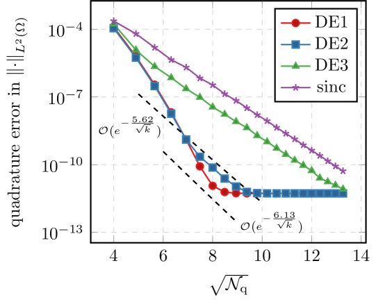
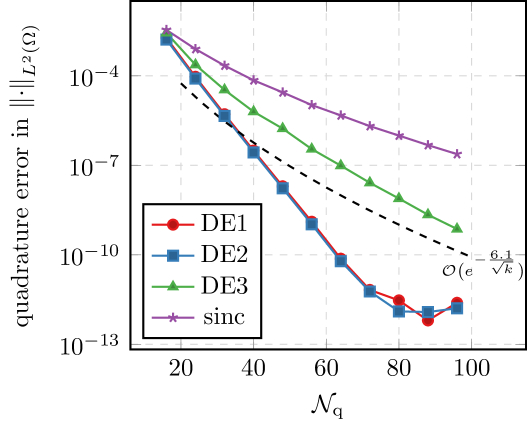
In this section, we focus on a scalar quadrature problem. Namely, we investigate how well our quadrature scheme can approximately evaluate the following functions using the Riesz-Dunford calculus (a) $z^{-\beta}$ and (b) $e_{\alpha,1}(-t^{\alpha}z^{\beta})$ at different values $\lambda\in(4,\infty)$ . This is equivalent to solving the elliptic and parabolic problem with data consisting of a single eigenfunction corresponding to the eigenvalue $\lambda$ . Throughout, we used $\kappa:=3$ . Theoretical investigations revealed, that the quadrature error is largest at $\ln(\lambda)\sim k^{-1/2}$ (see the proof of Corollary 3.5). Therefore, we make sure that for each $k$ under consideration, such a value of $e^{\frac{1}{\sqrt{k}}}$ is among the $\lambda$ -values sampled. More precisely, the sample points consist of

\displaystyle\bigcup_{\mathcal{N}_{\textrm{q}}=1}^{N_{\max}}\big{\{}5+\exp\big{(}2\sqrt{\beta/k(\mathcal{N}_{\textrm{q}})}\big{)}\big{\}}\cup\big{\{}5+\exp(\beta/k(\mathcal{N}_{\textrm{q}}))\big{\}}\qquad\text{with }\qquad k(\mathcal{N}_{\textrm{q}})=0.9\ln(\mathcal{N}_{\textrm{q}})/\mathcal{N}_{\textrm{q}},

and we consider the maximum error over all these samples. We used $t:=1$ for all experiments.

Refer to caption — (a) $f(z)=z^{-0.6}$ .

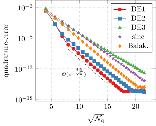
We observe that for the most part, choosing $\sigma=1/2$ and $\theta$ moderately large gives the best result. This agrees with our theoretical findings. This method fails to converge though if $\alpha=\beta=1$ is chosen as the parameters for the Mittag-Leffler function. This also agrees with the theory, because in this case, $\psi_{\sigma,\theta}$ fails to map into the domain where $e_{\alpha,\mu}$ is decaying (see (4.7)). This shows that the restriction on $\sigma$ in the theorems of Section 4 is necessary. If we only consider the elliptic problem, no such restriction is necessary, as the decay property is valid on all of the complex plane. All the other methods perform well in all of the cases. The straight-forward double exponential formula, i.e. $\sigma=\theta=1$ , is often outperformed by the simple sinc quadrature scheme, (except in the $\alpha=\beta=1$ case of the exponential). For comparison, we’ve included the (rounded) predicted rate for the DE1 scheme in the plots. We observe that for several applications our estimates appear sharp. For $f(z)=z^{-1}$ the scheme outperforms the prediction, but this might be due to a large preasymptotic regime. We note that for $e^{-z^{\beta}}$ , we expect better estimates than the ones presented in this article to be possible due to the exponential decay. This is also true for the standard sinc methods, see [BLP17a].

Second, we look at the case of a single frequency $\lambda$ and see how the convergence rate decays as $\lambda\to\infty$ . In order to better see the $\lambda$ -dependence of the quadrature error, we consider the relative error of the quadrature, i.e., we look at $E^{\lambda}(z^{-\beta})/\lambda^{-\beta}$ for $\beta=0.5$ . The theory from Theorem 3.4 predicts behavior of the form $e^{-\frac{\gamma}{\ln(\lambda)k}}$ , i.e., the rate drops like $\ln(\lambda)$ . In Figure 5.2, we can see this behavior quite well. In comparison, using standard $\operatorname{sinc}$ quadrature gives a $\lambda$ -robust asymptotic rate, but only of order $\sqrt{\mathcal{N}_{\textrm{q}}}$ .


5.2

Figure 5.2: Comparison of

\lambda

dependence for different quadrature schemes

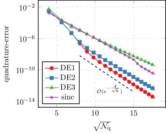
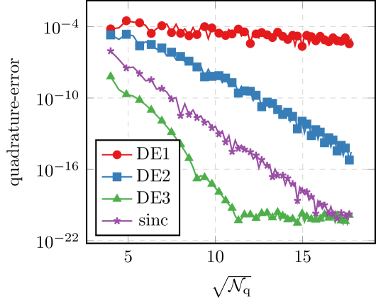
5.2 A 2d example

In order to confirm our theoretical findings in a more complex setting, we now look at a 2d model problem with more realistic data than a single eigenfunction. Namely we consider the unit square $\Omega=(0,1)^{2}$ . We focus on two cases: first we look at what happens if the initial condition does not satisfy any compatibility condition, i.e., $u_{0}\notin\mathbb{H}^{2\rho}(\Omega)$ for $\rho\geq 1/4$ . The second example is then taken such that the data is (almost) in the Gevrey-type class as required by Corollary 3.9 and Theorem 4.7. The inhomogenity in time is taken as $f(t):=\sin(t)u_{0}$ , thus possessing analogous regularity properties. We computed the function at $t=0.1$ .

For the discretization in space and of the convolution in time of (4.2), we consider the scheme presented in [MR21]. It is based on $hp$ -finite elements for the Galerkin solver and a $hp$ -quadrature on a geometric grid in time for the convolution. As it is shown there, such a scheme delivers exponential convergence with respect to the polynomial degree and the number of quadrature points. Since we are not interested in these kinds of discretization errors, we fixed these discretization parameters in order to give good accuracy and only focus on the error due to discretizing the functional calculus.

Since the exact solution is not available, we computed a reference solution with high accuracy and compared our other approximations to it. The reference solution is computed by the DE1 scheme (as it outperformed the others) by using 8 additional quadrature points to the finest approximation present in the graph. As the DE1 scheme has finished convergence at this point, we can expect this to be a good approximation.

We start with the parabolic problem. The initial condition is given by

u_{0}(x,y):=\omega^{-1}\exp\Big{(}-\frac{(x-0.5)^{2}}{\omega}\Big{)}\exp\Big{(}-\frac{(y-0.5)^{2}}{\omega}\Big{)}.

For $\omega:=1$ , this function does not vanish near the boundary of $\Omega$ and therefore only satisfies $u_{0}\in\mathbb{H}^{1/2-\varepsilon}(\Omega)$ . We are in the setting of Lemma 4.4. By inserting $\rho=1/4$ (up to $\varepsilon$ ) and $r=0$ , the predicted rates for DE1 and DE2 are roughly $e^{-\frac{6.13}{\sqrt{k}}}$ and $e^{-\frac{5.62}{k}}$ respectively. Figure 3(a) contains our findings. We observe that all methods converge with exponential rate proportional to $\sqrt{\mathcal{N}_{\textrm{q}}}$ . The double exponential formulas outperforming the standard $\operatorname{sinc}$ quadrature. We also observe that picking $\sigma\neq 1$ and $\theta\neq 1$ can greatly improve the convergence. The best results being delivered by DE1, i.e. $\sigma=1/2$ and $\theta=4$ . For DE1 and DE2, we observe that for a large part of the computation, the scheme outperforms the predicted asymptotic rate, but for DE2, the rate appears sharp for large values of $\mathcal{N}_{\textrm{q}}$ .

As a second example, we used $\omega=0.01$ . This function is almost equal to $0$ in a vicinity of the boundary of $\Omega$ . Thus we may hope to achieve the improved convergence rate of Theorem 4.7. Figure 3(b) shows that it is plausible that the exponential rate of order $\mathcal{N}_{\textrm{q}}$ is achieved, although the difference is hard to make out. What can be said is that all the double exponential schemes greatly outperform the standard $\operatorname{sinc}$ quadrature. The best results are again achieved by DE1, which also greatly outperforms the predicted rate for the non-smooth case.

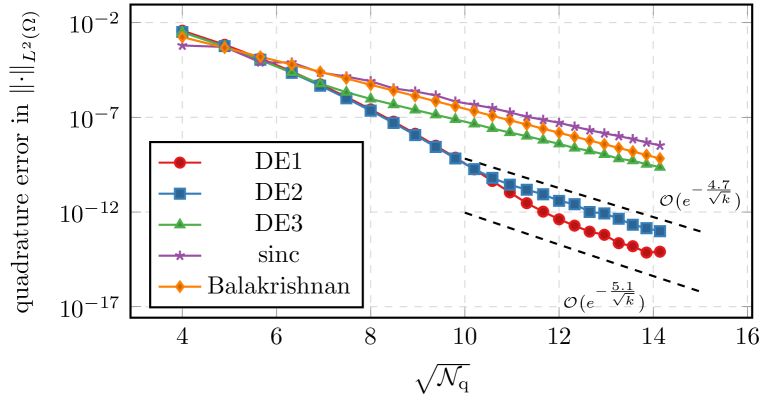
We also looked at the convergence for the elliptic problem. In this class, we also included the method based on the Balakrishnan formula. As a model problem we again used the unit square. We chose $f=1$ as the constant function and $\beta:=0.4$ . We again observe that with $\theta=4$ and $\sigma\in\{0.5,1\}$ , the double exponential formulas significantly outperform the standard $\operatorname{sinc}$ based strategies, where $\sigma=0.5$ again delivers the best performance. The predicted rates for DE1 and DE2 in this case are $e^{-\frac{4.7}{\sqrt{k}}}$ and $e^{-\frac{5.1}{\sqrt{k}}}$ respectively. We observe that asymptotically our estimates appear sharp, but with a large range of values, for which the scheme outperforms the predictions.

References

[AB17a] G. Acosta and J. P. Borthagaray. A fractional Laplace equation: regularity of solutions and finite element approximations. SIAM J. Numer. Anal., 55(2):472–495, 2017.
[AB17b] H. Antil and S. Bartels. Spectral approximation of fractional PDEs in image processing and phase field modeling. Comput. Methods Appl. Math., 17(4):661–678, 2017.
[ABH19] G. Acosta, J. P. Borthagaray, and N. Heuer. Finite element approximations of the nonhomogeneous fractional Dirichlet problem. IMA J. Numer. Anal., 39(3):1471–1501, 2019.
[BBN⁺18] A. Bonito, J. P. Borthagaray, R. H. Nochetto, E. Otárola, and A. J. Salgado. Numerical methods for fractional diffusion. Comput. Vis. Sci., 19(5-6):19–46, 2018.
[BLP17a] A. Bonito, W. Lei, and J. E. Pasciak. The approximation of parabolic equations involving fractional powers of elliptic operators. J. Comput. Appl. Math., 315:32–48, 2017.
[BLP17b] A. Bonito, W. Lei, and J. E. Pasciak. Numerical Approximation of Space-Time Fractional Parabolic Equations. Comput. Methods Appl. Math., 17(4):679–705, 2017.
[BLP19] A. Bonito, W. Lei, and J. E. Pasciak. On sinc quadrature approximations of fractional powers of regularly accretive operators. J. Numer. Math., 27(2):57–68, 2019.
[BMN⁺18] L. Banjai, J. M. Melenk, R. H. Nochetto, E. Otárola, A. J. Salgado, and C. Schwab. Tensor FEM for Spectral Fractional Diffusion. Foundations of Computational Mathematics, Oct 2018.
[BP15] A. Bonito and J. E. Pasciak. Numerical approximation of fractional powers of elliptic operators. Math. Comp., 84(295):2083–2110, 2015.
[BV16] C. Bucur and E. Valdinoci. Nonlocal diffusion and applications, volume 20 of Lecture Notes of the Unione Matematica Italiana. Springer, [Cham]; Unione Matematica Italiana, Bologna, 2016.
[EMOT81] A. Erdélyi, W. Magnus, F. Oberhettinger, and F. G. Tricomi. Higher transcendental functions. Vol. III. Robert E. Krieger Publishing Co., Inc., Melbourne, Fla., 1981. Based on notes left by Harry Bateman, Reprint of the 1955 original.
[GH15] P. Gatto and J. S. Hesthaven. Numerical approximation of the fractional laplacian via $hp$ -finite elements, with an application to image denoising. Journal of Scientific Computing, 65(1):249–270, Oct 2015.
[GO08] G. Gilboa and S. Osher. Nonlocal operators with applications to image processing. Multiscale Model. Simul., 7(3):1005–1028, 2008.
[KR19] B. Kaltenbacher and W. Rundell. Regularization of a backward parabolic equation by fractional operators. Inverse Probl. Imaging, 13(2):401–430, 2019.
[KST06] A. A. Kilbas, H. M. Srivastava, and J. J. Trujillo. Theory and applications of fractional differential equations, volume 204 of North-Holland Mathematics Studies. Elsevier Science B.V., Amsterdam, 2006.
[LB92] J. Lund and K. L. Bowers. Sinc methods for quadrature and differential equations. Society for Industrial and Applied Mathematics (SIAM), Philadelphia, PA, 1992.
[LPGea20] A. Lischke, G. Pang, M. Gulian, and et al. What is the fractional Laplacian? A comparative review with new results. J. Comput. Phys., 404:109009, 62, 2020.
[MMR20] J. Markus Melenk and A. Rieder. hp-FEM for the fractional heat equation. IMA Journal of Numerical Analysis, 04 2020. drz054.
[Mor91] M. Mori. Developments in the double exponential formulas for numerical integration. In Proceedings of the International Congress of Mathematicians, Vol. I, II (Kyoto, 1990), pages 1585–1594. Math. Soc. Japan, Tokyo, 1991.
[MPSV18] D. Meidner, J. Pfefferer, K. Schürholz, and B. Vexler. $hp$ -finite elements for fractional diffusion, 2018.
[MR21] J. M. Melenk and A. Rieder. An exponentially convergent discretization for space-time fractional parabolic equations using $hp$ -fem. in preparation, 2021.
[NOS15a] R. H. Nochetto, E. Otárola, and A. J. Salgado. A PDE approach to fractional diffusion in general domains: a priori error analysis. Found. Comput. Math., 15(3):733–791, 2015.
[NOS15b] R. H. Nochetto, E. Otárola, and A. J. Salgado. A PDE approach to fractional diffusion in general domains: a priori error analysis. Found. Comput. Math., 15(3):733–791, 2015.
[NOS16] R. H. Nochetto, E. Otárola, and A. J. Salgado. A PDE approach to space-time fractional parabolic problems. SIAM J. Numer. Anal., 54(2):848–873, 2016.
[Rod93] L. Rodino. Linear partial differential operators in Gevrey spaces. World Scientific Publishing Co., Inc., River Edge, NJ, 1993.
[Ste93] F. Stenger. Numerical methods based on sinc and analytic functions, volume 20 of Springer Series in Computational Mathematics. Springer-Verlag, New York, 1993.
[SZB⁺18] H. Sun, Y. Zhang, D. Baleanu, W. Chen, and Y. Chen. A new collection of real world applications of fractional calculus in science and engineering. Communications in Nonlinear Science and Numerical Simulation, 64:213 – 231, 2018.
[TM74] H. Takahasi and M. Mori. Double exponential formulas for numerical integration. Publ. Res. Inst. Math. Sci., 9:721–741, 1973/74.
[V1́7] J. L. Vázquez. The mathematical theories of diffusion: nonlinear and fractional diffusion. In Nonlocal and nonlinear diffusions and interactions: new methods and directions, volume 2186 of Lecture Notes in Math., pages 205–278. Springer, Cham, 2017.

Appendix A Properties of the coordinate transform $\psi_{\sigma,\theta}$

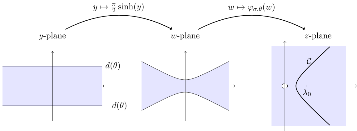
In this appendix, we study the transformation $\psi_{\sigma,\theta}$ in detail, as it is crucial to understand the double exponential quadrature scheme. Since this transformation is itself defined in a two-part way, we introduce the following nomenclature.

Definition A.1.

We call the complex plane on which $\psi_{\sigma,\theta}$ is defined the $y$ -plane, mainly using the parameter $y$ for its points. The main subset of interest there is the strip $D_{d(\theta)}$ .

Using the function $y\mapsto\frac{\pi}{2}\sinh(y)$ , the $y$ -plane is mapped to the $w$ -plane. The most interesting set is the image of $D_{d(\theta)}$ under this deformation, denoted by $H_{\theta}:=\big{\{}\frac{\pi}{2}\sinh(y),y\in D_{d(\theta)}\big{\}}$ (named due to its hyperbola shape).

Finally, using the function $\varphi_{\sigma,\theta}(w):=\kappa[\cosh(\sigma w)+i\theta\sinh(w)]$ , mapping $H_{\theta}\to\mathbb{C}$ , we arrive at the $z$ -plane which corresponds to the range of $\psi_{\sigma,\theta}$ , and the domain of the functions used for the Riesz-Dunford calculus. The situation is summarized in Figure A.1.

If we talk about generic complex numbers without relation to any of the specific planes, we use the letter $\zeta$ instead.

We start out with some basic properties of $\sinh$ .

Lemma A.2.

The map $y\mapsto\frac{\pi}{2}\sinh(y)$ has the following properties:

(i)

It is a bijective mapping $D_{d(\theta)}\to H_{\theta}$ , see Figure A.1.
(ii)

For $\left|\operatorname{Re}(\zeta)\right|\geq\zeta_{0}>0$ , there exist constants $c_{1},c_{2}>0$ depending only on $\zeta_{0}$ such that

$c_{1}\left|\sinh(\zeta)\right|\leq\left|\cosh(\zeta)\right|\leq c_{2}\left|\sinh(\zeta)\right|.$
(iii)

For any $\delta<\pi/2$ , $\sinh$ maps the domain $D^{\mathrm{exp}}_{\delta}$ , as defined in (2.2), to a strip of size $\delta$ , i.e.,

$\displaystyle\left|\operatorname{Im}(\sinh(y))\right|\leq\delta\qquad\forall y\in D^{\mathrm{exp}}_{\delta}.$ (A.1)

Proof.

Ad (i): It is well known that $\sinh$ is injective for $\left|\operatorname{Im}(y)\right|<\pi/2$ . Since $H_{\theta}$ is defined as the range of the map this is sufficient. Part (ii) is an easy consequence of the fact that $\sinh$ and $\cosh$ have the same asymptotic behavior for $\operatorname{Re}(\zeta)\to\infty$ . To see (iii), we estimate for $y\in D^{\mathrm{exp}}_{\delta}$ :

\displaystyle\left|\operatorname{Im}(\sinh(y))\right|

\displaystyle=\cosh(\operatorname{Re}(y))\left|\sin(\operatorname{Im}(y))\right|\leq\delta\,\cosh(\operatorname{Re}(y))e^{-\left|\operatorname{Re}(y)\right|}\leq\delta.\qed

Lemma A.3.

$\psi_{\sigma,\theta}$ is analytic on the infinite strip $D_{d(\theta)}$ . For $d(\theta)$ sufficiently small, both $\psi_{\sigma,\theta}$ and $\psi_{\sigma,\theta}^{\prime}$ are non-vanishing on $D_{d(\theta)}$ .

Proof.

The analyticity of $\psi_{\sigma,\theta}$ is clear. In order to analyze the roots, we first rewrite for $w=a+ib$ , separating the real and imaginary parts:

	$\displaystyle\cosh(\sigma w)+i\theta\sinh(w)$	$\displaystyle=\Big{(}\cosh(\sigma a)\cos(\sigma b)-\theta\cosh(a)\sin(b)\Big{)}$		(A.2)
		$\displaystyle+i\Big{(}\sinh(\sigma a)\sin(\sigma b)+\theta\sinh(a)\cos(b)\Big{)}.$		(A.2)

We first focus on the case $\mathbf{\boldsymbol{\sigma}=1}$ . In this case, (A.2) shows that any root $y$ of $\psi_{\sigma,\theta}$ must satisfy for $w:=\frac{\pi}{2}\sinh(y)=:a+bi$ :

\displaystyle\cosh(a)\Big{(}\cos(b)-\theta\sin(b)\Big{)}

\displaystyle=0\quad\text{ and }\quad\sinh(a)\Big{(}\theta\cos(b)+\sin(b)\Big{)}=0.

Since $\cosh$ has no roots, we get $\cos(b)=\theta\sin(b)$ . As $\cos(b)=\theta\sin(b)$ and $\theta\cos(b)=-\sin(b)$ is impossible at the same time, we get that $a=0$ and $b=\tan^{-1}(1/\theta)+\ell\pi$ for some $\ell\in\mathbb{Z}$ .

It remains to show that $\frac{\pi}{2}\sinh(y)$ does not map to these points. Looking at the real part of $\sinh(y)$ we immediately deduce that if $\operatorname{Im}(y)\in(-\pi/2,\pi/2)$ , in order to produce a purely imaginary result, it must hold that $\operatorname{Re}(y)=0$ . For the imaginary part, we then get the equation:

\sin(\operatorname{Im}(y))=2\ell+\frac{2\tan^{-1}(1/\theta)}{\pi}\quad\text{for some $\ell\in\mathbb{Z}$}

which is not possible for $\left|\operatorname{Im}(y)\right|\leq d(\theta)<\sin^{-1}(\frac{2\tan^{-1}(1/\theta)}{\pi})$ . Next, we show that $\psi_{\sigma,\theta}^{\prime}$ also does not vanish. A simple calculation shows

\displaystyle\psi_{1,\theta}^{\prime}(y)=i\theta\,\psi_{1,\frac{1}{\theta}}(-y)\frac{\pi}{2}\cosh(y).

(A.3)

Since the restriction $\theta\geq 1$ was not crucial for the proof, $\psi_{1,\frac{1}{\theta}}$ and $\cosh$ have no roots in the symmetric (w.r.t. sign flip) domain $D_{d(\theta)}$ . This shows that $\psi_{1,\theta}^{\prime}$ also is non-vanishing.

The case $\mathbf{\boldsymbol{\sigma}=1/2}$ is similar, but a little more involved. We first show that all zeros of $\cosh(\sigma w)+i\theta\sinh(w)$ satisfy $\operatorname{Re}(w)=0$ and $\left|\operatorname{Im}(w)\right|>w_{0}>0$ for a constant $w_{0}$ depending only on $\theta$ . If $\cosh(w/2)\neq 0$ we can use the double angle formula for $\sinh$ to get

\displaystyle 0=\cosh(w/2)\big{(}1+2\theta i\sinh(w/2)\big{)}\qquad\text{ which implies }\qquad\sinh(w/2)=\frac{i}{2\theta}.

Splitting into real and imaginary part, we get for $w=a+ib$ :

\displaystyle\sinh(a/2)\cos(b/2)=0\qquad\text{and }\qquad\cosh(a/2)\sin(b/2)=\frac{1}{2\theta}.

If $a\neq 0$ , we get that $\cos(b/2)=0$ and thus $\sin(b/2)=\pm 1$ . This would imply that $\left|\cosh(a/2)\right|=\frac{1}{2\theta}<1/2$ which is a contradiction. If $a=0$ , we get that

\left|b\right|\geq 2\big{|}{\sin^{-1}\Big{(}\frac{1}{2\theta}\Big{)}}\big{|}>0.

Similarly, one can argue if $\cosh(w/2)=0$ , that $a=0$ and $b=\pi(2\ell+1)$ . We then proceed just like in the case $\sigma=1$ to conclude that $\frac{\pi}{2}\sinh$ does not map to such points.

In order to investigate its roots, we compute the derivative of $\psi_{\frac{1}{2},\theta}$ as

\displaystyle\psi_{\frac{1}{2},\theta}^{\prime}(y)

\displaystyle=\Big{(}\frac{1}{2}\sinh\big{(}\pi\sinh(y)/4\big{)}+i\theta\cosh\big{(}\pi\sinh(y)/2\big{)}\Big{)}\frac{\pi}{2}\cosh(y).

(A.4)

Our main concern is when the first bracket reaches zero. Substituting $t:=\sinh(\pi\sinh(y)/4)$ and using the double angle formula for $\cosh$ we get

\displaystyle 0

\displaystyle=\frac{t}{2}+i\theta(1+2t^{2}).

Solving this equation, we get that $t$ is purely imaginary and for $\theta\geq 1$ satisfies $0<\left|\operatorname{Im}(t)\right|<1$ . Again writing $w=:a+ib$ we get

\displaystyle\sinh(a/2)\cos(b/2)=0\qquad\text{and }\qquad\cosh(a/2)\sin(b/2)=\operatorname{Im}(t).

Just like we did when showing $\psi_{\frac{1}{2},\theta}\neq 0$ we can argue that $a=0$ . We get $\sin(b/2)=\operatorname{Im}(t)$ . Since $t$ only depends on $\theta$ , we get that $\left|b\right|>b_{0}>0$ with a constant only depending on $\theta$ . We proceed as when showing $\psi_{\frac{1}{2},\theta}\neq 0$ to conclude that $\psi_{\frac{1}{2},\theta}^{\prime}$ has no root in $D_{d(\theta)}$ for $d$ sufficiently small (depending on $\theta$ ). ∎

Next, we study the growth of $\psi_{\sigma,\theta}(y)$ as $\left|\operatorname{Re}(y)\right|\to\infty$ .

Lemma A.4.

There exist constants $c_{1},c_{2}$ , $\gamma_{1},\gamma_{2}>0$ such that for $y\in D_{d(\theta)}$ we can estimate

\displaystyle c_{1}\exp(\gamma_{1}e^{\left|\operatorname{Re}(y)\right|})\leq\left|\psi_{\sigma,\theta}(y)\right|\leq c_{2}\exp(\gamma_{2}e^{\left|\operatorname{Re}(y)\right|}),

(A.5)

i.e., the growth of $\psi$ is double exponential. Additionally, we can bound

\displaystyle|{\psi_{\sigma,\theta}^{\prime}}(y)|\lesssim|\psi_{\sigma,\theta}(y)|\cosh(\operatorname{Re}(y)).

(A.6)

Proof.

We start with the simple case $\boldsymbol{\sigma}\mathbf{=1}$ . And focus on what happens if $\left|\operatorname{Re}(y)\right|>y_{0}>0$ for a to be tweaked constant $y_{0}$ . The values with $0\leq\left|\operatorname{Re}(y)\right|\leq y_{0}$ can be covered by adjusting $c_{1}$ and $c_{2}$ , due to the compactness of the set $\{y\in D_{d(\theta)}:\left|\operatorname{Re}(y)\right|\leq y_{0}\}$ and the fact that $\left|\psi_{\sigma,\theta}(y)\right|>0$ by Lemma A.3. We first only consider the $y-w$ part of the transformation. We compute, since $\frac{1}{2}<\cos(t)\leq 1$ for $t\in(-1/2,1/2)$ :

\displaystyle\left|\operatorname{Re}(\sinh(y))\right|

\displaystyle=\left|\sinh(\operatorname{Re}(y))\right|\cos(\operatorname{Im}(y))\sim\left|\sinh(\operatorname{Re}(y))\right|\sim c_{1}e^{\left|\operatorname{Re}(y)\right|}.

Easy calculation shows that for $h_{1}(\eta):=\left|\cos(\eta)-\theta\sin(\eta)\right|$ and $h_{2}(\eta):=\left|\theta\cos(\eta)+\sin(\eta)\right|$ it holds that $[h_{1}(\eta)]^{2}+[h_{2}(\eta)]^{2}=1+\theta^{2}$ . Thus, for $w\in H_{\theta}$ with $\left|\operatorname{Re}(w)\right|\geq 1$ , we can calculate:

	$\displaystyle\left\|\cosh(w)+i\theta\sinh(w)\right\|^{2}$	$\displaystyle=\left\|\cosh(\operatorname{Re}(w))\right\|^{2}[h_{1}(\operatorname{Im}(w))]^{2}+\left\|\sinh(\operatorname{Re}(w))\right\|^{2}[h_{2}(\operatorname{Im}(w))]^{2}$		(A.7)
		$\displaystyle\gtrsim\min\big{(}\cosh(\operatorname{Re}(w)),\left\|\sinh(\operatorname{Re}(w))\right\|\big{)}^{2}(1+\theta^{2})\;\gtrsim\;e^{2\left\|\operatorname{Re}(w)\right\|}.$		(A.7)

Overall, we see the lower bound of (A.5). The upper bound is easily seen, as $\left|\sinh(y)\right|$ and $\left|\cosh(y)\right|$ both grow exponentially and the bound only depends on the real part of the argument. (A.6) follows from (A.3) and the asymptotics (A.7)and (A.5).

We now look at how to adapt the proof to the case $\boldsymbol{\sigma}\mathbf{=1/2}$ . If $\left|\operatorname{Re}(w)\right|\geq 4\ln(2)$ , we get

\left|\cosh(w/2)+i\theta\sinh(w)\right|\\ \geq\theta\left|\sinh(w)\right|-\left|\cosh(w/2)\right|\geq\frac{1}{2}\Big{(}e^{\left|\operatorname{Re}(w)\right|}-2-e^{\left|\operatorname{Re}(w)/2\right|}\Big{)}\geq\frac{1}{4}e^{\left|\operatorname{Re}(w)\right|}.

(A.8)

The argument for the $y-w$ -transformation stays the same. The upper bound also follows easily from the triangle inequality and the growth of $\sinh$ and $\cosh$ .

To see (A.6), we combine (A.4) with the asymptotic estimate (A.8) to get

\displaystyle|{\psi_{\sigma,\theta}^{\prime}}(y)|

\displaystyle\lesssim e^{\pi\left|\operatorname{Re}(\sinh(y))\right|/2}\cosh(\operatorname{Re}(y))\lesssim|\psi_{\sigma,\theta}(y)|\cosh(\operatorname{Re}(y)).\qed

While on the full strip $D_{d(\theta)}$ , the image of the transformation is difficult to study, the restriction to a certain subdomain is much better behaved.

Lemma A.5.

For $\sigma=1$ , there exists a constant $\delta>0$ , depending on $\theta$ , such that restricted to the domain $D^{\mathrm{exp}}_{\delta}$ , $\psi_{1,\theta}$ maps to a sector in the right-half plane,

S_{\omega}:=\big{\{}z\in\mathbb{C}:\left|\operatorname{Arg}(z)\right|\leq\omega\big{\}}\qquad\text{with}\quad\omega<\frac{\pi}{2}.

For $\sigma=1/2$ , and for all $\varepsilon>0$ , there exists a constant $\delta>0$ , depending on $\theta$ and $\varepsilon$ , such that restricted to the domain $D^{\mathrm{exp}}_{\delta}$ the transformation $\psi_{\frac{1}{2},\theta}$ maps to the sector $S_{\pi/2+\varepsilon}$ .

In both cases, there exist constants $c_{1},c_{2}>0$ such that $\psi_{\sigma,\theta}$ satisfies for all $\lambda>\lambda_{0}>\kappa:$

\displaystyle\left|\psi_{\sigma,\theta}(y)-\lambda\right|\geq c_{1}\quad\text{and}\quad\left|\psi_{\sigma,\theta}^{\prime}(y)(\psi_{\sigma,\theta}(y)-\lambda)^{-1}\right|\leq c_{2}\cosh(\operatorname{Re}(y))\qquad\forall y\in D^{\mathrm{exp}}_{\delta},

(A.9)

where $c_{1},c_{2}$ only depend on $\lambda_{0}$ and $\theta$ .

Proof.

By Lemma A.2(iii) it is sufficient to consider the mapping of $\varphi_{\sigma,\theta}$ restricted to small strips around the real axis. We start with the simpler case $\boldsymbol{\sigma}\mathbf{=1}$ . Going back to (A.2) and writing $w:=\frac{\pi}{2}\sinh(y)=:a+ib$ , we note that if $\left|b\right|$ is sufficiently small, we can guarantee that ${\cos(b)-\theta\sin(b)}>c>0$ for some constant $c>0$ depending on $\theta$ . We have

	$\displaystyle\operatorname{Re}(\varphi_{\sigma,\theta}(w))$	$\displaystyle=\kappa\cosh(a)\big{(}\cos(b)-\theta\sin(b)\Big{)}>c\,\kappa\cosh(a),$
	$\displaystyle\left\|\operatorname{Im}(\varphi_{\sigma,\theta}(w))\right\|$	$\displaystyle=\kappa\left\|\sinh(a)\right\|\|\theta\cos(b)+\sin(b)\|\leq(1+\theta)\kappa\left\|\sinh(a)\right\|.$

Which easily gives

0\leq\frac{\left|\operatorname{Im}(\varphi_{\sigma,\theta}(w))\right|}{\operatorname{Re}(\varphi_{\sigma,\theta}(w))}\leq(1+\theta)c^{-1}\qquad\forall w\in\mathbb{C},\;\left|\operatorname{Im}(w)\right|\text{sufficiently small}.

Next, we show that for $\boldsymbol{\sigma=1/2}$ , sufficiently thin strips in the $w$ -domain are mapped to sectors with opening angle $\pi/2+\varepsilon$ . Such sectors are characterized by

-\operatorname{Re}(\varphi_{\sigma,\theta}(w))\leq\widetilde{\varepsilon}\left|\operatorname{Im}(\varphi_{\sigma,\theta}(w))\right|\qquad\forall\left|\operatorname{Im}(w)\right|<b_{0}(\widetilde{\varepsilon})

for $\widetilde{\varepsilon}>0$ depending on $\varepsilon$ . The interesting case is $\operatorname{Re}(\varphi_{\sigma,\theta}(w))<0$ . There, we get for $\left|b\right|\leq\pi$ :

\displaystyle-{\operatorname{Re}(\varphi_{\sigma,\theta}(w))}

\displaystyle=-\kappa\cosh(a/2)\cos(b/2)+\kappa\theta\cosh(a)\sin(b)\leq\kappa\theta\cosh(a)\left|\sin(b)\right|.

For the imaginary part, the double angle-formula gives:

	$\displaystyle\left\|\operatorname{Im}(\varphi_{\sigma,\theta}(w))\right\|$	$\displaystyle\geq\kappa\theta\left\|\sinh(a)\cos(b)\right\|-\kappa\left\|\sinh(a/2)\sin(b/2)\right\|$
		$\displaystyle\geq\frac{\kappa\theta}{2}\left\|\sinh(a)\cos(b)\right\|+\kappa\left\|\sinh(a/2)\right\|\big{(}\theta\cosh(a/2)\left\|\cos(b)\right\|-\left\|\sin(b/2)\right\|\big{)}.$

For $\left|b\right|$ sufficiently small, we get $\theta\cos(b)-\left|\sin(b/2)\right|>0$ , and thus the last term is non-negative. We conclude

\displaystyle-{\operatorname{Re}(\varphi_{\sigma,\theta}(w))}

\displaystyle\leq 2\left|\frac{\cosh(a)}{\sinh(a)}\frac{\sin(b)}{\cos(b)}\right|\left|\operatorname{Im}(\varphi_{\sigma,\theta}(w))\right|.

For $a>1$ , the first term is uniformly bounded. By making $b$ sufficiently small, we can ensure $\left|\sin(b)\right|/{\cos{b}}<\widetilde{\varepsilon}$ . For $a<1$ , we note that by restricting the values of $b$ it can be easily seen that $\operatorname{Re}(\varphi_{\sigma,\theta}(w))\geq 0$ . Thus we can conclude that $\psi_{\sigma,\theta}$ maps to the stated sectors.

Next, we prove the bounds on the distance to the real axis, again primarily investigating the behavior of $\varphi_{\sigma,\theta}$ in thin strips. We focus on $\boldsymbol{\sigma=1/2}$ . Since $\varphi_{\sigma,\theta}(0)=\kappa<\lambda_{0}$ and $\varphi_{\sigma,\theta}$ is continuous, there exist constants $0<q<1$ and $\widetilde{\delta}>0$ such that $\left|\varphi_{\sigma,\theta}(w)\right|<q\lambda_{0}$ for all $\left|w\right|<\widetilde{\delta}$ . This gives

\left|\varphi_{\sigma,\theta}(w)-\lambda\right|\geq\lambda-\left|\varphi_{\sigma,\theta}(w)\right|\geq\lambda_{0}-\left|\varphi_{\sigma,\theta}(w)\right|>(1-q)\lambda_{0}\qquad\forall\left|w\right|\leq\widetilde{\delta}.

By selecting $\delta<\widetilde{\delta}/2$ in the definition of $D^{\mathrm{exp}}_{\delta}$ , we may then continue by only considering $\left|a\right|:=\left|\operatorname{Re}(w)\right|>\widetilde{\delta}/2$ . The imaginary part of $\varphi_{\frac{1}{2},\theta}(y)$ satisfies:

	$\displaystyle\operatorname{Im}(\varphi_{\frac{1}{2},\theta}(y))$	$\displaystyle=\kappa\sinh(a/2)\sin(b/2)+\kappa\theta\sinh(a)\cos(b)$
		$\displaystyle=\kappa\sinh(a/2)\Big{(}\sin(b/2)+2\theta\cosh(a/2)\cos(b)\Big{)}.$

For $\left|b\right|\leq\pi/4$ we have $\sin(b/2)+2\cos(b)>0$ and thus can conclude that $|{\operatorname{Im}(\varphi_{\frac{1}{2},\theta}(y))}|\geq c>0$ and in turn $|{\varphi_{\frac{1}{2},\theta}(y)-\lambda}|\geq c>0$ . The case $\sigma=1$ follows similarly, but not using the double angle formula.

To see that $\psi_{\sigma,\theta}^{\prime}(y)(\psi_{\sigma,\theta}(y)-\lambda)^{-1}$ can also be uniformly bounded, we only need to focus on large values of $y$ (and therefore $w$ ). Asymptotically, we estimate for $\left|b\right|<\pi/4$ :

\displaystyle\left|\operatorname{Im}(\psi_{\sigma,\theta}(y))\right|

\displaystyle\geq-\kappa\left|\sinh(\sigma a)\right|\left|\sin(\sigma b)\right|+\kappa\theta\left|\sinh(a)\cos(b)\right|\gtrsim\left|\sinh(a)\right|\!\!\stackrel{{\scriptstyle\text{\eqref{eq:growth_phi} or \eqref{eq:psi_growth_w}}}}{{\gtrsim}}\!\!\left|\psi_{\sigma,\theta}(y)\right|.

Using (A.6) then concludes the proof. ∎

In order to apply the double exponential formulas for the Riesz-Dunford calculus, it is important to understand where $\psi_{\sigma,\theta}(z)$ hits the real line. We start with the $w$ -domain.

Lemma A.6.

Fix $\lambda\geq\lambda_{0}>1$ . Then the following holds for every $w\in\mathbb{C}$ with $\operatorname{Re}(w)\neq 0$ and

\displaystyle\cosh(\sigma w)+i\theta\sinh(w)=\lambda:

(A.10)

(i)

There exist constants $c_{1},c_{2},c_{3}>0$ such that $w$ satisfies

\displaystyle\log(\lambda)-c_{1}\leq\left|\operatorname{Re}(w)\right|

\displaystyle\leq\log(\lambda)+c_{1}\quad\text{and}\quad\left|\operatorname{Im}(w)\right|\geq\begin{cases}\tan^{-1}(\theta)&\text{if }\sigma=1\\ \max\big{(}\frac{\pi}{2}-\frac{c_{2}}{\theta\sqrt{\lambda}},c_{3})&\text{if }\sigma=1/2\end{cases},

where $c_{1}$ depends on $\lambda_{0}$ and $\theta$ , $c_{2}$ depends on $\lambda_{0}$ , and $c_{3}$ depends on $\theta$ .

(ii)

Given $0<r<R$ , the number $N_{w}(\lambda,r,R)$ of points $w$ satisfying (A.10) with $r\leq\left|\operatorname{Im}(w)\right|\leq R$ is bounded uniformly in $\lambda$ by

$N_{w}(\lambda,r,R)\leq C\left|R-r\right|$

The constant $C$ depends only on $\theta$ .
(iii)

There exist at most four values $p_{1},\dots,p_{4}$ depending on $\lambda$ , $\theta$ , and $\sigma$ such that all points satisfying (A.10) can be written as

$\displaystyle w=p_{j}+\frac{2\ell}{\sigma}\pi i\qquad\text{ for some $\ell\in\mathbb{Z}$, $j\in\{1,4\}$.}$ (A.11)

If $w$ solves (A.10) then $-\overline{w}$ does as well.

Proof.

We start with the simpler case $\sigma=1$ . By separating the real and imaginary part as in (A.2), we can observe that the critical points $w=a+ib$ with $a\neq 0$ are located at

\displaystyle\cosh(a)

\displaystyle=\frac{\lambda}{\sqrt{1+\theta^{2}}},\qquad b=-\tan^{-1}(\theta)+2\ell\pi,\quad\ell\in\mathbb{Z}.

(A.12)

This implies that $\left|a\right|\sim\ln(\lambda)$ , and we also see that for each $\ell$ , there are two such points, one in each half-plane. All the statements follow easily. Note that in (iii) only two families are needed.

For the remainder of the proof we therefore focus on the case $\sigma=1/2$ . Ad (i): We start with the bound on the real part and write $w=a+ib$ . We note that if $\left|a\right|>\max\big{(}1,2\ln\big{(}\frac{8}{\theta}\big{)}\big{)}$ one can estimate using elementary considerations that $e^{\left|a\right|}/4\leq\left|\sinh(w)\right|$ and $e^{\left|a\right|/2}/\theta\leq e^{\left|a\right|}/8$ .

We then calculate:

\displaystyle\frac{e^{\left|a\right|}}{4}

\displaystyle\leq\left|\sinh(w)\right|=\frac{1}{\theta}{\left|\lambda-\cosh(w/2)\right|}\leq\frac{\lambda}{\theta}+\frac{e^{\frac{\left|a\right|}{2}}}{\theta}\leq\frac{\lambda}{\theta}+\frac{e^{\left|a\right|}}{8}.

From this, the statement readily follows. The other direction is shown similarly:

\displaystyle e^{a}

\displaystyle\geq\left|\sinh(w)\right|=\frac{1}{\theta}{\left|\lambda-\cosh(w/2)\right|}\geq\frac{\lambda}{\theta}-\frac{e^{\frac{\left|a\right|}{2}}}{\theta}\geq\frac{\lambda}{\theta}-\frac{e^{\left|a\right|}}{8}.

For $\left|a\right|\leq\max\big{(}1,2\ln\big{(}\frac{8}{\theta}\big{)}\big{)}$ , we use the bound $\left|\varphi_{\sigma,\theta}(w)\right|\lesssim e^{\left|a\right|}$ to see that $\ln(\lambda)$ must be uniformly bounded. The final bound on the real part of $w$ then follows for $c_{1}:=\max\big{(}\ln(8/\theta),\ln(9\theta/8),\widetilde{c}\big{)}$ , where $\widetilde{c}$ is used to compensate for the case of small $a$ .

Looking at the imaginary part of equation (A.10), we get from the double-angle formulas

	$\displaystyle 0$	$\displaystyle=\sinh(a/2)\sin(b/2)+\theta\sinh(a)\cos(b)$
		$\displaystyle=\sinh(a/2)\Big{(}\!\sin(b/2)+2\theta\cosh(a/2)\big{(}1-2\sin^{2}(b/2)\big{)}\!\Big{)}.$		(A.13)

Since we assume $a\neq 0$ , we get by substituting $\tau:=\sin(b/2)$

\displaystyle 0=\tau+2\theta\cosh(a/2)(1-2\tau^{2})\qquad\text{ or }\qquad\tau=\frac{1\pm\sqrt{1+32\theta^{2}\cosh^{2}(a/2)}}{8\theta\cosh(a/2)}.

(A.14)

From this, using the asymptotic behavior

\tau=\pm\frac{1}{\sqrt{2}}+\mathcal{O}\Big{(}\frac{1}{\theta\cosh(a/2)}\Big{)}\quad\text{ and }\quad\sin^{-1}\Big{(}\frac{1}{\sqrt{2}}+h\Big{)}=\frac{\pi}{4}+\mathcal{O}(h)

the statement follows for large $a$ , since $b=2\sin^{-1}(\tau)$ and $\cosh(a/2)\gtrsim\sqrt{\lambda}$ by (i). For small $a$ , we note that (A.14) shows that $\operatorname{Im}(w)\neq 0$ . By continuity, it must therefore hold that $\left|\operatorname{Im}(w)\right|>0$ uniformly.

Ad (ii) and (iii): We square the defining equation (A.10), getting

	$\displaystyle\lambda^{2}$	$\displaystyle=\cosh^{2}(w/2)+2i\theta\cosh(w/2)\sinh(w)-\theta^{2}\sinh^{2}(w)$
		$\displaystyle=\cosh^{2}(w/2)+4i\theta\cosh^{2}(w/2)\sinh(w/2)-4\theta^{2}\sinh^{2}(w/2)\cosh^{2}(w/2).$		(A.15)

Writing $\cosh^{2}(w/2)=1+\sinh^{2}(w/2)$ , we get that $t:=\sinh(w/2)$ solves the quartic equation

\displaystyle\lambda^{2}

\displaystyle=1+t^{2}+4i\theta(1+t^{2})t-4\theta^{2}t^{2}-4\theta^{2}t^{4}.

(A.16)

This means there can be at most 4 such values $t_{0},\dots t_{4}$ for any $\lambda$ and it must hold that

\displaystyle\sinh(w/2)

\displaystyle=t_{j}\quad\text{or }\quad w=w_{j}+4\pi\ell i

Here $w_{j}$ is the solution with $\operatorname{Re}(w_{j})>0$ and minimal value of $\left|\operatorname{Im}(w_{j})\right|$ . (iii) and (ii) follow. The fact that $-\overline{w_{j}}$ also solves (A.10) follows by conjugating both sides of the equation (A.16). ∎

Next, we show that points which have positive distance to the poles in the $w$ -plane are mapped to points with distance $\lambda$ in the $z$ -plane. Note that in the following Lemma we include some additional points in order to avoid distinguishing more cases. We also exclude most of the imaginary axis, as for small values of $\lambda$ it might contain poles which are structurally different than the ones involving large $\lambda$ .

Lemma A.7.

Define

b_{0}:=\max\big{\{}b\geq 0:\quad\left|\varphi_{\sigma,\theta}(i\tau)\right|\leq(\lambda_{0}+\kappa)/2\quad\forall\left|\tau\right|\leq b\big{\}}.

Fix $\lambda\geq\lambda_{0}>\kappa$ and define the set

\displaystyle\mathcal{M}_{\lambda}

\displaystyle:=\Big{\{}p_{\lambda}+i\ell\pi,\;\text{with }\;p_{\lambda}\in\mathbb{C}\text{ such that }\varphi_{\sigma,\theta}(p_{\lambda})=\lambda\text{ and }\ell\in\mathbb{Z}\Big{\}}\cup\{ib:\;\left|b\right|\leq b_{0}\}.

For any $\delta>0$ , there exists a constant $c(\delta)>0$ , depending only on $\delta$ and $\theta$ , such that for all $w\in\mathbb{C}$ with $\operatorname{dist}(w,\mathcal{M}_{\lambda})>\delta$ we can estimate

\left|\varphi_{\sigma,\theta}(w)-\lambda\right|\geq c(\delta)\lambda.

Proof.

We first deal with the issues close to the imaginary axis. Since $\left|\varphi_{\sigma,\theta}(ib)\right|\leq(\lambda_{0}+\kappa)/2$ if $\left|b\right|\leq b_{0}$ , we can find $\varepsilon\in(0,\delta/2)$ such that

\displaystyle\left|\varphi_{\sigma,\theta}(\widetilde{w})\right|<3\lambda_{0}/4+\kappa/4\quad\text{for all}\quad\widetilde{w}\in U_{\varepsilon}

\displaystyle:=\big{\{}\left|\operatorname{Re}(\widetilde{w})\right|\leq\varepsilon\;\text{and}\;\left|\operatorname{Im}(\widetilde{w})\right|\leq b_{0}\big{\}}.

If $\left|\operatorname{Re}(w)\right|\leq\varepsilon$ , the distance condition to $\mathcal{M}_{\lambda}$ implies $\left|\operatorname{Im}(w)\right|\leq b_{0}-\delta/2$ and thus $w\in U_{\varepsilon}$ . We can therefore calculate:

\displaystyle\left|\varphi_{\sigma,\theta}(w)-\lambda\right|\geq\lambda-\left|\varphi_{\sigma,\theta}(w)\right|\geq\frac{\lambda}{4}\Big{(}1-\frac{\kappa}{\lambda_{0}}\Big{)}.

Next, we deal with small values of $\lambda$ . For constants $\Lambda$ , $C_{w}$ to be fixed later, consider $\lambda\in[\lambda_{0},\Lambda]$ and define the set

\mathcal{R}:=\{w\in\mathbb{C}:\;\left|\operatorname{Re}(z)\right|\geq\varepsilon,\left|w\right|\leq C_{w}\}.

We show that the stated bound holds for $w\in\mathcal{R}$ . By the Lemma A.6(iii), the points of $\mathcal{M}_{\lambda}$ can be written as

\mathcal{M}_{\lambda}=\Big{\{}p_{j}+\pi\ell i,\;\;\ell\in\mathbb{Z},\;j=1,\dots,4\Big{\}}\cup\Big{\{}ib:\;\left|b\right|\leq b_{0}\Big{\}}

for some reference points $p_{j}\in\mathbb{C}$ , w.l.o.g. $\left|\operatorname{Im}(p_{j})\right|\leq\pi$ . We introduce set

\mathcal{M}_{\Lambda,C_{w}}:=\Big{\{}p_{j}+\ell\pi i,\;\left|\ell\right|\leq L,\,j=1,\dots,4\Big{\}}

where $L:=\lceil(C_{w}+1)/\pi\rceil$ is taken large enough that for all $\lambda\in[\lambda_{0},\Lambda]$ , it holds that

\mathcal{M}_{\lambda}\cap\mathcal{R}\subseteq\mathcal{M}_{\Lambda,C_{w}},

i.e., it contains all the poles of size less or equal than $C_{w}$ uniformly in $\lambda$ (but possibly also some larger ones). We consider the map

\Phi(\lambda,w):=\big{(}\varphi_{\sigma,\theta}(w)-\lambda\big{)}^{-1}\prod_{p_{\lambda}\in\mathcal{M}_{\Lambda,C_{w}}}{(w-p_{\lambda})}.

By the inverse function theorem, the points $p_{j}=\varphi_{\sigma,\theta}^{-1}(\lambda)$ depend continuously on $\lambda$ since $\varphi_{\sigma,\theta}^{\prime}\neq 0$ away from the imaginary axis (where we stay away from by construction). Thus, also the other points $p_{\lambda}$ depend continuously on $\lambda$ . Similarly, the denominator only has simple zeros for $w\in\mathcal{M}_{\lambda}$ . Since, in that case the numerator also vanishes one can argue that $\Phi$ has a continuous extension to $[\lambda_{0},\Lambda]\times\mathcal{R}$ which is bounded, i.e., it holds

\left|\frac{\prod_{p_{\lambda}\in\mathcal{M}_{\Lambda,C_{w}}}{(w-p_{\lambda})}}{\varphi_{\sigma,\theta}(w)-\lambda}\right|\leq C(\Lambda,C_{W})\qquad\text{or}\qquad\left|\varphi_{\sigma,\theta}(w)-\lambda\right|\geq\frac{1}{C(\Lambda,C_{W})}\prod_{p_{\lambda}\in\mathcal{M}_{\Lambda,C_{w}}}{\left|w-p_{\lambda}\right|}.

Thus, if $w$ is separated from $\mathcal{M}_{\lambda}$ and the imaginary axis, so is $\varphi_{\sigma,\theta}(w)$ from $\lambda$ . If $\lambda\in[0,\Lambda]$ and $\left|w\right|>C_{w}:=\max(\log(2\Lambda/c_{1}),4\ln(2))$ , (where $c_{1}$ is the constant in (A.7) or (A.8)) we get:

\left|\varphi_{\sigma,\theta}(w)-\lambda\right|\geq\left|\varphi_{\sigma,\theta}(w)\right|-\lambda\quad\;\stackrel{{\scriptstyle\mathclap{\eqref{eq:growth_phi},\eqref{eq:psi_growth_w}}}}{{\geq}}\quad\;c_{1}e^{\left|\operatorname{Re}(w)\right|}-\Lambda\geq\Lambda\geq\lambda.

We therefore may from now on assume that $\lambda$ is sufficiently large as we see fit. In preparation for the rest of the proof, we note that for $\zeta,\mu\in\mathbb{R}$ , w.l.o.g., $\left|\zeta\right|\leq\left|\mu\right|$ :

\displaystyle\left|\cosh(\mu)-\cosh(\zeta)\right|

\displaystyle=\cosh(\left|\mu\right|)-\cosh(\left|\zeta\right|)=\int_{\left|\zeta\right|}^{\left|\mu\right|}{\sinh(\tau)\,d\tau}\geq\sinh(\left|\zeta\right|)(\left|\mu\right|-\left|\zeta\right|).

(A.17)

Because it is much simpler, we start with the case $\boldsymbol{\sigma}\mathbf{=1}$ . We note that in this case $\mathcal{M}_{\lambda}$ consists of the points mapped to $\pm\lambda$ . We distinguish three cases, depending on whether $\operatorname{Re}(w)$ is small and if $\operatorname{Im}(w)$ is close to a pole or not.

Case 1:

$(1+\theta)\kappa\cosh(\operatorname{Re}(w))<\lambda/2:$ The triangle inequality gives:

\displaystyle\left|\kappa[\cosh(w)+i\theta\sinh(w)]-\lambda\right|

\displaystyle\geq\lambda-(1+\theta)\kappa\cosh(\operatorname{Re}(w))\geq\frac{\lambda}{2}.

Case 2:

$2(1+\theta)\kappa\cosh(\operatorname{Re}(w))\geq\lambda$ and there exists a point $p\in\mathcal{M}_{\lambda}$ with $\left|\operatorname{Im}{w}-\operatorname{Im}{p}\right|\leq\varepsilon_{1}$ for $\varepsilon_{1}$ sufficiently small. We note that this implies that $\left|\operatorname{Re}(w)-\operatorname{Re}(p)\right|$ is positive. Due to the symmetry in (A.11) we may in addition assume that $\operatorname{sign}(\operatorname{Re}(w))=\operatorname{sign}(\operatorname{Re}(p))$ . Writing $h(\eta):=\cos(\eta)-\theta\sin(\eta)$ , we note that $\left|h(\operatorname{Im}(w))\right|>c>0$ by (A.12) and the fact that adding $\pi\ell$ might only change the sign. If $h(\operatorname{Im}(p))\geq 0$ , we consider the real part of $\varphi_{\sigma,\theta}(w)-\lambda$ to get:

\left|\cosh(\operatorname{Re}(w))h(\operatorname{Im}(w)))-\lambda\right|\\ \begin{aligned} &=\left|\cosh(\operatorname{Re}(w))h(\operatorname{Im}(p))-\lambda+\cosh(\operatorname{Re}(w))\big{(}h(\operatorname{Im}(w))-h(\operatorname{Im}{p})\big{)}\right|\\ &\geq\left|\cosh(\operatorname{Re}(w))h(\operatorname{Im}{p})-\lambda\right|-\cosh(\operatorname{Re}(w))\left|h(\operatorname{Im}(w))-h(\operatorname{Im}{p})\right|\\ &\stackrel{{\scriptstyle\mathclap{\eqref{eq:difference_of_cosh}}}}{{\geq}}\min\big{(}\left|\sinh(\operatorname{Re}(w))\right|,\left|\sinh(\operatorname{Re}(p))\right|\big{)}\left|\operatorname{Re}(w)-\operatorname{Re}(p)\right|-2\cosh(\operatorname{Re}(w))\varepsilon_{1}\\ &\gtrsim\lambda\end{aligned}

where in the last step we chose $\varepsilon_{1}$ sufficiently small (but independent of $\lambda$ ). If $h(\operatorname{Im}(p))\leq 0$ , by continuity we can enforce $h(\operatorname{Im}(w))\leq 0$ as long as $\varepsilon_{1}$ is sufficiently small. The necessary calculation then is even easier because $\varphi_{\sigma,\theta}(w)$ maps to the left half-plane.

Case 3:

$2(1+\theta)\cosh(\operatorname{Re}(w))\geq\lambda$ and $\left|\operatorname{Im}(w)-\operatorname{Im}(p)\right|\geq\varepsilon_{1}>0$ for all $p\in\mathcal{M}_{\lambda}$ . We estimate imaginary part of $\varphi_{\sigma,\theta}$ . Since $\operatorname{Im}(w)$ has positive distance from the points in (A.12), we get $\left|\sin(\operatorname{Im}(w))+\theta\cos(\operatorname{Im}(w))\right|>c>0$ . Which in term gives

\left|\sinh(a)\right|\left|\sin(\operatorname{Im}(w))+\cos(\operatorname{Im}(w))\right|\geq c\left|\sinh(\operatorname{Re}(w))\right|\gtrsim\lambda

where the last part only holds for large enough cases of $\operatorname{Re}(w)$ not covered by Case 1.

Now we show, how the proof has to be adapted for the case $\boldsymbol{\sigma}\mathbf{=1/2}$ , again focusing on the asymptotic case of large $\lambda$ . By Lemma A.6(i), all the points $p\in\mathcal{M}_{\lambda}$ satisfy $\left|\operatorname{Re}(p)\right|\sim\log(\lambda)$ . Looking at the imaginary part of the defining equation for $p$ we get that

\displaystyle\left|\cos(\operatorname{Im}(p))\right|

\displaystyle=\left|\frac{\sinh(\operatorname{Re}(p)/2)}{\theta\cosh(\operatorname{Re}(p))}\sin(\operatorname{Re}(p))\right|\lesssim\frac{e^{-a/2}}{\theta}\lesssim\lambda^{-1/2}.

Thus, for any $\varepsilon_{2}>0$ , assuming $\lambda$ is sufficiently large, all the points $p\in\mathcal{M}_{\lambda}$ satisfy $\cos(p)<\varepsilon_{2}$ .

We again have to distinguish three cases:

Case 1:

$(1+\theta)\cosh(\operatorname{Re}(w))<\lambda/2:$ One can argue just like in the $\sigma=1$ case.

Case 2:

$2(1+\theta)\cosh(\operatorname{Re}(w))\geq\lambda$ and there exists a point $p\in\mathcal{M}_{\lambda}$ with $\left|\operatorname{Im}{w}-\operatorname{Im}{p}\right|\leq\varepsilon_{1}$ for $\varepsilon_{1}$ sufficiently small. We note that this implies that $\left|\operatorname{Re}(w)-\operatorname{Re}(p)\right|$ is positive. Since $\left|\cos(w)\right|<\varepsilon_{2}$ , we note that $\left|\sin(w)\right|>1-\varepsilon_{2}$ . By possibly adding $i\ell\pi$ , we can write

\displaystyle\lambda=-\theta\cosh(\operatorname{Re}(p))\sin(\operatorname{Im}(p+\ell i\pi))+\cosh(\operatorname{Re}(p/2))\sin(\operatorname{Im}(p+\ell i\pi)/2).

(A.18)

For large values of $\lambda$ , the $\cosh(\operatorname{Re}(p))$ term is dominating. Therefore, we have $\operatorname{sign}(\operatorname{Re}(\varphi_{\sigma,\theta}(p)))=-\operatorname{sign}(\sin(\operatorname{Im}(p)))$ . By continuity we can enforce that $\operatorname{sign}(\sin(\operatorname{Im}(w)))=\operatorname{sign}(\sin(\operatorname{Im}(p)))$ . Since for the case $\operatorname{Re}(\varphi_{\sigma,\theta}(w))\leq 0$ the statement is trivial, we only have to consider the case $\operatorname{sign}(\sin(\operatorname{Im}(w)))=-1$ or $\ell=0$ in (A.18). We look at the real part of $\varphi_{\sigma,\theta}(w)-\lambda$ to get:

	$\displaystyle\big{\|}-\theta\cosh($	$\displaystyle\operatorname{Re}(w))\sin(\operatorname{Im}(w))-\lambda+\cosh(\operatorname{Re}(w)/2)\cos(\operatorname{Im}(w)/2)\big{\|}$
		$\displaystyle\geq\begin{multlined}\left\|-\theta\cosh(\operatorname{Re}(w))\sin(\operatorname{Im}(p))-\theta\cosh(\operatorname{Re}(p))\sin(\operatorname{Im}(p))\right\|\\ -\left\|\cosh(\operatorname{Re}(w))\big{(}\sin(\operatorname{Im}(w))-\sin(\operatorname{Im}{p})\big{)}\right\|-\mathcal{O}\big{(}\cosh(\operatorname{Re}(w)/2)\big{)}\end{multlined}\left\|-\theta\cosh(\operatorname{Re}(w))\sin(\operatorname{Im}(p))-\theta\cosh(\operatorname{Re}(p))\sin(\operatorname{Im}(p))\right\|\\ -\left\|\cosh(\operatorname{Re}(w))\big{(}\sin(\operatorname{Im}(w))-\sin(\operatorname{Im}{p})\big{)}\right\|-\mathcal{O}\big{(}\cosh(\operatorname{Re}(w)/2)\big{)}$
		$\displaystyle\gtrsim\min\Big{(}\left\|\sinh(\operatorname{Re}(w))\right\|,\left\|\sinh(\operatorname{Re}(p))\right\|\Big{)}\left\|\operatorname{Re}(w)-\operatorname{Re}(p)\right\|-C\cosh(\operatorname{Re}(w))\varepsilon_{1}$
		$\displaystyle\gtrsim\lambda$

where we absorbed the term $\cosh(\operatorname{Re}(w)/2)$ into $\cosh(\operatorname{Re}(w))\varepsilon_{1}$ by assuming $\lambda$ sufficiently large and in the last step we chose $\varepsilon_{1}$ sufficiently small (but independent of $\lambda$ ).

Case 3:

$2(1+\theta)\cosh(\operatorname{Re}(w))\geq\lambda$ and $\left|\operatorname{Im}{w}-\operatorname{Im}{p}\right|\geq\varepsilon_{1}>0$ for all $p\in\mathcal{M}_{\lambda}$ . Since all the points $p\in\mathcal{M}_{\lambda}$ satisfy $\left|\cos(\operatorname{Im}(p))\right|<\varepsilon_{2}$ and for every zero of $\cos$ , there exists a value $p\in\mathcal{M}_{\lambda}$ with $\operatorname{Im}(p)$ close to it, this means that $\left|\cos(\operatorname{Im}(w))\right|\geq\delta_{2}$ for a constant $\delta_{2}$ depending only on $\varepsilon_{1}$ and $\varepsilon_{2}$ . We estimate

\left|\operatorname{Im}(\varphi_{\sigma,\theta}(w))\right|\geq\theta\left|\sinh(a)\right|\left|\cos(\operatorname{Im}{w})\right|-\left|\cosh(w/2)\right|\gtrsim\left|\sinh(\operatorname{Re}(w))\right|\gtrsim\lambda

where the last part only holds for large enough cases of $\operatorname{Re}(w)$ not covered by the first case. ∎

Lemma A.8.

Fix $\lambda\geq\lambda_{0}>\kappa$ . Consider the set

P_{\lambda}^{y}:=\Big{\{}y\in D_{d(\theta)}:\psi_{\sigma,\theta}(y)=\lambda\Big{\}},

where $d(\theta)$ is taken sufficiently small. Then the following holds:

(i)

For any $\nu_{0}\in[0,d(\theta)]$ and $\delta>0$ there are only finitely many points $y_{1},\dots,y_{N_{p}(\lambda,\delta)}\in P_{\lambda}^{y}$ satisfying

\nu_{0}-\frac{\delta}{\ln(\lambda/\kappa)}<\left|\operatorname{Im}(y_{\ell})\right|<\nu_{0}+\frac{\delta}{\ln(\lambda/\kappa)}\qquad\forall\ell\in 1,\dots,N_{p}(\lambda,\delta)

The number $N_{p}(\lambda,\delta)$ of such points can be bounded by a constant depending only on $\delta$ , $\theta$ , $\sigma$ and $d(\theta)$ , but independently of $\lambda$ and $\nu_{0}$ .

(ii)

For $\lambda\in(\lambda_{0},\Lambda)$ , one can bound $\displaystyle\left|\operatorname{Im}(y)\right|\geq\gamma(\Lambda)>0\;\forall y\in P^{y}_{\lambda},$ with a constant $\gamma(\Lambda)$ depending on $\Lambda$ , $\theta$ , $\kappa$ , $\lambda_{0}$ . For $\lambda$ sufficiently large, the following asymptotic holds:

\displaystyle\left|\operatorname{Im}(y)\right|\geq\begin{cases}\frac{\tan^{-1}(\theta)}{\ln(\lambda/\kappa)}-\mathcal{O}\big{(}\frac{1}{\ln^{2}(\lambda/\kappa)}\big{)}&\text{if $\sigma=1$},\\ \frac{\pi}{2\ln(\lambda/\kappa)}-\mathcal{O}\big{(}\frac{1}{\ln^{2}(\lambda/\kappa)}\big{)}&\text{if $\sigma=1/2$}\end{cases}\qquad\forall y\in P^{y}_{\lambda},

(A.19)

where the implied constants depend only on $\theta$ , $\kappa$ , $\lambda_{0}$ .

(iii)

There exists a parameter $d_{\lambda}\in(d(\theta)/2,d(\theta)]$ and a constant $c>0$ such that

$\displaystyle\left|\psi_{\sigma,\theta}(a\pm id_{\lambda})-\lambda\right|\geq c\,\kappa\lambda^{-1}\qquad\forall a\in\mathbb{R}.$ (A.20)

$c$ depends on $\theta$ , $\sigma$ and $\lambda_{0}$ but is independent of $\lambda$ .

Proof.

For now, consider the case $\kappa=1$ and $\lambda_{0}>1$ . Since $\psi_{\sigma,\theta}(0)=1$ , due to continuity, there exists a factor $d(\theta)>0$ and $\varepsilon>0$ such that

\left|\psi_{\sigma,\theta}(y)\right|<1+\varepsilon<\lambda_{0}<\lambda\qquad\forall\left|y\right|\leq d(\theta).

By taking $d(\theta)$ at last this small in the definition of $D_{d(\theta)}$ we can exclude the poles satisfying $\operatorname{Re}(w)=\operatorname{Re}(\sinh(y))=0$ .

Ad (i): Since $\sinh$ is injective by Lemma A.2(i) we only need to count the points in $H_{\theta}$ which are mapped to $\lambda$ by $\varphi_{\sigma,\theta}$ . Consider a point $w=a+ib$ in the $w$ domain and let $\frac{\pi}{2}\sinh(y)=w$ with $y=\xi+i\nu\in D_{d(\theta)}$ . Then

\displaystyle\left|a\right|=\frac{\pi}{2}\left|\sinh(\xi)\right|\left|\cos(\nu)\right|\quad\text{ and }\quad\left|b\right|

\displaystyle=\frac{\pi}{2}\left|\cosh(\xi)\right|\left|\sin(\nu)\right|.

\displaystyle\big{(}\ln(\lambda)-c_{1}\big{)}\tan(\left|\nu\right|)\leq\left|b\right|\leq(\pi/2+c_{1}+\ln(\lambda))\tan(\left|\nu\right|).

(A.21)

For the length $L$ of this interval, we compute for $\nu_{\pm}:=\nu_{0}\pm\delta\ln(\lambda/\kappa)^{-1}$ (without changing the number of points, we may assume $0\leq\nu_{-}\leq\nu_{+}\leq d(\theta)$ ):

	$\displaystyle L$	$\displaystyle=\ln(\lambda)\big{(}\tan(\left\|\nu_{+}\right\|)-\tan(\nu_{-})\big{)}+(\pi/2+c_{1})\tan(\nu_{+})+c_{1}\tan(\nu_{-})$
		$\displaystyle\leq\ln(\lambda)\int_{\nu_{-}}^{{\nu_{+}}}{\frac{1}{\cos^{2}(\tau)}d\tau}+\pi+4c_{1}\leq 8\delta+\pi+4c_{1}$

where in the last step we used $\cos(\tau)>1/2$ for $\left|\tau\right|<1/2$ and the definition of $\nu_{\pm}$ . Since the length of this interval is bounded uniformly in $\lambda$ , we can apply A.6(ii) to bound $N_{p}(\lambda,\delta)$ .

Ad (ii): We only show the asymptotics. Fix $y\in D_{d(\theta)}$ and write $w:=\frac{\pi}{2}\sinh(y)$ . For $0<\left|y\right|<1/2$ it can be easily seen that $\left|y\right|+\frac{2}{3}\left|y\right|^{3}>\tan(\left|y\right|).$ Now, if $\left|\operatorname{Im}(y)\right|\geq 2\ln(\lambda)^{-1}$ there is nothing left to show. Otherwise, we can bound

\displaystyle\left|\operatorname{Im}(y)\right|

\displaystyle\geq\left|\tan(y)\right|-\frac{4}{3\ln(\lambda)^{3}}\stackrel{{\scriptstyle\mathclap{\eqref{eq:psi_hits_lambda:simple_bound}}}}{{\geq}}\frac{\left|\operatorname{Im}(w)\right|}{1+c_{1}+\ln(\lambda)}-\frac{4}{3\ln(\lambda)^{3}}\geq\frac{\left|\operatorname{Im}(w)\right|}{\ln(\lambda)}-\mathcal{O}\Big{(}\frac{1}{\ln(\lambda)^{2}}\Big{)}.

The result follows from Lemma A.6(i).

Ad (iii): For $d_{\lambda}=d(\theta)$ , we can not guarantee that $\psi(\xi+i\,d_{\lambda})$ does not hit the value $\lambda$ . In this case, we have to modify $d_{\lambda}$ slightly to get robust estimates. For $d\in\mathbb{R}$ , consider the hyperbolas

\displaystyle\gamma_{d}(\xi):=\frac{\pi}{2}\sinh(\xi+i\,d)\quad\xi\in\mathbb{R}.

(A.22)

In the light of Lemma A.7 we need to ensure that $\operatorname{dist}(\gamma_{d_{\lambda}},w_{p})\gtrsim 1$ for all $w_{p}\in\mathcal{M}_{\lambda}$ . We will be looking for $d_{\lambda}$ in a small strip around $d(\theta)$ . To simplify notation we define the length

\omega:=d(\theta)\frac{\ln(\lambda_{0})}{2\ln(\lambda)}\quad\text{ such that }\quad d(\theta)/2\leq d(\theta)-\omega\leq d(\theta).

To make things symmetric with respect to the real axis, we consider $\widetilde{\mathcal{M}}_{\lambda}:=\mathcal{M}_{\lambda}-{\mathcal{M}}_{\lambda}$ . It will therefore be sufficient to focus on the upper right quadrant of the complex plane. All other cases follow by symmetry.

We write $\widetilde{\mathcal{M}}^{y}_{\lambda}:=\sinh^{-1}(\frac{2}{\pi}\widetilde{\mathcal{M}}_{\lambda})$ for the corresponding points in $y$ -domain. We start by noting that we can easily stay away from the problematic parts of the imaginary axis by making $d(\theta)$ sufficiently small, as if $\left|\operatorname{Re}(\sinh(y))\right|<\varepsilon$ we have $\left|\operatorname{Im}(\sinh(y))\right|<(1+\varepsilon)\sin(\operatorname{Im}(y))$ ; thus for small real parts we can ensure to fit between $(-b_{0},b_{0})$ on the imaginary axis. This also means that we can safely assume $\left|\operatorname{Re}(w_{\lambda})\right|>\varepsilon>0$ since our path will have already positive distance to other possible poles.

By (i), the number of points $y_{\lambda}$ in $\widetilde{\mathcal{M}}^{y}_{\lambda}$ in the strip $d(\theta)-\omega\leq\operatorname{Im}(y_{\lambda})\leq d(\theta)$ can be bounded by a constant $N$ , independent of $\lambda$ . In order to also avoid points in $\widetilde{\mathcal{M}}_{\lambda}^{y}$ which are close but outside the critical strip we also avoid the boundary points $d(\theta)-\omega$ and $d(\theta)$ . Since $N+2$ strips of width $\frac{\omega}{2N+4}$ can not cover a strip of width $\omega$ , there exists a value $d_{\lambda}$ such that

d(\theta)-\omega\leq d_{\lambda}\leq d(\theta)\quad\text{and}\quad\left|\operatorname{Im}(y_{\lambda})-d_{\lambda}\right|\geq\frac{\omega}{2(N+2)}\quad\forall y_{\lambda}\in\widetilde{\mathcal{M}}^{y}_{\lambda}.

For ease of notation, we define $\delta:=\ln(\lambda_{0})/(4N+8)$ and note that $\left|\operatorname{Im}(y_{\lambda})-d_{\lambda}\right|\geq\delta\ln(\lambda)^{-1}$ . We show that

\displaystyle\operatorname{dist}(\gamma_{d_{\lambda}},w_{p})

\displaystyle\geq\mu>0\qquad\forall w_{p}\in\widetilde{\mathcal{M}}_{\lambda}

for a constant $\mu>0$ independent of $\lambda$ . We fix $y_{p}:=\xi_{p}+i\nu_{p}\in\widetilde{\mathcal{M}}_{\lambda}^{y}$ and a point on $\gamma_{d_{\lambda}}$ denoted by $y_{\gamma}=\xi_{\gamma}+d_{\lambda}i$ , . We write $s_{p}:=\operatorname{sign}(\nu_{p}-d_{\lambda})$ and distinguish two cases: $(\xi_{p}-\xi_{\gamma})s_{p}\leq 0$ and $(\xi_{p}-\xi_{\gamma})s_{p}>0$ . For symmetry reasons, we only consider the case $\xi_{\gamma},\xi_{p},\nu_{p}>0$ . If $\boldsymbol{(\xi_{p}-\xi_{\gamma})s_{p}\geq 0}$ , we get:

	$\displaystyle\operatorname{Im}(s_{p}(\sinh(y_{p})-\sinh(y_{\gamma})))$	$\displaystyle=s_{p}\big{(}\cosh(\xi_{p})\sin(\nu_{p})-\cosh(\xi_{\gamma})\sin(d_{\lambda})\big{)}$
		$\displaystyle=\cosh(\xi_{p})s_{p}\big{(}\sin(\nu_{p})-\sin(d_{\lambda})\big{)}+\underbrace{s_{p}\Big{(}\cosh(\xi_{p})-\cosh(\xi_{\gamma})\Big{)}\sin(d_{\lambda})}_{\geq 0}$
		$\displaystyle\geq\cosh(\xi_{p})s_{p}\int_{d_{\lambda}}^{\nu_{p}}{\cos(\tau)d\tau}\gtrsim\cosh(\xi_{p})\frac{\delta}{\ln(\lambda)}.$

For the case $\boldsymbol{(\xi_{p}-\xi_{\gamma})s_{p}<0}$ , we calculate:

	$\displaystyle-s_{p}\operatorname{Re}(\sinh(y_{p})-\sinh(y_{\gamma}))$	$\displaystyle=-s_{p}\sinh(\xi_{p})\cos(\nu_{p})+s_{p}\sinh(\xi_{\gamma})\cos(d_{\lambda})$
		$\displaystyle=-s_{p}\sinh(\xi_{p})\Big{(}\cos(\nu_{p})-\cos(d_{\lambda})\big{)}+\underbrace{s_{p}\Big{(}\sinh(\xi_{\gamma})-\sinh(\xi_{p})\Big{)}\cos(d_{\lambda}))}_{\geq 0}$
		$\displaystyle\geq\sinh(\xi_{p})s_{p}\int_{d_{\lambda}}^{\nu_{p}}{\sin(\tau)d\tau}\gtrsim\sinh(\xi_{p})\sin(d(\theta)/2)\frac{\delta}{\ln(\lambda)}.$

Since $\cosh(\xi_{p})\geq\sinh(\xi_{p})\gtrsim\min(\ln(\lambda),\varepsilon)$ we can conclude that

\operatorname{dist}(\gamma_{d_{\lambda}},w_{\lambda})\gtrsim\min\Big{(}\ln(\lambda)\frac{1}{\ln(\lambda)},\varepsilon\Big{)}\geq\mu>0.

We can now apply Lemma A.7 to get to the final result. The general case $\kappa\neq 1$ follows by dividing the equation $\psi_{\sigma,\theta}(y)=\lambda$ by $\kappa$ . We can therefore just replace $\lambda$ by $\lambda/\kappa$ in all statements. ∎

$\displaystyle\left\|\frac{g(y)}{\sin(\pi y/k)}e^{\frac{i\operatorname{sign}{\operatorname{Im}(y)}\pi y}{k}}\right\|$	$\displaystyle\lesssim\;\left\|g(y)\right\|\frac{\exp\Big{(}{-2\pi\delta\,\frac{e^{-\xi}}{k}}\Big{)}}{1-\exp\Big{(}{-2\pi\delta\,\frac{e^{-\xi}}{k}}\Big{)}}$
	$\displaystyle\lesssim\;\left\|g(y)\right\|k\,e^{\xi}\exp\Big{(}{-2\pi\delta\,\frac{e^{-\xi}}{k}}\Big{)}$
	$\displaystyle\stackrel{{\scriptstyle\mathclap{(\ref{eq:sinc_in_dexp:de_requirement})}}}{{\lesssim}}\;C_{g}k\exp\Big{(}-\mu e^{\xi}+\xi-\frac{2\pi\,\delta e^{-\xi}}{k}\Big{)}$	(2.12)

	$\displaystyle\left\\|u-u_{k}\right\\|_{\mathbb{H}^{\beta}(\Omega)}$	$\displaystyle\lesssim\exp\Big{(}-\frac{p(\sigma,\theta)\sqrt{\beta/2+\delta k^{-1}{\left\|\ln(k)\right\|}^{-2}}}{2\sqrt{k}}\Big{)}\left\\|f\right\\|_{\mathbb{H}^{\frac{2\delta}{k\ln(k)^{2}}}(\Omega)}+e^{-\frac{\gamma}{k}}\left\\|f\right\\|_{L^{2}(\Omega)}$
		$\displaystyle\lesssim\exp\Bigg{(}\!\!\!-\!\frac{\sqrt{\delta}\gamma^{\prime}}{k\left\|\ln(k)\right\|}\Bigg{)}C_{f}\exp\Bigg{(}\frac{2\delta}{k\left\|\ln(k)\right\|^{2}}\Big{(}\omega\ln\Big{(}\frac{2\delta}{k\left\|\ln(k)\right\|^{2}}\Big{)}+c_{2}\Big{)}\!\!\Bigg{)}+e^{-\frac{\gamma}{k}}\left\\|f\right\\|_{L^{2}(\Omega)}$
		$\displaystyle\lesssim\exp\Bigg{(}\!\!\!-\!\frac{\sqrt{\delta}}{k\left\|\ln(k)\right\|}\Big{(}\gamma^{\prime}-\frac{2\sqrt{\delta}}{\left\|\ln(k)\right\|}\Big{(}\omega\ln\Big{(}\frac{2\delta}{k\left\|\ln(k)\right\|^{2}}\Big{)}+c_{2}\Big{)}\!\!\Bigg{)}+e^{-\frac{\gamma}{k}}\left\\|f\right\\|_{L^{2}(\Omega)}.$

	$\displaystyle\left\|\cosh(w)+i\theta\sinh(w)\right\|^{2}$	$\displaystyle=\left\|\cosh(\operatorname{Re}(w))\right\|^{2}[h_{1}(\operatorname{Im}(w))]^{2}+\left\|\sinh(\operatorname{Re}(w))\right\|^{2}[h_{2}(\operatorname{Im}(w))]^{2}$		(A.7)
		$\displaystyle\gtrsim\min\big{(}\cosh(\operatorname{Re}(w)),\left\|\sinh(\operatorname{Re}(w))\right\|\big{)}^{2}(1+\theta^{2})\;\gtrsim\;e^{2\left\|\operatorname{Re}(w)\right\|}.$		(A.7)

	$\displaystyle\big{\|}-\theta\cosh($	$\displaystyle\operatorname{Re}(w))\sin(\operatorname{Im}(w))-\lambda+\cosh(\operatorname{Re}(w)/2)\cos(\operatorname{Im}(w)/2)\big{\|}$
		$\displaystyle\geq\begin{multlined}\left\|-\theta\cosh(\operatorname{Re}(w))\sin(\operatorname{Im}(p))-\theta\cosh(\operatorname{Re}(p))\sin(\operatorname{Im}(p))\right\|\\ -\left\|\cosh(\operatorname{Re}(w))\big{(}\sin(\operatorname{Im}(w))-\sin(\operatorname{Im}{p})\big{)}\right\|-\mathcal{O}\big{(}\cosh(\operatorname{Re}(w)/2)\big{)}\end{multlined}\left\|-\theta\cosh(\operatorname{Re}(w))\sin(\operatorname{Im}(p))-\theta\cosh(\operatorname{Re}(p))\sin(\operatorname{Im}(p))\right\|\\ -\left\|\cosh(\operatorname{Re}(w))\big{(}\sin(\operatorname{Im}(w))-\sin(\operatorname{Im}{p})\big{)}\right\|-\mathcal{O}\big{(}\cosh(\operatorname{Re}(w)/2)\big{)}$
		$\displaystyle\gtrsim\min\Big{(}\left\|\sinh(\operatorname{Re}(w))\right\|,\left\|\sinh(\operatorname{Re}(p))\right\|\Big{)}\left\|\operatorname{Re}(w)-\operatorname{Re}(p)\right\|-C\cosh(\operatorname{Re}(w))\varepsilon_{1}$
		$\displaystyle\gtrsim\lambda$

Double exponential quadrature for fractional diffusion

Abstract

1 Introduction

Acknowledgments:

1.1 Model problem and notation

Definition 1.1 (Spectral calculus).

Definition 1.2 (Riesz-Dunford calculus).

Remark 1.3.

Remark 1.4.

2 Double exponential formulas

Definition 2.1.

Remark 2.2.

2.1 Abstract analysis of sinc\operatorname{sinc}-quadrature

Remark 2.3.

Proposition 2.4 (Bialecki, see [Ste93, Problem 3.2.6 and Theorem 3.1.9]).

Lemma 2.5.

Proof.

Remark 2.6.

Corollary 2.7.

Proof.

3 The elliptic problem

Remark 3.1.

Remark 3.2.

3.1 Error analysis

Lemma 3.3.

Proof.

Theorem 3.4 (Double Exponential formulas for elliptic problems).

Proof.

Corollary 3.5.

Proof.

Corollary 3.6.

Proof.

Remark 3.7.

Remark 3.8.

Corollary 3.9.

Proof.

4 The parabolic problem

4.1 The Mittag Leffler function

Proposition 4.1.

Proof.

Proposition 4.2.

Proof.

4.2 Double exponential quadrature for the parabolic problem

The case of finite regularity

Lemma 4.3.

Proof.

Theorem 4.4.

Proof.

Remark 4.5.

The case of Gevrey-type regularity

Lemma 4.6.

Proof.

Theorem 4.7.

Proof.

5 Numerical examples

5.1 The pure quadrature problem

5.2 A 2d example

References

Appendix A Properties of the coordinate transform ψσ,θ\psi_{\sigma,\theta}

Definition A.1.

Lemma A.2.

Proof.

Lemma A.3.

Proof.

Lemma A.4.

Proof.

Lemma A.5.

Proof.

Lemma A.6.

Proof.

Lemma A.7.

Proof.

Case 1:

Case 2:

Case 3:

Case 1:

Case 2:

Case 3:

Lemma A.8.

Proof.

2.1 Abstract analysis of $\operatorname{sinc}$ -quadrature

Appendix A Properties of the coordinate transform $\psi_{\sigma,\theta}$