Double Perturbation: On the Robustness of Robustness and Counterfactual Bias Evaluation
Abstract
Robustness and counterfactual bias are usually evaluated on a test dataset. However, are these evaluations robust? If the test dataset is perturbed slightly, will the evaluation results keep the same? In this paper, we propose a “double perturbation” framework to uncover model weaknesses beyond the test dataset. The framework first perturbs the test dataset to construct abundant natural sentences similar to the test data, and then diagnoses the prediction change regarding a single-word substitution. We apply this framework to study two perturbation-based approaches that are used to analyze models’ robustness and counterfactual bias in English. (1) For robustness, we focus on synonym substitutions and identify vulnerable examples where prediction can be altered. Our proposed attack attains high success rates (–) in finding vulnerable examples on both original and robustly trained CNNs and Transformers. (2) For counterfactual bias, we focus on substituting demographic tokens (e.g., gender, race) and measure the shift of the expected prediction among constructed sentences. Our method is able to reveal the hidden model biases not directly shown in the test dataset. Our code is available at https://github.com/chong-z/nlp-second-order-attack.
1 Introduction
Recent studies show that NLP models are vulnerable to adversarial perturbations. A seemingly “invariance transformation” (a.k.a. adversarial perturbation) such as synonym substitutions (Alzantot et al., 2018; Zang et al., 2020) or syntax-guided paraphrasing (Iyyer et al., 2018; Huang and Chang, 2021) can alter the prediction. To mitigate the model vulnerability, robust training methods have been proposed and shown effective (Miyato et al., 2017; Jia et al., 2019; Huang et al., 2019; Zhou et al., 2020).
In most studies, model robustness is evaluated based on a given test dataset or synthetic sentences constructed from templates (Ribeiro et al., 2020). Specifically, the robustness of a model is often evaluated by the ratio of test examples where the model prediction cannot be altered by semantic-invariant perturbation. We refer to this type of evaluations as the first-order robustness evaluation. However, even if a model is first-order robust on an input sentence , it is possible that the model is not robust on a natural sentence that is slightly modified from . In that case, adversarial examples still exist even if first-order attacks cannot find any of them from the given test dataset. Throughout this paper, we call a vulnerable example. The existence of such examples exposes weaknesses in models’ understanding and presents challenges for model deployment. Fig.˜1 illustrates an example.
In this paper, we propose the double perturbation framework for evaluating a stronger notion of second-order robustness. Given a test dataset, we consider a model to be second-order robust if there is no vulnerable example that can be identified in the neighborhood of given test instances (Section˜2.2). In particular, our framework first perturbs the test set to construct the neighborhood, and then diagnoses the robustness regarding a single-word synonym substitution. Taking Fig.˜2 as an example, the model is first-order robust on the input sentence (the prediction cannot be altered), but it is not second-order robust due to the existence of the vulnerable example . Our framework is designed to identify .
We apply the proposed framework and quantify second-order robustness through two second-order attacks (Section˜3). We experiment with English sentiment classification on the SST-2 dataset (Socher et al., 2013) across various model architectures. Surprisingly, although robustly trained CNN (Jia et al., 2019) and Transformer (Xu et al., 2020) can achieve high robustness under strong attacks (Alzantot et al., 2018; Garg and Ramakrishnan, 2020) (– success rates), for around of the test examples our attacks can find a vulnerable example by perturbing 1.3 words on average. This finding indicates that these robustly trained models, despite being first-order robust, are not second-order robust.
Furthermore, we extend the double perturbation framework to evaluate counterfactual biases (Kusner et al., 2017) (Section˜4) in English. When the test dataset is small, our framework can help improve the evaluation robustness by revealing the hidden biases not directly shown in the test dataset. Intuitively, a fair model should make the same prediction for nearly identical examples referencing different groups (Garg et al., 2019) with different protected attributes (e.g., gender, race). In our evaluation, we consider a model biased if substituting tokens associated with protected attributes changes the expected prediction, which is the average prediction among all examples within the neighborhood. For instance, a toxicity classifier is biased if it tends to increase the toxicity if we substitute in an input sentence (Dixon et al., 2018). In the experiments, we evaluate the expected sentiment predictions on pairs of protected tokens (e.g., (he, she), (gay, straight)), and demonstrate that our method is able to reveal the hidden model biases.
Our main contributions are: (1) We propose the double perturbation framework to diagnose the robustness of existing robustness and fairness evaluation methods. (2) We propose two second-order attacks to quantify the stronger notion of second-order robustness and reveal the models’ vulnerabilities that cannot be identified by previous attacks. (3) We propose a counterfactual bias evaluation method to reveal the hidden model bias based on our double perturbation framework.
2 The Double Perturbation Framework
In this section, we describe the double perturbation framework which focuses on identifying vulnerable examples within a small neighborhood of the test dataset. The framework consists of a neighborhood perturbation and a word substitution. We start with defining word substitutions.
2.1 Existing Word Substitution Strategy
We focus our study on word-level substitution, where existing works evaluate robustness and counterfactual bias by directly perturbing the test dataset. For instance, adversarial attacks alter the prediction by making synonym substitutions, and the fairness literature evaluates counterfactual fairness by substituting protected tokens. We integrate the word substitution strategy into our framework as the component for evaluating robustness and fairness.
For simplicity, we consider a single-word substitution and denote it with the operator . Let be the input space where is the vocabulary and is the sentence length, be a pair of synonyms (called patch words), denotes sentences with a single occurrence of (for simplicity we skip other sentences), be an input sentence, then means “substitute in ”. The result after substitution is:
Taking Fig.˜1 as an example, where film, movie and a deep and meaningful film, the perturbed sentence is a deep and meaningful movie. Now we introduce other components in our framework.
2.2 Proposed Neighborhood Perturbation
Instead of applying the aforementioned word substitutions directly to the original test dataset, our framework perturbs the test dataset within a small neighborhood to construct similar natural sentences. This is to identify vulnerable examples with respect to the model. Note that examples in the neighborhood are not required to have the same meaning as the original example, since we only study the prediction difference caused by applying synonym substitution (Section˜2.1).
Constraints on the neighborhood. We limit the neighborhood sentences within a small norm ball (regarding the test instance) to ensure syntactic similarity, and empirically ensure the naturalness through a language model. The neighborhood of an input sentence is:
| (1) |
where is the norm ball around (i.e., at most different tokens), and denotes natural sentences that satisfy a certain language model score which will be discussed next.
Construction with masked language model. We construct neighborhood sentences from by substituting at most tokens. As shown in Algorithm˜1, the construction employs a recursive approach and replaces one token at a time. For each recursion, the algorithm first masks each token of the input sentence (may be the original or the from last recursion) separately and predicts likely replacements with a masked language model (e.g., DistilBERT, Sanh et al. 2019). To ensure the naturalness, we keep the top tokens for each mask with the largest logit (subject to a threshold, Algorithm˜1). Then, the algorithm constructs neighborhood sentences by replacing the mask with found tokens. We use the notation in the following sections to denote the constructed sentences within the neighborhood.
3 Evaluating Second-Order Robustness
With the proposed double perturbation framework, we design two black-box attacks111Black-box attacks only observe the model outputs and do not know the model parameters or the gradient. to identify vulnerable examples within the neighborhood of the test set. We aim at evaluating the robustness for inputs beyond the test set.
3.1 Previous First-Order Attacks
Adversarial attacks search for small and invariant perturbations on the model input that can alter the prediction. To simplify the discussion, in the following, we take a binary classifier as an example to describe our framework. Let be the sentence from the test set with label , then the smallest perturbation under norm distance is:222For simplicity, we use norm distance to measure the similarity, but other distance metrics can be applied.
Here denotes a series of substitutions. In contrast, our second-order attacks fix and search for the vulnerable .
3.2 Proposed Second-Order Attacks
Second-order attacks study the prediction difference caused by applying . For notation convenience we define the prediction difference by:333We assume a binary classification task, but our framework is general and can be extended to multi-class classification.
| (2) |
Taking Fig.˜1 as an example, the prediction difference for on is …moving movie.…moving film..
Given an input sentence , we want to find patch words and a vulnerable example such that . Follow Alzantot et al. (2018), we choose from a predefined list of counter-fitted synonyms (Mrkšić et al., 2016) that maximizes . Here denotes probability output (e.g., after the softmax layer but before the final argmax), and denote the predictions for the single word, and we enumerate through all possible for . Let be the neighborhood distance, then the attack is equivalent to solving:
| (3) |
Brute-force attack (SO-Enum). A naive approach for solving Eq.˜3 is to enumerate through . The enumeration finds the smallest perturbation, but is only applicable for small (e.g., ) given the exponential complexity.
Beam-search attack (SO-Beam). The efficiency can be improved by utilizing the probability output, where we solve Eq.˜3 by minimizing the cross-entropy loss with regard to :
| (4) |
where and are the smaller and the larger output probability between and , respectively. Minimizing Eq.˜4 effectively leads to and , and we use a beam search to find the best . At each iteration, we construct sentences through and only keep the top 20 sentences with the smallest . We run at most iterations, and stop earlier if we find a vulnerable example. We provide the detailed implementation in Algorithm˜2 and a flowchart in Fig.˜3.
3.3 Experimental Results
In this section, we evaluate the second-order robustness of existing models and show the quality of our constructed vulnerable examples.
3.3.1 Setup
| Original: 70% Negative | |
| Input Example: | in its best moments , resembles a bad high school production of grease , without benefit of song . |
| Genetic: 56% Positive | |
| Adversarial Example: | in its best moment , recalling a naughty high school production of lubrication , unless benefit of song . |
| BAE: 56% Positive | |
| Adversarial Example: | in its best moments , resembles a great high school production of grease , without benefit of song . |
| SO-Enum and SO-Beam (ours): 60% Negative (67% Positive) | |
| Vulnerable Example: | in its best moments , resembles a bad (unhealthy) high school production of musicals , without benefit of song . |
We follow the setup from the robust training literature (Jia et al., 2019; Xu et al., 2020) and experiment with both the base (non-robust) and robustly trained models. We train the binary sentiment classifiers on the SST-2 dataset with bag-of-words (BoW), CNN, LSTM, and attention-based models.
Base models. For BoW, CNN, and LSTM, all models use pre-trained GloVe embeddings (Pennington et al., 2014), and have one hidden layer of the corresponding type with 100 hidden size. Similar to the baseline performance reported in GLUE (Wang et al., 2019), our trained models have an evaluation accuracy of 81.4%, 82.5%, and 81.7%, respectively. For attention-based models, we train a 3-layer Transformer (the largest size in Shi et al. 2020) and fine-tune a pre-trained bert-base-uncased from HuggingFace (Wolf et al., 2020). The Transformer uses 4 attention heads and 64 hidden size, and obtains 82.1% accuracy. The BERT-base uses the default configuration and obtains 92.7% accuracy.
Robust models (first-order). With the same setup as base models, we apply robust training methods to improve the resistance to word substitution attacks. Jia et al. (2019) provide a provably robust training method through Interval Bound Propagation (IBP, Dvijotham et al. 2018) for all word substitutions on BoW, CNN and LSTM. Xu et al. (2020) provide a provably robust training method on general computational graphs through a combination of forward and backward linear bound propagation, and the resulting 3-layer Transformer is robust to up to 6 word substitutions. For both works we use the same set of counter-fitted synonyms provided in Jia et al. (2019). We skip BERT-base due to the lack of an effective robust training method.
Attack success rate (first-order). We quantify first-order robustness through attack success rate, which measures the ratio of test examples that an adversarial example can be found. We use first-order attacks as a reference due to the lack of a direct baseline. We experiment with two black-box attacks: (1) The Genetic attack (Alzantot et al., 2018; Jia et al., 2019) uses a population-based optimization algorithm that generates both syntactically and semantically similar adversarial examples, by replacing words within the list of counter-fitted synonyms. (2) The BAE attack (Garg and Ramakrishnan, 2020) generates coherent adversarial examples by masking and replacing words using BERT. For both methods we use the implementation provided by TextAttack (Morris et al., 2020).
Attack success rate (second-order). We also quantify second-order robustness through attack success rate, which measures the ratio of test examples that a vulnerable example can be found. To evaluate the impact of neighborhood size, we experiment with two configurations: (1) For the small neighborhood (), we use SO-Enum that finds the most similar vulnerable example. (2) For the large neighborhood (), SO-Enum is not applicable and we use SO-Beam to find vulnerable examples. We consider the most challenging setup and use patch words from the same set of counter-fitted synonyms as robust models (they are provably robust to these synonyms on the test set). We also provide a random baseline to validate the effectiveness of minimizing Eq.˜4 (Section˜A.1).
Quality metrics (perplexity and similarity). We quantify the quality of our constructed vulnerable examples through two metrics: (1) GPT-2 (Radford et al., 2019) perplexity quantifies the naturalness of a sentence (smaller is better). We report the perplexity for both the original input examples and the constructed vulnerable examples. (2) norm distance quantifies the disparity between two sentences (smaller is better). We report the distance between the input and the vulnerable example. Note that first-order attacks have different objectives and thus cannot be compared directly.
3.3.2 Results
We experiment with the validation split (872 examples) on a single RTX 3090. The average running time per example (in seconds) on base LSTM is 31.9 for Genetic, 1.1 for BAE, 7.0 for SO-Enum (), and 1.9 for SO-Beam (). We provide additional running time results in Section˜A.3. Table˜1 provides an example of the attack result where all attacks are successful (additional examples in Section˜A.5). As shown, our second-order attacks find a vulnerable example by replacing grease musicals, and the vulnerable example has different predictions for bad and unhealthy. Note that, Genetic and BAE have different objectives from second-order attacks and focus on finding the adversarial example. Next we discuss the results from two perspectives.
| Attack Success Rate (%) | ||||
| Genetic | BAE | SO-Enum | SO-Beam | |
| Base Models: | ||||
| BoW | 57.0 | 69.7 | 95.3 | 99.7 |
| CNN | 62.0 | 71.0 | 95.3 | 99.8 |
| LSTM | 60.0 | 68.3 | 95.8 | 99.5 |
| Transformer | 73.0 | 74.3 | 95.4 | 98.0 |
| BERT-base | 41.0 | 61.5 | 94.3 | 98.7 |
| Robust Models: | ||||
| BoW | 28.0 | 63.1 | 81.5 | 88.4 |
| CNN | 23.0 | 64.4 | 91.0 | 96.0 |
| LSTM | 24.0 | 61.0 | 62.9 | 77.5 |
| Transformer | 56.0 | 71.6 | 91.2 | 96.2 |
Second-order robustness. We observe that existing robustly trained models are not second-order robust. As shown in Table˜2, our second-order attacks attain high success rates not only on the base models but also on the robustly trained models. For instance, on the robustly trained CNN and Transformer, SO-Beam finds vulnerable examples within a small neighborhood for around of the test examples, even though these models have improved resistance to strong first-order attacks (success rates drop from – to – for Genetic and BAE).444BAE is more effective on robust models as it may use replacement words outside the counter-fitted synonyms. This phenomenon can be explained by the fact that both first-order attacks and robust training methods focus on synonym substitutions on the test set, whereas our attacks, due to their second-order nature, find vulnerable examples beyond the test set, and the search is not required to maintain semantic similarity. Our methods provide a way to further investigate the robustness (or find vulnerable and adversarial examples) even when the model is robust to the test set.
Quality of constructed vulnerable examples. As shown in Table˜3, second-order attacks are able to construct vulnerable examples by perturbing 1.3 words on average, with a slightly increased perplexity. For instance, on the robustly trained CNN and Transformer, SO-Beam constructs vulnerable examples by perturbing 1.3 words on average, with the median555We report median due to the unreasonably large perplexity on certain sentences. e.g., 395 for that’s a cheat. but 6740 for that proves perfect cheat. perplexity increased from around 165 to around 210. We provide metrics for first-order attacks in Section˜A.5 as they have different objectives and are not directly comparable.
Furthermore, applying existing attacks on the vulnerable examples constructed by our method will lead to much smaller perturbations. As a reference, on the robustly trained CNN, Genetic attack constructs adversarial examples by perturbing 2.7 words on average (starting from the input examples). However, if Genetic starts from our vulnerable examples, it would only need to perturb a single word (i.e., the patch words ) to alter the prediction. These results demonstrate the weakness of the models (even robustly trained) for those inputs beyond the test set.
| SO-Enum | SO-Beam | |||||
| Original PPL | Perturb PPL | Original PPL | Perturb PPL | |||
| Base Models: | ||||||
| BoW | 168 | 202 | 1.1 | 166 | 202 | 1.2 |
| CNN | 170 | 204 | 1.1 | 166 | 201 | 1.2 |
| LSTM | 168 | 204 | 1.1 | 166 | 204 | 1.2 |
| Transformer | 165 | 193 | 1.0 | 165 | 195 | 1.1 |
| BERT-base | 170 | 229 | 1.3 | 168 | 222 | 1.4 |
| Robust Models: | ||||||
| BoW | 170 | 212 | 1.2 | 171 | 222 | 1.4 |
| CNN | 166 | 209 | 1.2 | 168 | 210 | 1.3 |
| LSTM | 194 | 251 | 1.3 | 185 | 260 | 1.8 |
| Transformer | 170 | 213 | 1.2 | 165 | 208 | 1.3 |
3.3.3 Human Evaluation
We perform human evaluation on the examples constructed by SO-Beam. Specifically, we randomly select 100 successful attacks and evaluate both the original examples and the vulnerable examples. To evaluate the naturalness of the constructed examples, we ask the annotators to score the likelihood (on a Likert scale of 1-5, 5 to be the most likely) of being an original example based on the grammar correctness. To evaluate the semantic similarity after applying the synonym substitution , we ask the annotators to predict the sentiment of each example, and calculate the ratio of examples that maintain the same sentiment prediction after the synonym substitution. For both metrics, we take the median from 3 independent annotations. We use US-based annotators on Amazon’s Mechanical Turk666https://www.mturk.com and pay $0.03 per annotation, and expect each annotation to take 10 seconds on average (effectively, the hourly rate is about $11). See Section˜A.2 for more details.
As shown in Table˜4, the naturalness score only drop slightly after the perturbation, indicating that our constructed vulnerable examples have similar naturalness as the original examples. As for the semantic similarity, we observe that 85% of the original examples maintain the same meaning after the synonym substitution, and the corresponding ratio is 71% for vulnerable examples. This indicates that the synonym substitution is an invariance transformation for most examples.
| Naturalness (1-5) | Semantic Similarity (%) | ||
| Original | Perturb | Original | Perturb |
| 3.87 | 3.63 | 85 | 71 |
4 Evaluating Counterfactual Bias
In addition to evaluating second-order robustness, we further extend the double perturbation framework (Section˜2) to evaluate counterfactual biases by setting to pairs of protected tokens. We show that our method can reveal the hidden model bias.
4.1 Counterfactual Bias
In contrast to second-order robustness, where we consider the model vulnerable as long as there exists one vulnerable example, counterfactual bias focuses on the expected prediction, which is the average prediction among all examples within the neighborhood. We consider a model biased if the expected predictions for protected groups are different (assuming the model is not intended to discriminate between these groups). For instance, a sentiment classifier is biased if the expected prediction for inputs containing woman is more positive (or negative) than inputs containing man. Such bias is harmful as they may make unfair decisions based on protected attributes, for example in situations such as hiring and college admission.
Counterfactual token bias. We study a narrow case of counterfactual bias, where counterfactual examples are constructed by substituting protected tokens in the input. A naive approach of measuring this bias is to construct counterfactual examples directly from the test set, however such evaluation may not be robust since test examples are only a small subset of natural sentences. Formally, let be a pair of protected tokens such as (he, she) or (Asian, American), be a test set (as in Section˜2.1), we define counterfactual token bias by:
| (5) |
We calculate Eq.˜5 through an enumeration across all natural sentences within the neighborhood.777For gender bias, we employ a blacklist to avoid adding gendered tokens during the neighborhood construction. This is to avoid semantic shift when, for example, such that it may refer to different tokens after the substitution. Here denotes the union of neighborhood examples (of distance ) around the test set, and denotes the difference between probability outputs (similar to Eq.˜2):
| (6) |
The model is unbiased on if , whereas a positive or negative indicates that the model shows preference or against to , respectively. Section˜4.1 illustrates the distribution of for both an unbiased model and a biased model.
The aforementioned neighborhood construction does not introduce additional bias. For instance, let be a sentence containing he, even though it is possible for to contain many stereotyping sentences (e.g., contains tokens such as doctor and driving) that affect the distribution of , but it does not bias Eq.˜6 as we only care about the prediction difference of replacing . The construction has no information about the model objective, thus it would be difficult to bias and differently.
4.2 Experimental Results
In this section, we use gender bias as a running example, and demonstrate the effectiveness of our method by revealing the hidden model bias. We provide additional results in Section˜A.4.
| Patch Words | # Original | # Perturbed |
| he,she | ||
| his,her | ||
| him,her | ||
| men,women | ||
| man,woman | ||
| actor,actress | ||
| Total |
4.2.1 Setup
We evaluate counterfactual token bias on the SST-2 dataset with both the base and debiased models. We focus on binary gender bias and set to pairs of gendered pronouns from Zhao et al. (2018a).
Base Model. We train a single layer LSTM with pre-trained GloVe embeddings and 75 hidden size (from TextAttack, Morris et al. 2020). The model has 82.9% accuracy similar to the baseline performance reported in GLUE.
Debiased Model. Data-augmentation with gender swapping has been shown effective in mitigating gender bias (Zhao et al., 2018a, 2019). We augment the training split by swapping all male entities with the corresponding female entities and vice-versa. We use the same setup as the base LSTM and attain 82.45% accuracy.
Metrics. We evaluate model bias through the proposed for . Here the bias for is effectively measured on the original test set, and the bias for is measured on our constructed neighborhood. We randomly sample a subset of constructed examples when due to the exponential complexity.
Filtered test set. To investigate whether our method is able to reveal model bias that was hidden in the test set, we construct a filtered test set on which the bias cannot be observed directly. Let be the original validation split, we construct by the equation below and empirically set . We provide statistics in Table˜5.
4.2.2 Results
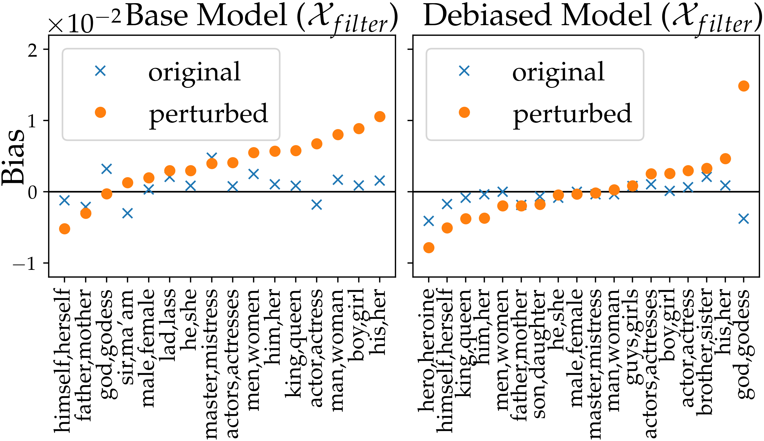 |
Our method is able to reveal the hidden model bias on , which is not visible with naive measurements. In Fig.˜5, the naive approach () observes very small biases on most tokens (as constructed). In contrast, when evaluated by our double perturbation framework (), we are able to observe noticeable bias, where most has a positive bias on the base model. This observed bias is in line with the measurements on the original (Section˜A.4), indicating that we reveal the correct model bias. Furthermore, we observe mitigated biases in the debiased model, which demonstrates the effectiveness of data augmentation.
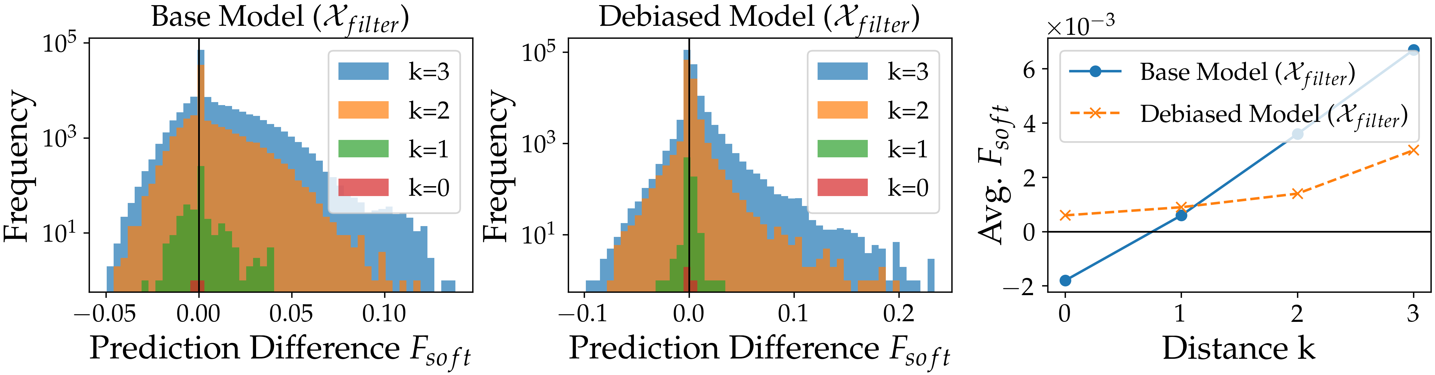
To demonstrate how our method reveals hidden bias, we conduct a case study with and show the relationship between the bias and the neighborhood distance . We present the histograms for in Fig.˜6 and plot the corresponding vs. in the right-most panel. Surprisingly, for the base model, the bias is negative when , but becomes positive when . This is because the naive approach only has two test examples (Table˜5) thus the measurement is not robust. In contrast, our method is able to construct similar natural sentences when and shifts the distribution to the right (positive). As shown in the right-most panel, the bias is small when , and becomes more significant as increases (larger neighborhood). As discussed in Section˜4.1, the neighborhood construction does not introduce additional bias, and these results demonstrate the effectiveness of our method in revealing hidden model bias.
5 Related Work
First-order robustness evaluation. A line of work has been proposed to study the vulnerability of natural language models, through transformations such as character-level perturbations (Ebrahimi et al., 2018), word-level perturbations (Jin et al., 2019; Ren et al., 2019; Yang et al., 2020; Hsieh et al., 2019; Cheng et al., 2020; Li et al., 2020), prepending or appending a sequence (Jia and Liang, 2017; Wallace et al., 2019a), and generative models (Zhao et al., 2018b). They focus on constructing adversarial examples from the test set that alter the prediction, whereas our methods focus on finding vulnerable examples beyond the test set whose predictions can be altered.
Robustness beyond the test set. Several works have studied model robustness beyond test sets but mostly focused on computer vision tasks. Zhang et al. (2019) demonstrate that a robustly trained model could still be vulnerable to small perturbations if the input comes from a distribution only slightly different than a normal test set (e.g., images with slightly different contrasts). Hendrycks and Dietterich (2019) study more sources of common corruptions such as brightness, motion blur and fog. Unlike in computer vision where simple image transformations can be used, in our natural language setting, generating a valid example beyond test set is more challenging because language semantics and grammar must be maintained.
Counterfactual fairness. Kusner et al. (2017) propose counterfactual fairness and consider a model fair if changing the protected attributes does not affect the distribution of prediction. We follow the definition and focus on evaluating the counterfactual bias between pairs of protected tokens. Existing literature quantifies fairness on a test dataset or through templates (Feldman et al., 2015; Kiritchenko and Mohammad, 2018; May et al., 2019; Huang et al., 2020). For instance, Garg et al. (2019) quantify the absolute counterfactual token fairness gap on the test set; Prabhakaran et al. (2019) study perturbation sensitivity for named entities on a given set of corpus. Wallace et al. (2019b); Sheng et al. (2019, 2020) study how language generation models respond differently to prompt sentences containing mentions of different demographic groups. In contrast, our method quantifies the bias on the constructed neighborhood.
6 Conclusion
This work proposes the double perturbation framework to identify model weaknesses beyond the test dataset, and study a stronger notion of robustness and counterfactual bias. We hope that our work can stimulate the research on further improving the robustness and fairness of natural language models.
Acknowledgments
We thank anonymous reviewers for their helpful feedback. We thank UCLA-NLP group for the valuable discussions and comments. The research is supported NSF #1927554, #1901527, #2008173 and #2048280 and an Amazon Research Award.
Ethical Considerations
Intended use. One primary goal of NLP models is the generalization to real-world inputs. However, existing test datasets and templates are often not comprehensive, and thus it is difficult to evaluate real-world performance (Recht et al., 2019; Ribeiro et al., 2020). Our work sheds a light on quantifying performance for inputs beyond the test dataset and help uncover model weaknesses prior to the real-world deployment.
Misuse potential. Similar to other existing adversarial attack methods (Ebrahimi et al., 2018; Jin et al., 2019; Zhao et al., 2018b), our second-order attacks can be used for finding vulnerable examples to a NLP system. Therefore, it is essential to study how to improve the robustness of NLP models against second-order attacks.
Limitations. While the core idea about the double perturbation framework is general, in Section˜4, we consider only binary gender in the analysis of counterfactual fairness due to the restriction of the English corpus we used, which only have words associated with binary gender such as he/she, waiter/waitress, etc.
References
- Alzantot et al. (2018) Moustafa Alzantot, Yash Sharma, Ahmed Elgohary, Bo-Jhang Ho, Mani Srivastava, and Kai-Wei Chang. 2018. Generating natural language adversarial examples. In Proceedings of the 2018 Conference on Empirical Methods in Natural Language Processing, pages 2890–2896, Brussels, Belgium. Association for Computational Linguistics.
- Cheng et al. (2020) Minhao Cheng, Jinfeng Yi, Pin-Yu Chen, Huan Zhang, and Cho-Jui Hsieh. 2020. Seq2sick: Evaluating the robustness of sequence-to-sequence models with adversarial examples. Proceedings of the AAAI Conference on Artificial Intelligence, 34(04):3601–3608.
- Dixon et al. (2018) Lucas Dixon, John Li, Jeffrey Sorensen, Nithum Thain, and Lucy Vasserman. 2018. Measuring and mitigating unintended bias in text classification. In Proceedings of the 2018 AAAI/ACM Conference on AI, Ethics, and Society, AIES ’18, page 67–73, New York, NY, USA. Association for Computing Machinery.
- Dvijotham et al. (2018) Krishnamurthy Dvijotham, Sven Gowal, Robert Stanforth, Relja Arandjelovic, Brendan O’Donoghue, Jonathan Uesato, and Pushmeet Kohli. 2018. Training verified learners with learned verifiers.
- Ebrahimi et al. (2018) Javid Ebrahimi, Anyi Rao, Daniel Lowd, and Dejing Dou. 2018. HotFlip: White-box adversarial examples for text classification. In Proceedings of the 56th Annual Meeting of the Association for Computational Linguistics (Volume 2: Short Papers), pages 31–36, Melbourne, Australia. Association for Computational Linguistics.
- Feldman et al. (2015) Michael Feldman, Sorelle A Friedler, John Moeller, Carlos Scheidegger, and Suresh Venkatasubramanian. 2015. Certifying and removing disparate impact. In proceedings of the 21th ACM SIGKDD international conference on knowledge discovery and data mining, pages 259–268.
- Garg et al. (2019) Sahaj Garg, Vincent Perot, Nicole Limtiaco, Ankur Taly, Ed H. Chi, and Alex Beutel. 2019. Counterfactual fairness in text classification through robustness. In Proceedings of the 2019 AAAI/ACM Conference on AI, Ethics, and Society, AIES ’19, page 219–226, New York, NY, USA. Association for Computing Machinery.
- Garg and Ramakrishnan (2020) Siddhant Garg and Goutham Ramakrishnan. 2020. BAE: BERT-based adversarial examples for text classification. In Proceedings of the 2020 Conference on Empirical Methods in Natural Language Processing (EMNLP), pages 6174–6181, Online. Association for Computational Linguistics.
- Hendrycks and Dietterich (2019) Dan Hendrycks and Thomas Dietterich. 2019. Benchmarking neural network robustness to common corruptions and perturbations. In International Conference on Learning Representations.
- Hsieh et al. (2019) Yu-Lun Hsieh, Minhao Cheng, Da-Cheng Juan, Wei Wei, Wen-Lian Hsu, and Cho-Jui Hsieh. 2019. On the robustness of self-attentive models. In Proceedings of the 57th Annual Meeting of the Association for Computational Linguistics, pages 1520–1529.
- Huang and Chang (2021) Kuan-Hao Huang and Kai-Wei Chang. 2021. Generating syntactically controlled paraphrases without using annotated parallel pairs. In EACL.
- Huang et al. (2019) Po-Sen Huang, Robert Stanforth, Johannes Welbl, Chris Dyer, Dani Yogatama, Sven Gowal, Krishnamurthy Dvijotham, and Pushmeet Kohli. 2019. Achieving verified robustness to symbol substitutions via interval bound propagation. Proceedings of the 2019 Conference on Empirical Methods in Natural Language Processing and the 9th International Joint Conference on Natural Language Processing (EMNLP-IJCNLP).
- Huang et al. (2020) Po-Sen Huang, Huan Zhang, Ray Jiang, Robert Stanforth, Johannes Welbl, Jack Rae, Vishal Maini, Dani Yogatama, and Pushmeet Kohli. 2020. Reducing sentiment bias in language models via counterfactual evaluation. Findings in EMNLP.
- Iyyer et al. (2018) Mohit Iyyer, J. Wieting, Kevin Gimpel, and Luke Zettlemoyer. 2018. Adversarial example generation with syntactically controlled paraphrase networks. ArXiv, abs/1804.06059.
- Jia and Liang (2017) Robin Jia and Percy Liang. 2017. Adversarial examples for evaluating reading comprehension systems. In Proceedings of the 2017 Conference on Empirical Methods in Natural Language Processing, EMNLP 2017, Copenhagen, Denmark, September 9-11, 2017, pages 2021–2031. Association for Computational Linguistics.
- Jia et al. (2019) Robin Jia, Aditi Raghunathan, Kerem Göksel, and Percy Liang. 2019. Certified robustness to adversarial word substitutions. In EMNLP/IJCNLP.
- Jin et al. (2019) Di Jin, Zhijing Jin, Joey Tianyi Zhou, and Peter Szolovits. 2019. Is bert really robust? a strong baseline for natural language attack on text classification and entailment.
- Kiritchenko and Mohammad (2018) Svetlana Kiritchenko and Saif Mohammad. 2018. Examining gender and race bias in two hundred sentiment analysis systems. In Proceedings of the Seventh Joint Conference on Lexical and Computational Semantics, pages 43–53, New Orleans, Louisiana. Association for Computational Linguistics.
- Kusner et al. (2017) Matt J Kusner, Joshua Loftus, Chris Russell, and Ricardo Silva. 2017. Counterfactual fairness. In I. Guyon, U. V. Luxburg, S. Bengio, H. Wallach, R. Fergus, S. Vishwanathan, and R. Garnett, editors, Advances in Neural Information Processing Systems 30, pages 4066–4076. Curran Associates, Inc.
- Li et al. (2020) Linyang Li, Ruotian Ma, Qipeng Guo, Xiangyang Xue, and Xipeng Qiu. 2020. BERT-ATTACK: Adversarial attack against BERT using BERT. In Proceedings of the 2020 Conference on Empirical Methods in Natural Language Processing (EMNLP), pages 6193–6202, Online. Association for Computational Linguistics.
- May et al. (2019) Chandler May, Alex Wang, Shikha Bordia, Samuel R. Bowman, and Rachel Rudinger. 2019. On measuring social biases in sentence encoders. In Proceedings of the 2019 Conference of the North American Chapter of the Association for Computational Linguistics: Human Language Technologies, Volume 1 (Long and Short Papers), pages 622–628, Minneapolis, Minnesota. Association for Computational Linguistics.
- Miyato et al. (2017) Takeru Miyato, Andrew M. Dai, and Ian Goodfellow. 2017. Adversarial training methods for semi-supervised text classification. ICLR.
- Morris et al. (2020) John X. Morris, Eli Lifland, Jin Yong Yoo, Jake Grigsby, Di Jin, and Yanjun Qi. 2020. Textattack: A framework for adversarial attacks, data augmentation, and adversarial training in nlp.
- Mrkšić et al. (2016) Nikola Mrkšić, Diarmuid Ó Séaghdha, Blaise Thomson, Milica Gašić, Lina M. Rojas-Barahona, Pei-Hao Su, David Vandyke, Tsung-Hsien Wen, and Steve Young. 2016. Counter-fitting word vectors to linguistic constraints. In Proceedings of the 2016 Conference of the North American Chapter of the Association for Computational Linguistics: Human Language Technologies, pages 142–148, San Diego, California. Association for Computational Linguistics.
- Pennington et al. (2014) Jeffrey Pennington, Richard Socher, and Christopher D. Manning. 2014. Glove: Global vectors for word representation. In Empirical Methods in Natural Language Processing (EMNLP), pages 1532–1543.
- Prabhakaran et al. (2019) Vinodkumar Prabhakaran, Ben Hutchinson, and Margaret Mitchell. 2019. Perturbation sensitivity analysis to detect unintended model biases. In Proceedings of the 2019 Conference on Empirical Methods in Natural Language Processing and the 9th International Joint Conference on Natural Language Processing (EMNLP-IJCNLP), pages 5740–5745, Hong Kong, China. Association for Computational Linguistics.
- Radford et al. (2019) Alec Radford, Jeff Wu, Rewon Child, David Luan, Dario Amodei, and Ilya Sutskever. 2019. Language models are unsupervised multitask learners.
- Recht et al. (2019) Benjamin Recht, Rebecca Roelofs, Ludwig Schmidt, and Vaishaal Shankar. 2019. Do ImageNet classifiers generalize to ImageNet? volume 97 of Proceedings of Machine Learning Research, pages 5389–5400, Long Beach, California, USA. PMLR.
- Ren et al. (2019) Shuhuai Ren, Yihe Deng, Kun He, and Wanxiang Che. 2019. Generating natural language adversarial examples through probability weighted word saliency. In Proceedings of the 57th Annual Meeting of the Association for Computational Linguistics, pages 1085–1097, Florence, Italy. Association for Computational Linguistics.
- Ribeiro et al. (2020) Marco Tulio Ribeiro, Tongshuang Wu, Carlos Guestrin, and Sameer Singh. 2020. Beyond accuracy: Behavioral testing of nlp models with checklist. In Association for Computational Linguistics (ACL).
- Sanh et al. (2019) Victor Sanh, Lysandre Debut, Julien Chaumond, and Thomas Wolf. 2019. Distilbert, a distilled version of bert: smaller, faster, cheaper and lighter. ArXiv, abs/1910.01108.
- Sheng et al. (2019) Emily Sheng, Kai-Wei Chang, Premkumar Natarajan, and Nanyun Peng. 2019. The woman worked as a babysitter: On biases in language generation. In EMNLP.
- Sheng et al. (2020) Emily Sheng, Kai-Wei Chang, Premkumar Natarajan, and Nanyun Peng. 2020. Towards controllable biases in language generation. In EMNLP-Finding.
- Shi et al. (2020) Zhouxing Shi, Huan Zhang, Kai-Wei Chang, Minlie Huang, and Cho-Jui Hsieh. 2020. Robustness verification for transformers. In International Conference on Learning Representations.
- Socher et al. (2013) Richard Socher, Alex Perelygin, Jean Wu, Jason Chuang, Christopher D. Manning, Andrew Ng, and Christopher Potts. 2013. Recursive deep models for semantic compositionality over a sentiment treebank. In Proceedings of the 2013 Conference on Empirical Methods in Natural Language Processing, pages 1631–1642, Seattle, Washington, USA. Association for Computational Linguistics.
- Wallace et al. (2019a) Eric Wallace, Shi Feng, Nikhil Kandpal, Matt Gardner, and Sameer Singh. 2019a. Universal adversarial triggers for attacking and analyzing nlp. In EMNLP/IJCNLP.
- Wallace et al. (2019b) Eric Wallace, Shi Feng, Nikhil Kandpal, Matt Gardner, and Sameer Singh. 2019b. Universal adversarial triggers for attacking and analyzing NLP. In EMNLP.
- Wang et al. (2019) Alex Wang, Amanpreet Singh, Julian Michael, Felix Hill, Omer Levy, and Samuel R. Bowman. 2019. Glue: A multi-task benchmark and analysis platform for natural language understanding.
- Wolf et al. (2020) Thomas Wolf, Lysandre Debut, Victor Sanh, Julien Chaumond, Clement Delangue, Anthony Moi, Pierric Cistac, Tim Rault, Rémi Louf, Morgan Funtowicz, Joe Davison, Sam Shleifer, Patrick von Platen, Clara Ma, Yacine Jernite, Julien Plu, Canwen Xu, Teven Le Scao, Sylvain Gugger, Mariama Drame, Quentin Lhoest, and Alexander M. Rush. 2020. Huggingface’s transformers: State-of-the-art natural language processing.
- Xu et al. (2020) Kaidi Xu, Zhouxing Shi, Huan Zhang, Yihan Wang, Kai-Wei Chang, Minlie Huang, Bhavya Kailkhura, Xue Lin, and Cho-Jui Hsieh. 2020. Automatic perturbation analysis for scalable certified robustness and beyond.
- Yang et al. (2020) Puyudi Yang, Jianbo Chen, Cho-Jui Hsieh, Jane-Ling Wang, and Michael I. Jordan. 2020. Greedy attack and gumbel attack: Generating adversarial examples for discrete data. Journal of Machine Learning Research, 21(43):1–36.
- Zang et al. (2020) Yuan Zang, Fanchao Qi, Chenghao Yang, Zhiyuan Liu, Meng Zhang, Qun Liu, and Maosong Sun. 2020. Word-level textual adversarial attacking as combinatorial optimization. Proceedings of the 58th Annual Meeting of the Association for Computational Linguistics.
- Zhang et al. (2019) Huan Zhang, Hongge Chen, Zhao Song, Duane Boning, inderjit dhillon, and Cho-Jui Hsieh. 2019. The limitations of adversarial training and the blind-spot attack. In International Conference on Learning Representations.
- Zhao et al. (2019) Jieyu Zhao, Tianlu Wang, Mark Yatskar, Ryan Cotterell, Vicente Ordonez, and Kai-Wei Chang. 2019. Gender bias in contextualized word embeddings. In NAACL.
- Zhao et al. (2018a) Jieyu Zhao, Tianlu Wang, Mark Yatskar, Vicente Ordonez, and Kai-Wei Chang. 2018a. Gender bias in coreference resolution: Evaluation and debiasing methods. In Proceedings of the 2018 Conference of the North American Chapter of the Association for Computational Linguistics: Human Language Technologies, Volume 2 (Short Papers), pages 15–20, New Orleans, Louisiana. Association for Computational Linguistics.
- Zhao et al. (2018b) Zhengli Zhao, Dheeru Dua, and Sameer Singh. 2018b. Generating natural adversarial examples. In International Conference on Learning Representations.
- Zhou et al. (2020) Yi Zhou, Xiaoqing Zheng, Cho-Jui Hsieh, Kai-Wei Chang, and Xuanjing Huang. 2020. Defense against adversarial attacks in nlp via dirichlet neighborhood ensemble. arXiv preprint arXiv:2006.11627.
Appendix A Supplemental Material
A.1 Random Baseline
To validate the effectiveness of minimizing Eq.˜4, we also experiment on a second-order baseline that constructs vulnerable examples by randomly replacing up to 6 words. We use the same masked language model and threshold as SO-Beam such that they share a similar neighborhood. We perform the attack on the same models as Table˜2, and the attack success rates on robustly trained BoW, CNN, LSTM, and Transformers are 18.8%, 22.3%, 15.2%, and 25.1%, respectively. Despite being a second-order attack, the random baseline has low attack success rates thus demonstrates the effectiveness of SO-Beam.
A.2 Human Evaluation
We randomly select 100 successful attacks from SO-Beam and consider four types of examples (for a total of 400 examples): The original examples with and without synonym substitution , and the vulnerable examples with and without synonym substitution . For each example, we annotate the naturalness and sentiment separately as described below.
Naturalness of vulnerable examples. We ask the annotators to score the likelihood of being an original example (i.e., not altered by computer) based on grammar correctness and naturalness, with a Likert scale of 1-5: (1) Sure adversarial example. (2) Likely an adversarial example. (3) Neutral. (4) Likely an original example. (5) Sure original example.
Semantic similarity after the synonym substitution. We first ask the annotators to predict the sentiment on a Likert scale of 1-5, and then map the prediction to three categories: negative, neutral, and positive. We consider two examples to have the same semantic meaning if and only if they are both positive or negative.
A.3 Running Time
We experiment with the validation split on a single RTX 3090, and measure the average running time per example. As shown in Table˜6, SO-Beam runs faster than SO-Enum since it utilizes the probability output. The running time may increase if the model has improved second-order robustness.
| Running Time (seconds) | ||||
| Genetic | BAE | SO-Enum | SO-Beam | |
| Base Models: | ||||
| BoW | 31.6 | 0.9 | 6.2 | 1.8 |
| CNN | 28.8 | 1.0 | 5.9 | 1.7 |
| LSTM | 31.9 | 1.1 | 7.0 | 1.9 |
| Transformer | 51.9 | 0.5 | 6.5 | 2.5 |
| BERT-base | 65.6 | 1.1 | 35.4 | 7.1 |
| Robust Models: | ||||
| BoW | 103.9 | 1.0 | 8.0 | 3.5 |
| CNN | 129.4 | 1.0 | 6.7 | 2.6 |
| LSTM | 116.4 | 1.1 | 10.7 | 5.3 |
| Transformer | 66.4 | 0.5 | 5.9 | 2.6 |
A.4 Additional Results on Protected Tokens
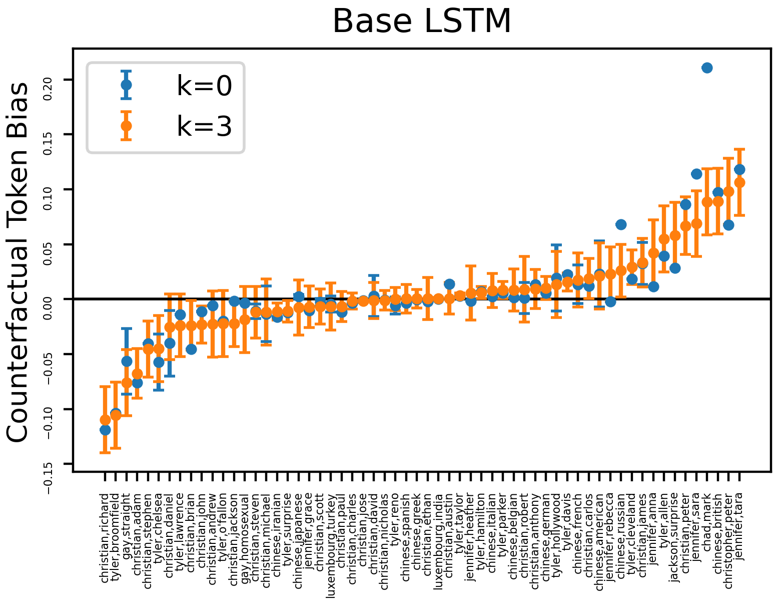
Fig.˜7 presents the experimental results with additional protected tokens such as nationality, religion, and sexual orientation (from Ribeiro et al. (2020)). We use the same base LSTM as described in Section˜4.2. One interesting observation is when where the bias is negative, indicating that the sentiment classifier tends to give more negative prediction when substituting in the input. This phenomenon is opposite to the behavior of toxicity classifiers (Dixon et al., 2018), and we hypothesize that it may be caused by the different distribution of training data. To verify the hypothesis, we count the number of training examples containing each word, and observe that we have far more negative examples than positive examples among those containing straight (Table˜7). After looking into the training set, it turns out that straight to video is a common phrase to criticize a film, thus the classifier incorrectly correlates straight with negative sentiment. This also reveals the limitation of our method on polysemous words.
| # Negative | # Positive | |
| gay | 37 | 20 |
| straight | 71 | 18 |
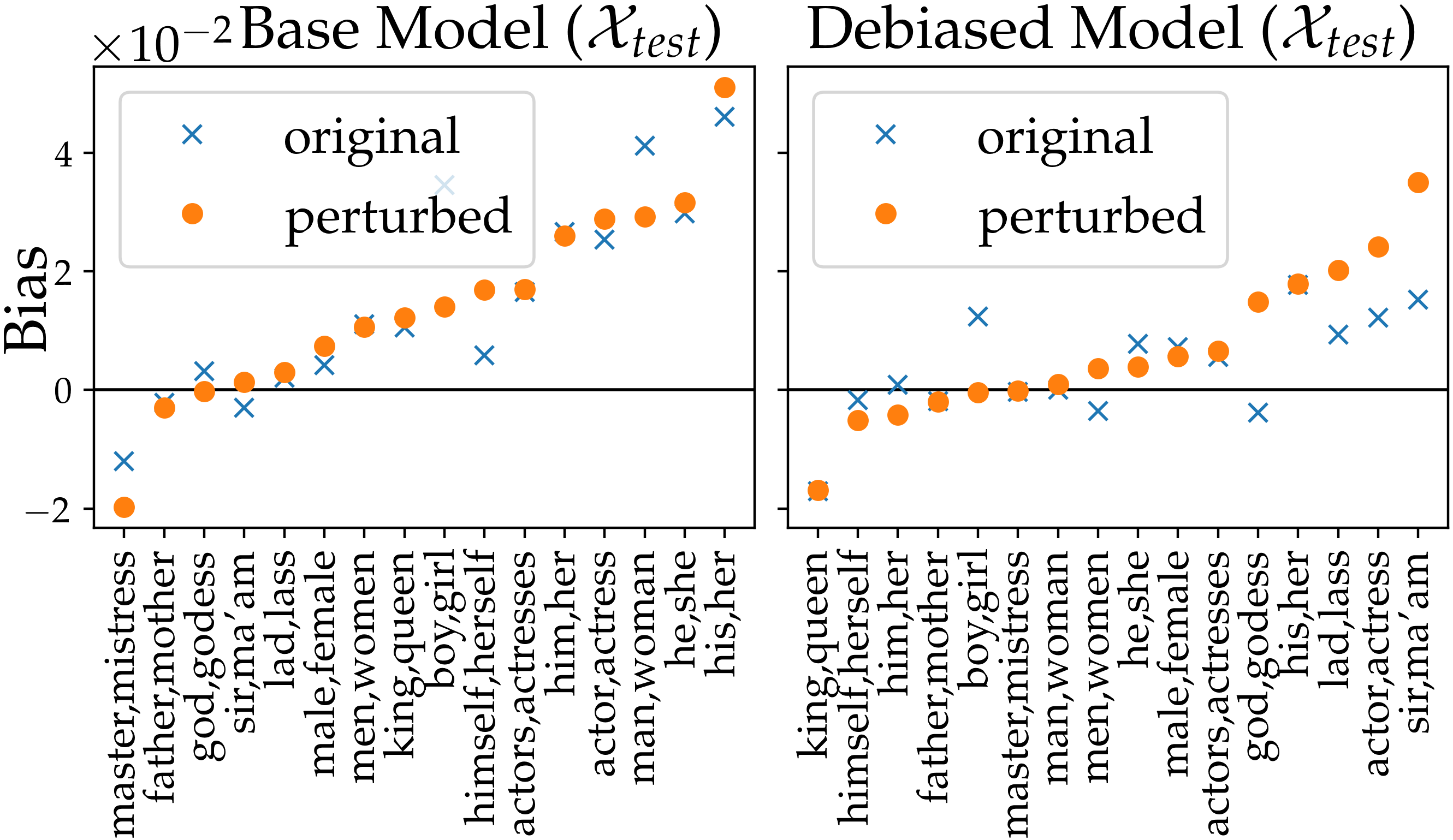
In Fig.˜8, we measure the bias on and observe positive bias on most tokens for both and , which indicates that the model “tends” to make more positive predictions for examples containing certain female pronouns than male pronouns. Notice that even though gender swap mitigates the bias to some extent, it is still difficult to fully eliminate the bias. This is probably caused by tuples like (him, his, her) which cannot be swapped perfectly, and requires additional processing such as part-of-speech resolving (Zhao et al., 2018a).
A.5 Additional Results on Robustness
Table˜8 provides the quality metrics for first-order attacks, where we measure the GPT-2 perplexity and norm distance between the input and the adversarial example. For BAE we evaluate on 872 validation examples, and for Genetic we evaluate on 100 validation examples due to the long running time.
| Genetic | BAE | |||||
| Original PPL | Perturb PPL | Original PPL | Perturb PPL | |||
| Base Models: | ||||||
| BoW | 145 | 258 | 3.3 | 192 | 268 | 1.6 |
| CNN | 146 | 282 | 3.0 | 186 | 254 | 1.5 |
| LSTM | 131 | 238 | 2.9 | 190 | 263 | 1.6 |
| Transformer | 137 | 232 | 2.8 | 185 | 254 | 1.4 |
| BERT-base | 201 | 342 | 3.4 | 189 | 277 | 1.6 |
| Robust Models: | ||||||
| BoW | 132 | 177 | 2.4 | 214 | 269 | 1.5 |
| CNN | 136 | 236 | 2.7 | 211 | 279 | 1.5 |
| LSTM | 163 | 267 | 2.5 | 220 | 302 | 1.6 |
| Transformer | 118 | 200 | 2.8 | 196 | 261 | 1.4 |
Table˜11 shows additional attack results from SO-Beam on base LSTM, and Table˜12 shows additional attack results from SO-Beam on robust CNN. Bold words are the corresponding patch words , taken from the predefined list of counter-fitted synonyms.
| Type | Predictions | Text |
| Original | 95% Negative 94% Negative | it ’s hampered by a lifetime-channel kind of plot and a lead actor (actress) who is out of their depth . |
| Distance | 97% Negative (97% Negative) | it ’s hampered by a lifetime-channel kind of plot and lone lead actor (actress) who is out of their depth . |
| 56% Negative (55% Positive ) | it ’s hampered by a lifetime-channel kind of plot and a lead actor (actress) who is out of creative depth . | |
| 89% Negative (84% Negative) | it ’s hampered by a lifetime-channel kind of plot and a lead actor (actress) who talks out of their depth . | |
| 98% Negative (98% Negative) | it ’s hampered by a lifetime-channel kind of plot and a lead actor (actress) who is out of production depth . | |
| 96% Negative (96% Negative) | it ’s hampered by a lifetime-channel kind of plot and a lead actor (actress) that is out of their depth . | |
| Distance | 88% Negative (87% Negative) | it ’s hampered by a lifetime-channel cast of stars and a lead actor (actress) who is out of their depth . |
| 96% Negative (95% Negative) | it ’s hampered by a simple set of plot and a lead actor (actress) who is out of their depth . | |
| 54% Negative (54% Negative) | it ’s framed about a lifetime-channel kind of plot and a lead actor (actress) who is out of their depth . | |
| 90% Negative (88% Negative) | it ’s hampered by a lifetime-channel mix between plot and a lead actor (actress) who is out of their depth . | |
| 78% Negative (68% Negative) | it ’s hampered by a lifetime-channel kind of plot and a lead actor (actress) who storms out of their mind . | |
| Distance | 52% Positive (64% Positive ) | it ’s characterized by a lifetime-channel combination comedy plot and a lead actor (actress) who is out of their depth . |
| 93% Negative (93% Negative) | it ’s hampered by a lifetime-channel kind of star and a lead actor (actress) who falls out of their depth . | |
| 58% Negative (57% Negative) | it ’s hampered by a tough kind of singer and a lead actor (actress) who is out of their teens . | |
| 70% Negative (52% Negative) | it ’s hampered with a lifetime-channel kind of plot and a lead actor (actress) who operates regardless of their depth . | |
| 58% Negative (53% Positive ) | it ’s hampered with a lifetime-channel cast of plot and a lead actor (actress) who is out of creative depth . |
| Type | Predictions | Text |
| Original | 55% Positive (67% Positive ) | a hamfisted romantic comedy that makes our boy (girl) the hapless facilitator of an extended cheap shot across the mason-dixon line . |
| Distance | 52% Positive (66% Positive ) | a hamfisted romantic comedy that makes our boy (girl) the hapless facilitator of an extended cheap shot from the mason-dixon line . |
| 73% Positive (79% Positive ) | a hamfisted romantic comedy that makes our boy (girl) the hapless facilitator gives an extended cheap shot across the mason-dixon line . | |
| 56% Negative (58% Positive ) | a hamfisted romantic comedy that makes our boy (girl) the hapless facilitator of an extended cheap shot across the phone line . | |
| 75% Positive (83% Positive ) | a hamfisted romantic comedy that makes our boy (girl) the hapless facilitator of an extended chase shot across the mason-dixon line . | |
| 75% Positive (81% Positive ) | a hamfisted romantic comedy that makes our boy (girl) our hapless facilitator of an extended cheap shot across the mason-dixon line . | |
| Distance | 85% Positive (85% Positive ) | a hilarious romantic comedy that makes our boy (girl) the hapless facilitator of an emotionally cheap shot across the mason-dixon line . |
| 81% Positive (86% Positive ) | a hamfisted romantic comedy romance makes our boy (girl) the hapless facilitator of an extended cheap delivery across the mason-dixon line . | |
| 84% Positive (87% Positive ) | a hamfisted romantic romance adventure makes our boy (girl) the hapless facilitator of an extended cheap shot across the mason-dixon line . | |
| 50% Negative (62% Positive ) | a hamfisted romantic comedy that makes our boy (girl) the hapless boss of an extended cheap shot behind the mason-dixon line . | |
| 77% Negative (71% Negative) | a hamfisted lesbian comedy that makes our boy (girl) the hapless facilitator of an extended slap shot across the mason-dixon line . | |
| Distance | 97% Positive (97% Positive ) | a darkly romantic comedy romance makes our boy (girl) the hapless facilitator delivers an extended cheap shot across the mason-dixon line . |
| 69% Positive (74% Positive ) | a hamfisted romantic comedy film makes our boy (girl) the hapless facilitator of an extended cheap shot across the production line . | |
| 87% Positive (89% Positive ) | a hamfisted romantic comedy that makes our boy (girl) the exclusive focus of an extended cheap shot across the mason-dixon line . | |
| 64% Positive (76% Positive ) | a hamfisted romantic comedy that makes our boy (girl) the hapless facilitator shoots an extended flash shot across the camera line . | |
| 99% Positive (99% Positive ) | a compelling romantic comedy that makes our boy (girl) the perfect facilitator of an extended story shot across the mason-dixon line . |
| Type | Predictions | Text |
| Original | 99% Positive (99% Positive ) | it ’s a charming and sometimes (often) affecting journey . |
| Vulnerable | 59% Negative (56% Positive ) | it ’s a charming and sometimes (often) painful journey . |
| Original | 99% Negative (97% Negative) | unflinchingly bleak (somber) and desperate |
| Vulnerable | 80% Negative (79% Positive ) | unflinchingly bleak (somber) and mysterious |
| Original | 99% Positive (93% Positive ) | allows us to hope that nolan is poised to embark a major career (quarry) as a commercial yet inventive filmmaker . |
| Vulnerable | 76% Positive (75% Negative) | allows us to hope that nolan is poised to embark a major career (quarry) as a commercial yet amateur filmmaker . |
| Original | 94% Positive (68% Positive ) | the acting , costumes , music , cinematography and sound are all astounding (staggering) given the production ’s austere locales . |
| Vulnerable | 87% Positive (66% Negative) | the acting , costumes , music , cinematography and sound are largely astounding (staggering) given the production ’s austere locales . |
| Original | 99% Positive (97% Positive ) | although laced with humor and a few fanciful touches , the film is a refreshingly serious look at young (juvenile) women . |
| Vulnerable | 94% Positive (81% Negative) | although laced with humor and a few fanciful touches , the film is a moderately serious look at young (juvenile) women . |
| Original | 99% Negative (98% Negative) | a sometimes (occasionally) tedious film . |
| Vulnerable | 62% Negative (55% Positive ) | a sometimes (occasionally) disturbing film . |
| Original | 100% Negative (100% Negative) | in exactly 89 minutes , most of which passed as slowly as if i ’d been sitting naked on an igloo , formula 51 sank from quirky (lunatic) to jerky to utter turkey . |
| Vulnerable | 51% Positive (65% Negative) | lasting exactly 89 minutes , most of which passed as slowly as if i ’d been sitting naked on an igloo , but 51 ranges from quirky (lunatic) to delicious to crisp turkey . |
| Original | 97% Positive (100% Positive ) | the scintillating (mesmerizing) performances of the leads keep the film grounded and keep the audience riveted . |
| Vulnerable | 91% Negative (90% Positive ) | the scintillating (mesmerizing) performances of the leads keep the film grounded and keep the plot predictable . |
| Original | 89% Negative (96% Negative) | it takes a uncanny (strange) kind of laziness to waste the talents of robert forster , anne meara , eugene levy , and reginald veljohnson all in the same movie . |
| Vulnerable | 80% Positive (76% Negative) | it takes a uncanny (strange) kind of humour to waste the talents of robert forster , anne meara , eugene levy , and reginald veljohnson all in the same movie . |
| Original | 100% Negative (100% Negative) | … the film suffers from a lack of humor ( something needed to balance (equilibrium) out the violence ) … |
| Vulnerable | 76% Positive (86% Negative) | … the film derives from a lot of humor ( something clever to balance (equilibrium) out the violence ) … |
| Original | 55% Positive (97% Positive ) | we root for ( clara and paul ) , even like them , though perhaps it ’s an emotion closer to pity (compassion) . |
| Vulnerable | 89% Negative (91% Positive ) | we root for ( clara and paul ) , even like them , though perhaps it ’s an explanation closer to pity (compassion) . |
| Original | 95% Negative (97% Negative) | even horror fans (stalkers) will most likely not find what they ’re seeking with trouble every day ; the movie lacks both thrills and humor . |
| Vulnerable | 61% Positive (59% Negative) | even horror fans (stalkers) will most likely not find what they ’re seeking with trouble every day ; the movie has both thrills and humor . |
| Original | 100% Positive (100% Positive ) | a gorgeous , high-spirited musical from india that exquisitely mixed (blends) music , dance , song , and high drama . |
| Vulnerable | 87% Negative (81% Positive ) | a dark , high-spirited musical from nowhere that loosely mixed (blends) music , dance , song , and high drama . |
| Original | 99% Negative (94% Negative) | … the movie is just a plain old (longtime) monster . |
| Vulnerable | 94% Negative (94% Positive ) | … the movie is just a pretty old (longtime) monster . |
| Type | Predictions | Text |
| Original | 54% Positive (69% Positive ) | for the most part , director anne-sophie birot ’s first feature is a sensitive , overly (extraordinarily) well-acted drama . |
| Vulnerable | 53% Negative (62% Positive ) | for the most part , director anne-sophie benoit ’s first feature is a sensitive , overly (extraordinarily) well-acted drama . |
| Original | 66% Positive (72% Positive ) | mr. tsai is a very original painter (artist) in his medium , and what time is it there ? |
| Vulnerable | 52% Negative (55% Positive ) | mr. tsai is a very original painter (artist) in his medium , and what time was it there ? |
| Original | 80% Positive (64% Positive ) | sade is an engaging (engage) look at the controversial eponymous and fiercely atheistic hero . |
| Vulnerable | 53% Positive (66% Negative) | sade is an engaging (engage) look at the controversial eponymous or fiercely atheistic hero . |
| Original | 50% Negative (57% Negative) | so devoid of any kind of comprehensible (intelligible) story that it makes films like xxx and collateral damage seem like thoughtful treatises |
| Vulnerable | 53% Positive (54% Negative) | so devoid of any kind of comprehensible (intelligible) story that it makes films like xxx and collateral 2 seem like thoughtful treatises |
| Original | 90% Positive (87% Positive ) | a tender , heartfelt (deepest) family drama . |
| Vulnerable | 60% Positive (61% Negative) | a somber , heartfelt (deepest) funeral drama . |
| Original | 57% Positive (69% Positive ) | … a hollow joke (giggle) told by a cinematic gymnast having too much fun embellishing the misanthropic tale to actually engage it . |
| Vulnerable | 56% Negative (56% Positive ) | … a hollow joke (giggle) told by a cinematic gymnast having too much fun embellishing the misanthropic tale cannot actually engage it . |
| Original | 73% Negative (56% Negative) | the cold (colder) turkey would ’ve been a far better title . |
| Vulnerable | 61% Negative (62% Positive ) | the cold (colder) turkey might ’ve been a far better title . |
| Original | 70% Negative (65% Negative) | it ’s just disappointingly superficial – a movie that has all the elements necessary to be a fascinating , involving character study , but never does more than scratch the shallow (surface) . |
| Vulnerable | 52% Negative (55% Positive ) | it ’s just disappointingly short – a movie that has all the elements necessary to be a fascinating , involving character study , but never does more than scratch the shallow (surface) . |
| Original | 79% Negative (72% Negative) | schaeffer has to find some hook on which to hang his persistently useless movies , and it might as well be the resuscitation (revival) of the middle-aged character . |
| Vulnerable | 57% Negative (57% Positive ) | schaeffer has to find some hook on which to hang his persistently entertaining movies , and it might as well be the resuscitation (revival) of the middle-aged character . |
| Original | 64% Positive (58% Positive ) | the primitive force of this film seems to bubble up from the vast collective memory of the combatants (militants) . |
| Vulnerable | 52% Positive (53% Negative) | the primitive force of this film seems to bubble down from the vast collective memory of the combatants (militants) . |
| Original | 64% Positive (74% Positive ) | on this troublesome (tricky) topic , tadpole is very much a step in the right direction , with its blend of frankness , civility and compassion . |
| Vulnerable | 55% Negative (56% Positive ) | on this troublesome (tricky) topic , tadpole is very much a step in the right direction , losing its blend of frankness , civility and compassion . |
| Original | 74% Positive (60% Positive ) | if you ’re hard (laborious) up for raunchy college humor , this is your ticket right here . |
| Vulnerable | 60% Positive (57% Negative) | if you ’re hard (laborious) up for raunchy college humor , this is your ticket holder here . |
| Original | 94% Positive (97% Positive ) | a fast , funny , highly fun (enjoyable) movie . |
| Vulnerable | 54% Negative (65% Positive ) | a dirty , violent , highly fun (enjoyable) movie . |
| Original | 86% Positive (88% Positive ) | good old-fashioned slash-and-hack is back (backwards) ! |
| Vulnerable | 52% Negative (55% Positive ) | a old-fashioned slash-and-hack is back (backwards) ! |