Doubly heavy tetraquarks in a chiral-diquark picture

Following Ref. Kim et al. (2021), we consider the chiral effective theory of diquarks given by the chiral effective Lagrangian,

$\displaystyle\mathcal{L}=\mathcal{L}_{S}+\mathcal{L}_{V}+\frac{1}{4}{\rm Tr}[\partial^{\mu}\Sigma^{\dagger}\partial_{\mu}\Sigma]-V(\Sigma)+\mathcal{L}_{V-S}.$

(1)

Here the first term $\mathcal{L}_{S}$ describes the effective Lagrangian for the scalar and pseudoscalar diquarks, and $\mathcal{L}_{V}$ for the vector and axial-vector diquarks. Their explicit forms are given below. The last term, $\mathcal{L}_{V-S}$, describes the coupling between the scalar and vector diquarks. As it does not contribute to the diquark masses, here we omit this term. The third and forth terms of Eq. (1) are the kinetic and potential terms for the meson field $\Sigma$, respectively. This meson operator $\Sigma$ contains nonet scalar $\sigma$ and pseudoscalar $\pi$ mesons, whose chiral transform is given by

$$\Sigma_{ij}=\sigma_{ij}+i\pi_{ij}\rightarrow U_{L,ik}\Sigma_{km}U^{{\dagger}}_{R,mj}.$$

(2)

The potential term for the $\Sigma$ meson field, $V(\Sigma)$, causes spontaneous chiral symmetry breaking, represented by the vacuum expectation value of scalar meson $\sigma$ as

$$\langle\Sigma_{ij}\rangle=\langle\sigma_{ij}\rangle=f_{\pi}\delta_{ij}~{},~{}~{}~{}\langle\pi_{ij}\rangle=0,$$

(3)

where $f_{\pi}\simeq 92$ MeV is the pion decay constant. In this vacuum, $\pi$ meson is regarded as the massless Nambu-Goldstone bosons.

Using the $\Sigma$ meson field and the chiral diquark operators summarized in Table. 1, the effective Lagrangians, $\mathcal{L}_{S}$ and $\mathcal{L}_{V}$, are expressed as

$\displaystyle\begin{split}\mathcal{L}_{S}&=\mathcal{D}_{\mu}d_{R,i}(\mathcal{D}^{\mu}d_{R,i})^{\dagger}+\mathcal{D}_{\mu}d_{L,i}(\mathcal{D}^{\mu}d_{L,i})^{\dagger}\\ &-m_{S0}^{2}(d_{R,i}d_{R,i}^{\dagger}+d_{L,i}d_{L,i}^{\dagger})\\ &-\frac{m_{S1}^{2}}{f_{\pi}}(d_{R,i}\Sigma_{ij}^{\dagger}d_{L,j}^{\dagger}+d_{L,i}\Sigma_{ij}d_{R,j}^{\dagger})\\ &-\frac{m_{S2}^{2}}{2f_{\pi}^{2}}\epsilon_{ijk}\epsilon_{lmn}(d_{R,k}\Sigma_{li}\Sigma_{mj}d_{L,n}^{\dagger}+d_{L,k}\Sigma^{\dagger}_{li}\Sigma^{\dagger}_{m,j}d_{R,n}^{\dagger}),\\ \end{split}$

(4)

$\displaystyle\begin{split}\mathcal{L}_{V}&=\frac{1}{2}{\rm Tr}[F^{\mu\nu}F^{{\dagger}}_{\mu\nu}]+m_{V0}^{2}{\rm Tr}[d^{\mu}d^{{\dagger}}_{\mu}]\\ &+\frac{m_{V1}^{2}}{f_{\pi}^{2}}{\rm Tr}[\Sigma^{{\dagger}}d^{\mu}\Sigma^{T}d^{{\dagger}T}_{\mu}]\\ &+\frac{m_{V2}^{2}}{f_{\pi}^{2}}[{\rm Tr}\{\Sigma^{T}\Sigma^{{\dagger}T}d_{\mu}^{{\dagger}}d^{\mu}\}+{\rm Tr}\{\Sigma\Sigma^{{\dagger}}d^{\mu}d^{{\dagger}}_{\mu}\}].\\ \end{split}$

(5)

Since the diquark is not a color-singlet state, we introduce the color-gauge-covariant derivative, $\mathcal{D}^{\mu}=\partial^{\mu}+igT^{\alpha}G^{\alpha,\mu}$, with $G^{\alpha,\mu}$ being the gluon field and $T^{\alpha}$ being the color $SU(3)$ generator for the color $\bf\bar{3}$ representation. It is used for the kinetic term of these Lagrangians. $F^{\mu\nu}=\mathcal{D}^{\mu}d^{\nu}-\mathcal{D}^{\nu}d^{\mu}$ in the first term of Eq. (5) shows the strength of chiral vector diquark fields. The self-interaction terms of gluons are omitted, and all the color indices are contracted and not explicitly written.

The masses of scalar and pseudoscalar diquarks are given by the three parameters $m_{S0}^{2}$, $m_{S1}^{2}$, and $m_{S2}^{2}$ in Eq. (4). $m_{S0}$ is the chiral invariant mass which is the degenerate mass for the two diquarks in the chiral symmetry restored phase. Mass splitting between diquarks induced by the chiral symmetry breaking is given by $m_{S1}$ and $m_{S2}$. In particular, the $m_{S1}^{2}$ term also causes the $U_{A}(1)$ symmetry breaking ’t Hooft (1976, 1986). On the other hand, the masses of vector and axial-vector diquarks are given by three parameters $m_{V0}^{2}$, $m_{V1}^{2}$, and $m_{V2}^{2}$ in Eq. (5). Similar to the scalar and pseudoscalar diquarks, $m_{V0}$ is the chiral invariant mass of vector and axial-vector diquarks, and their mass splitting is given by $m_{V1}$ and $m_{V2}$.

The non-zero strange quark mass brings about the explicit chiral symmetry breaking and the flavor $SU(3)$ symmetry breaking. In this term, the masses of scalar and pseudoscalar diquarks, $M(0^{+})$ and $M(0^{-})$, are expressed in Ref. Harada et al. (2020) as

	$\displaystyle\left[M_{ud}(0^{+})\right]^{2}$		$\displaystyle=m_{S0}^{2}-(1+\epsilon)m_{S1}^{2}-m_{S2}^{2},$		(6)
	$\displaystyle\left[M_{ns}(0^{+})\right]^{2}$		$\displaystyle=m_{S0}^{2}-m_{S1}^{2}-(1+\epsilon)m_{S2}^{2},$		(7)
	$\displaystyle\left[M_{ud}(0^{-})\right]^{2}$		$\displaystyle=m_{S0}^{2}+(1+\epsilon)m_{S1}^{2}+m_{S2}^{2},$		(8)
	$\displaystyle\left[M_{ns}(0^{-})\right]^{2}$		$\displaystyle=m_{S0}^{2}+m_{S1}^{2}+(1+\epsilon)m_{S2}^{2},$		(9)

where the index $n$ stands for $u$ or $d$ quark, and $s$ for $s$ quark, meaning two constituent quarks of a diquark. The constant $\epsilon$ is given by

$\displaystyle\epsilon=\frac{f_{s}}{f_{\pi}}\left(1+\frac{m_{s}-g_{s}f_{\pi}}{g_{s}f_{s}}\right)\simeq 2/3,$

(10)

with $f_{s}=2f_{K}-f_{\pi}$, where $m_{s},g_{s},f_{\pi}$, and $f_{K}$ stands for the mass of strange quark, the quark-meson coupling constant, and the decay constants of pion and kaon, respectively. From these mass formulas, Eqs. (6)–(9), we can give the mass relation of scalar and pseudoscalar diquarks Harada et al. (2020); Kim et al. (2020, 2021) as

	$\displaystyle[M_{ns}(0^{+})]^{2}-[M_{ud}(0^{+})]^{2}=[M_{ud}(0^{-})]^{2}-$		$\displaystyle[M_{ns}(0^{-})]^{2}$		(11)
			$\displaystyle>0.$

From Eq. (11), we see the non-strange pseudoscalar diquark is heavier than the singly strange pseudoscalar diquark, $M_{ud}(0^{-})>M_{ns}(0^{-})$, which is called the inverse mass hierarchy.

The masses of axial-vector and vector diquarks, $M(1^{+})$ and $M(1^{-})$, are expressed in Ref. Kim et al. (2021) as

	$\displaystyle\left[M_{nn}(1^{+})\right]^{2}$		$\displaystyle=m_{V0}^{2}+m_{V1}^{2}+2m_{V2}^{2},$		(12)
	$\displaystyle\left[M_{ns}(1^{+})\right]^{2}$		$\displaystyle=m_{V0}^{2}+m_{V1}^{2}+2m_{V2}^{2}$		(13)
			$\displaystyle+\epsilon(m_{V1}^{2}+2m_{V2}^{2}),$
	$\displaystyle\left[M_{ss}(1^{+})\right]^{2}$		$\displaystyle=m_{V0}^{2}+m_{V1}^{2}+2m_{V2}^{2}$		(14)
			$\displaystyle+2\epsilon(m_{V1}^{2}+2m_{V2}^{2}),$
	$\displaystyle\left[M_{ud}(1^{-})\right]^{2}$		$\displaystyle=m_{V0}^{2}-m_{V1}^{2}+2m_{V2}^{2},$		(15)
	$\displaystyle\left[M_{ns}(1^{-})\right]^{2}$		$\displaystyle=m_{V0}^{2}-m_{V1}^{2}+2m_{V2}^{2}$		(16)
			$\displaystyle+\epsilon(-m_{V1}^{2}+2m_{V2}^{2}).$

For the masses of axial-vector diquarks, Eqs. (12)–(14), the generalized Gell-Mann–Okubo mass formula Kim et al. (2021) which is analogous to the conventional one Gell-Mann (1962); Okubo (1962) is obtained as

	$\displaystyle[M_{ss}(1^{+})]^{2}-[M_{ns}(1^{+})]^{2}$		$\displaystyle=[M_{ns}(1^{+})]^{2}-[M_{nn}(1^{+})]^{2}$		(17)
			$\displaystyle=\epsilon(m_{V1}^{2}+2m_{V2}^{2}).$

Here the square mass differences are characterized by the number of $s$ quark. On the other hand, the square mass difference between nonstrange and singly strange vector diquarks is given by

$\displaystyle[M_{ns}(1^{-})]^{2}-[M_{ud}(1^{-})]^{2}=\epsilon(-m_{V1}^{2}+2m_{V2}^{2}).$

(18)

As shown in Table. 2, the parameter $m_{V1}^{2}$ generally takes the negative value Kim et al. (2021), so that the mass difference between nonstrange and singly strange vector diquarks becomes much larger than that of axial-vector diquarks. Here we call this the enhanced mass hierarchy of vector diquarks in this paper.

In order to calculate the spectrum of $T_{QQ}$ tetraquarks, we use the chiral effective theory of diquark Harada et al. (2020); Kim et al. (2020, 2021) and consider these tetraquarks as the three-body system with two heavy quarks ($Q_{1},Q_{2}$) and one antidiquark ($\bar{d}$). We need two kinds of two-body potentials, one for the interaction between two heavy quarks, $V_{Q_{1}Q_{2}}$, and the other for between a heavy quark and a color $\bm{3}$ antidiquark, $V_{Q_{i}\bar{d}}$.

The Hamiltonian for this tetraquark system is written as

	$\displaystyle H=\sum_{k=\{Q_{1},Q_{2},\bar{d}\}}$		$\displaystyle\left(M_{k}+\frac{\bm{p}_{k}^{2}}{2M_{k}}\right)-K_{c.m.}$		(19)
			$\displaystyle+V_{Q_{1}Q_{2}}+V_{Q_{1}\bar{d}}+V_{Q_{2}\bar{d}},$

where $M_{Q_{i}/\bar{d}}$ and $\bm{p}_{Q_{i}/\bar{d}}$ are the mass and momentum of constituent particles, respectively. $K_{c.m.}$ is the kinetic energy of the center of mass, which is subtracted and the remained kinetic energy is for the $r_{c}$ and $R_{c}$ parts of Jacobi coordinates in Fig. 1.

For the potential between two heavy-quarks, $V_{Q_{1}Q_{2}}$, we choose the form of the “$AP1$ potential” in Ref. Silvestre-Brac (1996), which reproduces the spectra of heavy mesons, color-singlet $Q\bar{Q}$. The $AP1$ potential contains the power-law confinement term and one-gluon-exchange term expressed as

	$\displaystyle V_{Q_{1}\bar{Q}_{2}}(r)$		$\displaystyle=-\frac{\alpha}{r}+\lambda r^{2/3}+C$		(20)
			$\displaystyle+({\bm{s}}_{Q_{1}}\cdot{\bm{s}}_{Q_{2}})\frac{8\kappa}{3M_{Q_{1}}M_{Q_{2}}\sqrt{\pi}}\frac{e^{-r^{2}/r_{0}^{2}}}{r_{0}^{3}},$

with the mass-dependent parameter

$\displaystyle r_{0}=A\left(\frac{2M_{Q_{1}}M_{Q_{2}}}{M_{Q_{1}}+M_{Q_{2}}}\right)^{-B}.$

(21)

The parameters in Eqs. (20) and (21) are summarized in Table. 3 with the values of effective quark masses. In addition, the calculated masses of singly and doubly heavy mesons are also summarized for the verification of this potential model.

Here we consider the effect of color structure expressed as $(\bm{\lambda}_{i}\cdot\bm{\lambda}_{j})$ by the Gell-Mann matrices. As in Table. 4, the value of this factor for the quark-antiquark picture inside a meson ($\bm{3}\otimes\bar{\bm{3}}=\bm{1}$) is two times larger than that for the two quarks with color $\bar{\bm{3}}$ representation ($\bm{3}\otimes\bm{3}=\bar{\bm{3}}$). For this reason, we assume that the $AP1$ potential in Eq. (20) can be generalized to the form proportional to this factor, $V_{q\bar{q}}(r)\propto(\bm{\lambda}_{i}\cdot\bm{\lambda}_{j})$, and we write the potential between two heavy-quarks of color $\bar{\bm{3}}$ as

$\displaystyle V_{Q_{1}Q_{2}}(r)=\frac{1}{2}V_{Q_{1}\bar{Q}_{2}}(r).$

(22)

Similarly, to construct the potential for between a heavy quark and a color $\bm{3}$ antidiquark, $V_{Q_{i}\bar{d}}$, we apply the potential diquark–heavy-quark model which gives the spectra of singly heavy baryons. For this type of potential model, we employ the “Y-potential” in the chiral effective theory of diquarks Kim et al. (2021), which is firstly made from the quark model as in Refs. Yoshida et al. (2015); Kim et al. (2020). Similar to the Eq. (20), this is expressed with the confinement term and one-gluon-exchange term as

	$\displaystyle V_{Qd}(r)$		$\displaystyle=-\frac{\alpha^{\prime}}{r}+\lambda^{\prime}r+C^{\prime}_{Q}$		(23)
			$\displaystyle+({\bm{s}}_{Q}\cdot{\bm{s}}_{d})\frac{\kappa^{\prime}_{Q}}{M_{Q}M_{d}}\frac{\Lambda^{\prime 2}}{r}\exp{(-\Lambda^{\prime}r)},$

where the parameters are summarized in Table. 5 with the calculated masses of singly heavy baryons. Note that we have adjusted the constant shift parameters $C_{c,b}$ from the original values in Ref. Kim et al. (2021), so as to use the same heavy-quark mass values with the $AP1$ potential model summarized in Table. 3. For the other parameters, we use the values of diquark masses summarized in Table. 2. Although the Y-potential includes the spin-orbit term and the tensor term Kim et al. (2021), we here neglect them for simplicity.

Now we consider the color structure and the factor $(\bm{\lambda}_{i}\cdot\bm{\lambda}_{j})$ again. From the value of $(\bm{\lambda}_{i}\cdot\bm{\lambda}_{j})$ summarized in Table. 4 and the assumption that the Y-potential is proportional to the factor $(\bm{\lambda}_{i}\cdot\bm{\lambda}_{j})$, $V_{Qd}(r)\propto(\bm{\lambda}_{i}\cdot\bm{\lambda}_{j})$, we can write the potential between the heavy quark and the color $\bm{3}$ antidiquark inside the color-singlet $T_{QQ}$ tetraquark as

$\displaystyle V_{Q_{i}\bar{d}}(r)=\frac{1}{2}V_{Qd}(r).$

(24)

To solve the Schr$\ddot{\rm o}$dinger equation for the Hamiltonian in Eq. (19), we use the Gaussian expansion method Kamimura (1988); Hiyama et al. (2003). Here the variational wave function of $T_{QQ}$ tetraquarks with the total spin $(J,M)$ is expressed as

	$\displaystyle\Psi_{JM}$		$\displaystyle=\sum_{c}\sum_{\beta}C_{c,\beta}\left[[\phi_{\nu l}^{(c)}({\bm{r}}_{c})\psi_{NL}^{(c)}({\bm{R}}_{c})]_{\Lambda}\right.$		(25)
			$\displaystyle\left.\otimes\left[[\chi_{1/2}(Q_{1})\chi_{1/2}(Q_{2})]_{s}\chi_{s_{\bar{d}}(=0,1)}(\bar{d})\right]_{\sigma}\right]_{JM},$

where $\chi_{1/2}$ and $\chi_{s_{\bar{d}}}$ stand for the spin wave function of the heavy quark and the antidiquark, respectively. $\phi$ and $\psi$ are the Gaussian basis functions, which show the spatial wave function for ${\bm{r}}_{c}$ and ${\bm{R}}_{c}$ parts of Jacobi coordinates with the coefficients $C_{c,\beta}$. The index $\beta$ denotes the quantum numbers related to this calculation method, $\beta=\{\nu,N,l,L,\Lambda,s,\sigma\}$, where $\nu$ and $N$ are the number of basis functions, $l,L$ and $\Lambda$ are the orbital angular momentum, $s$ and $\sigma$ are the spin of two heavy quarks and all constituent particles, respectively. Using the Gaussian expansion method, the coefficients $C_{c,\beta}$ are determined by the Rayleigh-Ritz variational principle.

In calculating the spectrum of $T_{QQ}$ tetraquarks with the antidiquark cluster, we only consider $S$-wave and $P$-wave for the orbital angular momentum. For the $S$-wave states, we calculate the masses of states which the principal quantum number $\mathcal{N}=1$ or $2$. For the $P$-wave excited states, we classify these states into three types based on the channel $c=3$ of the Jacobi coordinate in Fig. 1: the $\rho$-mode which is the excitation between two heavy quarks, the $\lambda$-mode which is that between the pair of two heavy quarks and an antidiquark, and the $\xi_{d}$-mode which is that between two antiquarks inside the pseudoscalar or vector antidiquark. In particular, we calculate the states summarized in Tables. 6 and 7, which are represented as the spectra introduced in the next Sec. III. Note that, for the $T_{bb}$ and $T_{cc}$ tetraquarks, the quamtum numbers are restricted by the Pauli principle to $s=0$ for the $\rho$-mode states and $s=1$ for the $S$-wave and $\lambda$-mode states.

Here we discuss the spectra of the $T_{bb}$ and $T_{cc}$ tetraquarks, in which two constituent heavy quarks are the same. The energy spectra of these tetraquarks are shown in Figs. 3, 3, 5, and 5. Each figure is classified by the flavor of constituent antidiquarks and the heavy quarks.

Figs. 3 and 3 are the spectra of the strangeness $S=0$ and $+1$ tetraquarks, respectively. Here the flavor of all the constituent antidiquarks is $\bm{3}$, meaning the scalar, pseudoscalar, and vector antidiquarks. In particular, the red and green lines stand for the masses of tetraquarks including the scalar antidiquark, which correspond to the $S$-wave states and the $P$-wave states, respectively. For the other colors, the blue and magenta lines, indicate the tetraquarks including the pseudoscalar antidiquark and the vector antidiquark, respectively.

About the spectra in Fig. 3, all the tetraquarks including the scalar antidiquarks are lighter than those containing the pseudoscalar or vector antidiquarks. On the other hand, in Fig. 3, not all the tetraquarks including the scalar antidiquarks are lighter than the others. In detail, when a constituent antidiquark has an strange antiquark,, the masses of $\xi_{P}$-mode states become lighter than those of $2S$ states and approach to the lightest $P$-wave states ($\rho$- and $\lambda$-mode states). This is caused by the inverse mass hierarchy of pseudoscalar diquarks in Eq. (11). Moreover, all the tetraquarks containing the $\xi_{V}$-mode state become heavier than the other states by the inclusion of a strange antiquark, and this is caused by the enhanced mass hierarchy of vector diquarks in Eq. (18).

The thresholds for the strong decay of the $1^{+}$ ground states is given by the sum of $J^{P}=0^{-}$ and $1^{-}$ singly heavy mesons ($B$ or $D$). Note that the $1^{+}$ ground state is not allowed to decay into two $0^{-}$ mesons. In Figs. 3 and 3, we show two sets of threshold values, one (exp.) given by the experimental meson masses in the Particle Data Group Zyla et al. (2020) (black-dashed lines), and another (AP1) from the calculation with the potential $AP1$ in Eqs. (20) and (21) (blue-dotted lines). One sees that the $1S$ ground states of $T_{bb}$ tetraquarks are below the $B_{(s)}-B^{*}$ thresholds, so that they are bound states and do not decay by the strong interaction. From the experimental thresholds, their binding energies are $115$ MeV for the $T_{bb;\bar{u}\bar{d}}$ and $28$ MeV for the $T_{bb;\bar{n}\bar{s}}$. On the other hand, no bound state appears in the spectra of $T_{cc}$ tetraquarks.

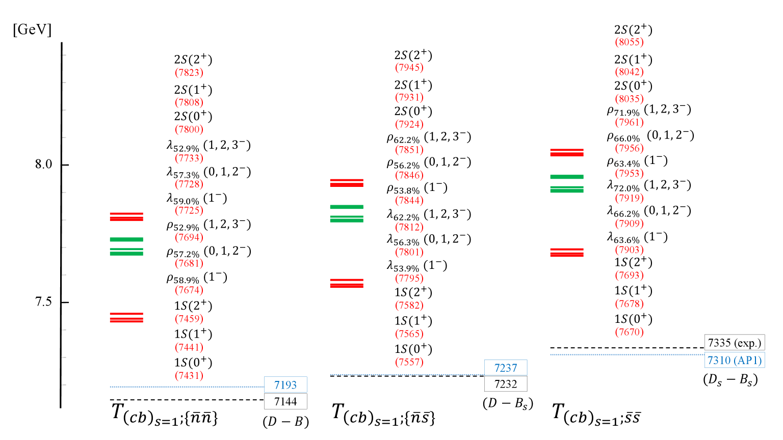
Next we discuss the spectra of the tetraquarks containing the axial-vector antidiquarks. These are illustrated in Figs. 5 and 5, which show the spectrum of $T_{bb}$ and $T_{cc}$ tetraquarks, respectively. The red and green lines stand for the $S$-wave states and the $P$-wave states, respectively. In these figures, the number of strange antiquark is increasing from left to right.

Comparing three spectra in each figure, the masses of these tetraquarks in each state become heavier as the number of the strange antiquark increases, and the mass difference between $T_{QQ;\bar{n}\bar{n}}$ and $T_{QQ;\bar{n}\bar{s}}$ is almost equal to that between $T_{QQ;\bar{n}\bar{s}}$ and $T_{QQ;\bar{s}\bar{s}}$. This behavior comes from the generalized Gell-Mann–Okubo mass formula for the axial-vector diquarks in Eq. (17).

The thresholds shown in Figs. 5 and 5 are for the $0^{+}$ tetraquarks, and are the total mass of two singly heavy mesons with $J^{P}=0^{-}$. Although the $1S$ ground state with $J^{P}=0^{+}$ are the lightest, they are above the thresholds and therefore unstable. Discrepancy between the tetraquark mass and the threshold is even larger for the strange tetraquarks.

About the spin-spin potential terms in the two potential models, Eqs. (20) and (23), both of them are in inverse proportion to the masses of two interacting particles. Therefore, in the heavy-quark limit ($M_{Q_{i}}\rightarrow\infty$), these terms disappear, and the splitted states by the spin-spin interaction become degenerate. This is called the heavy-quark spin (HQS) multiplet which appears frequently in the tetraquark spectra. For example, in Figs. 5 and 5, the $1S$ and $2S$ states of tetraquarks with $J^{P}=0^{+},1^{+}$, and $2^{+}$ have the HQS triplet structure. Comparing these structures in Figs. 5 and 5, we can see that the mass differences for $T_{bb}$ tetraquarks are smaller than those for $T_{cc}$ tetraquarks, which is caused by the bottom quark being heavier than the charm quark.

We here discuss the spectra of $T_{cb}$ tetraquarks. Since two constituent heavy quarks are different from each other, the spin of two heavy quarks, $s$, can take two kinds of values as $s=0$ and $1$. The energy spectra of these tetraquarks are shown in Figs. 7, 7, 9, and 9, classified by the flavor of constituent antidiquarks and the quantum number $s$. Figs. 7 and 7 are the spectra of the strangeness $S=0$ and $+1$ tetraquarks with a flavor $\bm{3}$ antidiquark, respectively. The four colors of lines stand for the types of states and constituent antidiquarks, which is the same as in Figs. 3 and 3. Also, Figs. 9 and 9 are the spectra of the $T_{cb}$ tetraquarks with $s=0$ and $1$, including a flavor $\bar{\bm{6}}$ axial-vector antidiquark, respectively. The two colors of lines stand for the $S$-wave states and the $P$-wave states, which is the same as Figs. 5 and 5.

The spectra of $T_{cb}$ tetraquarks are similar to those of $T_{bb}$ and $T_{cc}$ tetraquarks when the constituent antidiquarks are the same. Although there are less states for the $T_{cb}$ tetraquarks with $s=0$, we can see the effect of chiral effective theory of diquarks: the inverse mass hierarchy of pseudoscalar diquarks and the enhanced mass hierarchy of vector diquarks in Figs. 7 and 7, and the generalized Gell-Mann–Okubo mass formula for the axial-vector diquarks in Figs. 9 and 9.

References

- Aaij et al. (2021a) Roel Aaij et al. (LHCb), “Observation of an exotic narrow doubly charmed tetraquark,” (2021a), arXiv:2109.01038 [hep-ex] .
- Aaij et al. (2021b) Roel Aaij et al. (LHCb), “Study of the doubly charmed tetraquark ,” (2021b), arXiv:2109.01056 [hep-ex] .
- Ader et al. (1982) J. P. Ader, J. M. Richard, and P. Taxil, “Do narrow heavy multiquark states exist?” Phys. Rev. D 25, 2370 (1982).
- Ballot and Richard (1983) J. l. Ballot and J. M. Richard, “Four quark states in additive potentials,” Phys. Lett. B 123, 449–451 (1983).
- Lipkin (1986) Harry J. Lipkin, “A model-independent approach to multiquark bound states,” Phys. Lett. B 172, 242–247 (1986).
- Zouzou et al. (1986) S. Zouzou, B. Silvestre-Brac, C. Gignoux, and J. M. Richard, “Four-quark bound states,” Z. Phys. C 30, 457 (1986).
- Heller and Tjon (1987) L. Heller and J. A. Tjon, “On the Existence of Stable Dimesons,” Phys. Rev. D 35, 969 (1987).
- Carlson et al. (1988) J. Carlson, L. Heller, and J. A. Tjon, “Stability of Dimesons,” Phys. Rev. D 37, 744 (1988).
- Silvestre-Brac and Semay (1993) B. Silvestre-Brac and C. Semay, “Systematics of systems,” Z. Phys. C 57, 273–282 (1993).
- Semay and Silvestre-Brac (1994) C. Semay and B. Silvestre-Brac, “Diquonia and potential models,” Z. Phys. C 61, 271–275 (1994).
- Chow (1995a) Chi-Keung Chow, “Semileptonic decays of heavy tetraquarks,” Phys. Rev. D 51, 3541–3543 (1995a), arXiv:hep-ph/9411221 .
- Chow (1995b) Chi-Keung Chow, “From tetraquarks to hexaquarks: A Systematic study of heavy exotics in the large limit,” Phys. Rev. D 51, 6327–6331 (1995b), arXiv:hep-ph/9412242 .
- Pepin et al. (1997) S. Pepin, F. Stancu, M. Genovese, and J. M. Richard, “Tetraquarks with colour-blind forces in chiral quark models,” Phys. Lett. B 393, 119–123 (1997), arXiv:hep-ph/9609348 .
- Brink and Stancu (1998) D. M. Brink and Fl. Stancu, “Tetraquarks with heavy flavors,” Phys. Rev. D 57, 6778–6787 (1998).
- Gelman and Nussinov (2003) Boris A. Gelman and Shmuel Nussinov, “Does a narrow tetraquark state exist?” Phys. Lett. B 551, 296–304 (2003), arXiv:hep-ph/0209095 .
- Vijande et al. (2004) J. Vijande, F. Fernandez, A. Valcarce, and B. Silvestre-Brac, “Tetraquarks in a chiral constituent quark model,” Eur. Phys. J. A 19, 383 (2004), arXiv:hep-ph/0310007 .
- Janc and Rosina (2004) D. Janc and M. Rosina, “The molecular state,” Few Body Syst. 35, 175–196 (2004), arXiv:hep-ph/0405208 .
- Vijande et al. (2006) J. Vijande, A. Valcarce, and K. Tsushima, “Dynamical study of bf mesons,” Phys. Rev. D 74, 054018 (2006), arXiv:hep-ph/0608316 .
- Ebert et al. (2007) D. Ebert, R. N. Faustov, V. O. Galkin, and W. Lucha, “Masses of tetraquarks with two heavy quarks in the relativistic quark model,” Phys. Rev. D 76, 114015 (2007), arXiv:0706.3853 [hep-ph] .
- Zhang et al. (2008) M. Zhang, H. X. Zhang, and Z. Y. Zhang, “ four-quark bound states in chiral SU(3) quark model,” Commun. Theor. Phys. 50, 437–440 (2008), arXiv:0711.1029 [nucl-th] .
- Vijande et al. (2009) J. Vijande, A. Valcarce, and N. Barnea, “Exotic meson-meson molecules and compact four–quark states,” Phys. Rev. D 79, 074010 (2009), arXiv:0903.2949 [hep-ph] .
- Yang et al. (2009) Youchang Yang, Chengrong Deng, Jialun Ping, and T. Goldman, “-wave state in the constituent quark model,” Phys. Rev. D 80, 114023 (2009).
- Feng et al. (2013) G. Q. Feng, X. H. Guo, and B. S. Zou, “ bound state in the Bethe-Salpeter equation approach,” (2013), arXiv:1309.7813 [hep-ph] .
- Karliner and Rosner (2017) Marek Karliner and Jonathan L. Rosner, “Discovery of doubly-charmed baryon implies a stable () tetraquark,” Phys. Rev. Lett. 119, 202001 (2017), arXiv:1707.07666 [hep-ph] .
- Eichten and Quigg (2017) Estia J. Eichten and Chris Quigg, “Heavy-quark symmetry implies stable heavy tetraquark mesons ,” Phys. Rev. Lett. 119, 202002 (2017), arXiv:1707.09575 [hep-ph] .
- Yan et al. (2018) Xiaojun Yan, Bin Zhong, and Ruilin Zhu, “Doubly charmed tetraquarks in a diquark–antidiquark model,” Int. J. Mod. Phys. A 33, 1850096 (2018), arXiv:1804.06761 [hep-ph] .
- Ali et al. (2018) Ahmed Ali, Qin Qin, and Wei Wang, “Discovery potential of stable and near-threshold doubly heavy tetraquarks at the LHC,” Phys. Lett. B 785, 605–609 (2018), arXiv:1806.09288 [hep-ph] .
- Park et al. (2019) Woosung Park, Sungsik Noh, and Su Houng Lee, “Masses of the doubly heavy tetraquarks in a constituent quark model,” Nucl. Phys. A 983, 1–19 (2019), arXiv:1809.05257 [nucl-th] .
- Deng et al. (2020) Chengrong Deng, Hong Chen, and Jialun Ping, “Systematical investigation on the stability of doubly heavy tetraquark states,” Eur. Phys. J. A 56, 9 (2020), arXiv:1811.06462 [hep-ph] .
- Caramés et al. (2019) Teresa F. Caramés, Javier Vijande, and Alfredo Valcarce, “Exotic four-quark states,” Phys. Rev. D 99, 014006 (2019), arXiv:1812.08991 [hep-ph] .
- Hernández et al. (2020) E. Hernández, J. Vijande, A. Valcarce, and Jean-Marc Richard, “Spectroscopy, lifetime and decay modes of the tetraquark,” Phys. Lett. B 800, 135073 (2020), arXiv:1910.13394 [hep-ph] .
- Yang et al. (2020a) Gang Yang, Jialun Ping, and Jorge Segovia, “Doubly-heavy tetraquarks,” Phys. Rev. D 101, 014001 (2020a), arXiv:1911.00215 [hep-ph] .
- Bedolla et al. (2020) M. A. Bedolla, J. Ferretti, C. D. Roberts, and E. Santopinto, “Spectrum of fully-heavy tetraquarks from a diquark+antidiquark perspective,” Eur. Phys. J. C 80, 1004 (2020), arXiv:1911.00960 [hep-ph] .
- Yu et al. (2020) Meng-Ting Yu, Zhi-Yong Zhou, Dian-Yong Chen, and Zhiguang Xiao, “Possible molecular states in scatterings,” Phys. Rev. D 101, 074027 (2020), arXiv:1912.07348 [hep-ph] .
- Wallbott et al. (2020) Paul C. Wallbott, Gernot Eichmann, and Christian S. Fischer, “Disentangling different structures in heavy-light four-quark states,” Phys. Rev. D 102, 051501 (2020), arXiv:2003.12407 [hep-ph] .
- Tan et al. (2020) Yue Tan, Weichang Lu, and Jialun Ping, “Systematics of in a chiral constituent quark model,” Eur. Phys. J. Plus 135, 716 (2020), arXiv:2004.02106 [hep-ph] .
- Lü et al. (2020) Qi-Fang Lü, Dian-Yong Chen, and Yu-Bing Dong, “Masses of doubly heavy tetraquarks in a relativized quark model,” Phys. Rev. D 102, 034012 (2020), arXiv:2006.08087 [hep-ph] .
- Braaten et al. (2021) Eric Braaten, Li-Ping He, and Abhishek Mohapatra, “Masses of doubly heavy tetraquarks with error bars,” Phys. Rev. D 103, 016001 (2021), arXiv:2006.08650 [hep-ph] .
- Yang et al. (2020b) Gang Yang, Jialun Ping, and Jorge Segovia, “ tetraquarks in the chiral quark model,” Phys. Rev. D 102, 054023 (2020b), arXiv:2007.05190 [hep-ph] .
- Qin et al. (2021) Qin Qin, Yin-Fa Shen, and Fu-Sheng Yu, “Discovery potentials of double-charm tetraquarks,” Chin. Phys. C 45, 103106 (2021), arXiv:2008.08026 [hep-ph] .
- Meng et al. (2021) Q. Meng, E. Hiyama, A. Hosaka, M. Oka, P. Gubler, K. U. Can, T. T. Takahashi, and H. S. Zong, “Stable double-heavy tetraquarks: spectrum and structure,” Phys. Lett. B 814, 136095 (2021), arXiv:2009.14493 [nucl-th] .
- Meng et al. (2022) Qi Meng, Masayasu Harada, Emiko Hiyama, Atsushi Hosaka, and Makoto Oka, “Doubly heavy tetraquark resonant states,” Phys. Lett. B 824, 136800 (2022), arXiv:2106.11868 [hep-ph] .
- Chen (2021) Xiaoyun Chen, “Doubly heavy tetraquark states and ,” (2021), arXiv:2109.02828 [hep-ph] .
- Jin et al. (2021) Yi Jin, Shi-Yuan Li, Yan-Rui Liu, Qin Qin, Zong-Guo Si, and Fu-Sheng Yu, “Color and baryon number fluctuation of preconfinement system in production process and structure,” Phys. Rev. D 104, 114009 (2021), arXiv:2109.05678 [hep-ph] .
- Chen et al. (2021) Kan Chen, Rui Chen, Lu Meng, Bo Wang, and Shi-Lin Zhu, “Systematics of the heavy flavor hadronic molecules,” (2021), arXiv:2109.13057 [hep-ph] .
- Andreev (2021) Oleg Andreev, “On the -Quark Potential in String Models,” (2021), arXiv:2111.14418 [hep-ph] .
- Deng and Zhu (2021) Chengrong Deng and Shi-Lin Zhu, “ and its partners,” (2021), arXiv:2112.12472 [hep-ph] .
- Lee et al. (2008) Su Houng Lee, Shigehiro Yasui, Wei Liu, and Che Ming Ko, “Charmed exotics in Heavy Ion Collisions,” Eur. Phys. J. C 54, 259–265 (2008), arXiv:0707.1747 [hep-ph] .
- Lee and Yasui (2009) Su Houng Lee and Shigehiro Yasui, “Stable multiquark states with heavy quarks in a diquark model,” Eur. Phys. J. C 64, 283–295 (2009), arXiv:0901.2977 [hep-ph] .
- Hyodo et al. (2013) Tetsuo Hyodo, Yan-Rui Liu, Makoto Oka, Kazutaka Sudoh, and Shigehiro Yasui, “Production of doubly charmed tetraquarks with exotic color configurations in electron-positron collisions,” Phys. Lett. B 721, 56–60 (2013), arXiv:1209.6207 [hep-ph] .
- Luo et al. (2017) Si-Qiang Luo, Kan Chen, Xiang Liu, Yan-Rui Liu, and Shi-Lin Zhu, “Exotic tetraquark states with the configuration,” Eur. Phys. J. C 77, 709 (2017), arXiv:1707.01180 [hep-ph] .
- Hyodo et al. (2017) Tetsuo Hyodo, Yan-Rui Liu, Makoto Oka, and Shigehiro Yasui, “Spectroscopy and production of doubly charmed tetraquarks,” (2017), arXiv:1708.05169 [hep-ph] .
- Cheng et al. (2020) Jian-Bo Cheng, Shi-Yuan Li, Yan-Rui Liu, Yu-Nan Liu, Zong-Guo Si, and Tao Yao, “Spectrum and rearrangement decays of tetraquark states with four different flavors,” Phys. Rev. D 101, 114017 (2020), arXiv:2001.05287 [hep-ph] .
- Cheng et al. (2021) Jian-Bo Cheng, Shi-Yuan Li, Yan-Rui Liu, Zong-Guo Si, and Tao Yao, “Double-heavy tetraquark states with heavy diquark-antiquark symmetry,” Chin. Phys. C 45, 043102 (2021), arXiv:2008.00737 [hep-ph] .
- Weng et al. (2022) Xin-Zhen Weng, Wei-Zhen Deng, and Shi-Lin Zhu, “Doubly heavy tetraquarks in an extended chromomagnetic model *,” Chin. Phys. C 46, 013102 (2022), arXiv:2108.07242 [hep-ph] .
- Guo et al. (2022) Tao Guo, Jianing Li, Jiaxing Zhao, and Lianyi He, “Mass spectra of doubly heavy tetraquarks in an improved chromomagnetic interaction model,” Phys. Rev. D 105, 014021 (2022), arXiv:2108.10462 [hep-ph] .
- Navarra et al. (2007) Fernando S. Navarra, Marina Nielsen, and Su Houng Lee, “QCD sum rules study of mesons,” Phys. Lett. B 649, 166–172 (2007), arXiv:hep-ph/0703071 .
- Dias et al. (2011) J. M. Dias, S. Narison, F. S. Navarra, M. Nielsen, and J. M. Richard, “Relation between and from QCD,” Phys. Lett. B 703, 274–280 (2011), arXiv:1105.5630 [hep-ph] .
- Du et al. (2013) Meng-Lin Du, Wei Chen, Xiao-Lin Chen, and Shi-Lin Zhu, “Exotic , and states,” Phys. Rev. D 87, 014003 (2013), arXiv:1209.5134 [hep-ph] .
- Chen et al. (2014) Wei Chen, T. G. Steele, and Shi-Lin Zhu, “Exotic open-flavor , and , tetraquark states,” Phys. Rev. D 89, 054037 (2014), arXiv:1310.8337 [hep-ph] .
- Wang (2018) Zhi-Gang Wang, “Analysis of the axialvector doubly heavy tetraquark states with QCD sum rules,” Acta Phys. Polon. B 49, 1781 (2018), arXiv:1708.04545 [hep-ph] .
- Wang and Yan (2018) Zhi-Gang Wang and Ze-Hui Yan, “Analysis of the scalar, axialvector, vector, tensor doubly charmed tetraquark states with QCD sum rules,” Eur. Phys. J. C 78, 19 (2018), arXiv:1710.02810 [hep-ph] .
- Agaev et al. (2019) S. S. Agaev, K. Azizi, B. Barsbay, and H. Sundu, “Weak decays of the axial-vector tetraquark ,” Phys. Rev. D 99, 033002 (2019), arXiv:1809.07791 [hep-ph] .
- Sundu et al. (2019) H. Sundu, S. S. Agaev, and K. Azizi, “Semileptonic decays of the scalar tetraquark ,” Eur. Phys. J. C 79, 753 (2019), arXiv:1903.05931 [hep-ph] .
- Agaev et al. (2020a) S. S. Agaev, K. Azizi, and H. Sundu, “Double-heavy axial-vector tetraquark ,” Nucl. Phys. B 951, 114890 (2020a), arXiv:1905.07591 [hep-ph] .
- Tang et al. (2020) Liang Tang, Bin-Dong Wan, Kim Maltman, and Cong-Feng Qiao, “Doubly Heavy Tetraquarks in QCD Sum Rules,” Phys. Rev. D 101, 094032 (2020), arXiv:1911.10951 [hep-ph] .
- Agaev et al. (2020b) S. S. Agaev, K. Azizi, B. Barsbay, and H. Sundu, “Heavy exotic scalar meson ,” Phys. Rev. D 101, 094026 (2020b), arXiv:1912.07656 [hep-ph] .
- Agaev et al. (2020c) S. S. Agaev, K. Azizi, B. Barsbay, and H. Sundu, “Stable scalar tetraquark ,” Eur. Phys. J. A 56, 177 (2020c), arXiv:2001.01446 [hep-ph] .
- Wang and Chen (2020) Qi-Nan Wang and Wei Chen, “Fully open-flavor tetraquark states and with ,” Eur. Phys. J. C 80, 389 (2020), arXiv:2002.04243 [hep-ph] .
- Agaev et al. (2021a) S. S. Agaev, K. Azizi, B. Barsbay, and H. Sundu, “A family of double-beauty tetraquarks: Axial-vector state ,” Chin. Phys. C 45, 013105 (2021a), arXiv:2002.04553 [hep-ph] .
- Agaev et al. (2021b) S. S. Agaev, K. Azizi, B. Barsbay, and H. Sundu, “Semileptonic and nonleptonic decays of the axial-vector tetraquark ,” Eur. Phys. J. A 57, 106 (2021b), arXiv:2008.02049 [hep-ph] .
- Agaev et al. (2022) S. S. Agaev, K. Azizi, and H. Sundu, “Newly observed exotic doubly charmed meson ,” Nucl. Phys. B 975, 115650 (2022), arXiv:2108.00188 [hep-ph] .
- Azizi and Özdem (2021) K. Azizi and U. Özdem, “Magnetic dipole moments of the and tetraquark states,” Phys. Rev. D 104, 114002 (2021), arXiv:2109.02390 [hep-ph] .
- Aliev et al. (2021) T. M. Aliev, S. Bilmis, and M. Savci, “Determination of the spectroscopic parameters of beauty-partners of from QCD,” (2021), arXiv:2111.01081 [hep-ph] .
- Özdem (2022) Ulaş Özdem, “Magnetic moments of the doubly charged axial-vector states,” Phys. Rev. D 105, 054019 (2022), arXiv:2112.10402 [hep-ph] .
- Bilmiş (2021) Selçuk Bilmiş, “Mixing angles between the tetraquark states with two heavy quarks within QCD sum rules,” Turk. J. Phys. 45, 390–399 (2021), arXiv:2201.06109 [hep-ph] .
- Detmold et al. (2007) William Detmold, Kostas Orginos, and Martin J. Savage, “ Potentials in Quenched Lattice QCD,” Phys. Rev. D 76, 114503 (2007), arXiv:hep-lat/0703009 .
- Wagner (2010) Marc Wagner (ETM, Y), “Forces between static-light mesons,” PoS LATTICE2010, 162 (2010), arXiv:1008.1538 [hep-lat] .
- Bali and Hetzenegger (2010) Gunnar Bali and Martin Hetzenegger (QCDSF), “Static-light meson-meson potentials,” PoS LATTICE2010, 142 (2010), arXiv:1011.0571 [hep-lat] .
- Bicudo and Wagner (2013) Pedro Bicudo and Marc Wagner (European Twisted Mass), “Lattice QCD signal for a bottom-bottom tetraquark,” Phys. Rev. D 87, 114511 (2013), arXiv:1209.6274 [hep-ph] .
- Brown and Orginos (2012) Zachary S. Brown and Kostas Orginos, “Tetraquark bound states in the heavy-light heavy-light system,” Phys. Rev. D 86, 114506 (2012), arXiv:1210.1953 [hep-lat] .
- Ikeda et al. (2014) Yoichi Ikeda, Bruno Charron, Sinya Aoki, Takumi Doi, Tetsuo Hatsuda, Takashi Inoue, Noriyoshi Ishii, Keiko Murano, Hidekatsu Nemura, and Kenji Sasaki, “Charmed tetraquarks and from dynamical lattice QCD simulations,” Phys. Lett. B 729, 85–90 (2014), arXiv:1311.6214 [hep-lat] .
- Bicudo et al. (2015) Pedro Bicudo, Krzysztof Cichy, Antje Peters, Björn Wagenbach, and Marc Wagner, “Evidence for the existence of and the non-existence of and tetraquarks from lattice QCD,” Phys. Rev. D 92, 014507 (2015), arXiv:1505.00613 [hep-lat] .
- Bicudo et al. (2016) Pedro Bicudo, Krzysztof Cichy, Antje Peters, and Marc Wagner, “ interactions with static bottom quarks from Lattice QCD,” Phys. Rev. D 93, 034501 (2016), arXiv:1510.03441 [hep-lat] .
- Francis et al. (2017) Anthony Francis, Renwick J. Hudspith, Randy Lewis, and Kim Maltman, “Lattice Prediction for Deeply Bound Doubly Heavy Tetraquarks,” Phys. Rev. Lett. 118, 142001 (2017), arXiv:1607.05214 [hep-lat] .
- Bicudo et al. (2017a) Pedro Bicudo, Jonas Scheunert, and Marc Wagner, “Including heavy spin effects in the prediction of a tetraquark with lattice QCD potentials,” Phys. Rev. D 95, 034502 (2017a), arXiv:1612.02758 [hep-lat] .
- Bicudo et al. (2017b) Pedro Bicudo, Marco Cardoso, Antje Peters, Martin Pflaumer, and Marc Wagner, “ tetraquark resonances with lattice QCD potentials and the Born-Oppenheimer approximation,” Phys. Rev. D 96, 054510 (2017b), arXiv:1704.02383 [hep-lat] .
- Francis et al. (2019) Anthony Francis, Renwick J. Hudspith, Randy Lewis, and Kim Maltman, “Evidence for charm-bottom tetraquarks and the mass dependence of heavy-light tetraquark states from lattice QCD,” Phys. Rev. D 99, 054505 (2019), arXiv:1810.10550 [hep-lat] .
- Junnarkar et al. (2019) Parikshit Junnarkar, Nilmani Mathur, and M. Padmanath, “Study of doubly heavy tetraquarks in Lattice QCD,” Phys. Rev. D 99, 034507 (2019), arXiv:1810.12285 [hep-lat] .
- Leskovec et al. (2019) Luka Leskovec, Stefan Meinel, Martin Pflaumer, and Marc Wagner, “Lattice QCD investigation of a doubly-bottom tetraquark with quantum numbers ,” Phys. Rev. D 100, 014503 (2019), arXiv:1904.04197 [hep-lat] .
- Hudspith et al. (2020) R. J. Hudspith, B. Colquhoun, A. Francis, R. Lewis, and K. Maltman, “A lattice investigation of exotic tetraquark channels,” Phys. Rev. D 102, 114506 (2020), arXiv:2006.14294 [hep-lat] .
- Mohanta and Basak (2020) Protick Mohanta and Subhasish Basak, “Construction of tetraquark states on lattice with NRQCD bottom and HISQ up and down quarks,” Phys. Rev. D 102, 094516 (2020), arXiv:2008.11146 [hep-lat] .
- Bicudo et al. (2021) Pedro Bicudo, Antje Peters, Sebastian Velten, and Marc Wagner, “Importance of meson-meson and of diquark-antidiquark creation operators for a tetraquark,” Phys. Rev. D 103, 114506 (2021), arXiv:2101.00723 [hep-lat] .
- Padmanath and Mathur (2021) M. Padmanath and Nilmani Mathur, “four-quark states from Lattice QCD,” in 38th International Symposium on Lattice Field Theory (2021) arXiv:2111.01147 [hep-lat] .
- Harada et al. (2020) Masayasu Harada, Yan-Rui Liu, Makoto Oka, and Kei Suzuki, “Chiral effective theory of diquarks and the anomaly,” Phys. Rev. D 101, 054038 (2020), arXiv:1912.09659 [hep-ph] .
- Kim et al. (2020) Yonghee Kim, Emiko Hiyama, Makoto Oka, and Kei Suzuki, “Spectrum of singly heavy baryons from a chiral effective theory of diquarks,” Phys. Rev. D 102, 014004 (2020), arXiv:2003.03525 [hep-ph] .
- Kim et al. (2021) Yonghee Kim, Yan-Rui Liu, Makoto Oka, and Kei Suzuki, “Heavy baryon spectrum with chiral multiplets of scalar and vector diquarks,” Phys. Rev. D 104, 054012 (2021), arXiv:2105.09087 [hep-ph] .
- ’t Hooft (1976) Gerard ’t Hooft, “Computation of the Quantum Effects Due to a Four-Dimensional Pseudoparticle,” Phys. Rev. D 14, 3432–3450 (1976), [Erratum: Phys.Rev.D 18, 2199 (1978)].
- ’t Hooft (1986) Gerard ’t Hooft, “How Instantons Solve the Problem,” Phys. Rept. 142, 357–387 (1986).
- Gell-Mann (1962) M. Gell-Mann, “Symmetries of baryons and mesons,” Phys. Rev. 125, 1067–1084 (1962).
- Okubo (1962) Susumu Okubo, “Note on unitary symmetry in strong interactions,” Prog. Theor. Phys. 27, 949–966 (1962).
- Silvestre-Brac (1996) B. Silvestre-Brac, “Spectrum and static properties of heavy baryons,” Few Body Syst. 20, 1 (1996).
- Zyla et al. (2020) P.A. Zyla et al. (Particle Data Group), “Review of Particle Physics,” PTEP 2020, 083C01 (2020).
- Yoshida et al. (2015) Tetsuya Yoshida, Emiko Hiyama, Atsushi Hosaka, Makoto Oka, and Katsunori Sadato, “Spectrum of heavy baryons in the quark model,” Phys. Rev. D92, 114029 (2015), arXiv:1510.01067 [hep-ph] .
- Kamimura (1988) M. Kamimura, “Nonadiabatic coupled-rearrangement-channel approach to muonic molecules,” Phys. Rev. A38, 621 (1988).
- Hiyama et al. (2003) E. Hiyama, Y. Kino, and M. Kamimura, “Gaussian expansion method for few-body systems,” Prog. Part. Nucl. Phys. 51, 223 (2003).
- Kumakawa and Jido (2017) Kento Kumakawa and Daisuke Jido, “Excitation energy spectra of the and baryons in a finite-size diquark model,” PTEP 2017, 123D01 (2017), arXiv:1708.02012 [nucl-th] .
- Kumakawa and Jido (2021) Kento Kumakawa and Daisuke Jido, “Excitation spectra of heavy baryons in diquark models,” (2021), arXiv:2107.11950 [hep-ph] .