Doubly heavy tetraquarks in the chiral quark soliton model
Abstract
The chiral quark soliton model has been successfully applied to describe the heavy baryon spectrum, both for charm and bottom, leading to the conclusion that the heavy quark has no effect on the soliton. This suggests that replacing a heavy quark by a heavy antidiquark in color triplet should give a viable description of heavy tetraquarks. We follow this strategy to compute tetraquark masses. To estimate heavy diquark masses we use the Cornell potential with appropriately rescaled parameters. The lightest charm tetraquark is 70 MeV above the threshold. On the contrary, both nonstrange and strange bottom tetraquarks are bound by approximately 140 and 60 MeV, respectively.
I Introduction
Recent discovery of a doubly charmed tetraquark with a mass of MeV, approximately keV below the threshold, by the LHCb Collaboration [1, 2] triggered a number of theoretical studies of exotic heavy-light states. A comprehensive review of multiquark states, both experimental and theoretical, before discovery can be found in Ref. [3] and more recently after the discovery of in Ref. [4] and references therein. The up to date compilation of theoretical results is best illustrated in Fig. 42 of Ref. [4].
The existence of heavy tetraquarks has been anticipated theoretically already many yers ago [5]. In 1993, Manohar and Wise [6] showed using heavy quark symmetry [7] that tetraquarks are bound in the limit (see also [8, 9]). This has been also pointed out more recently in Ref. [10]. To the best of our knowledge, the first estimate of a doubly heavy tetraquark mass is from Lipkin in 1986 [11] (although the fourfold heavy tetraquarks were discussed even earlier in 1982 [12]). We have reviewed the variational approach of Ref. [11] in Ref. [13] adding new information coming from the discovery of [14] and showing that the upper bound on a mass is approximately 60 MeV above the threshold. On the contrary, the bound on a mass was 224 MeV below the threshold. In the same paper, we advocated the possibility of using the chiral quark soliton model (QSM) to estimate the mass.
A mean field description of heavy baryons as a light quark-soliton and a heavy quark has been introduced and developed in Refs. [15, 16, 17, 18]. This approach is a modification of the QSM used previously to describe light baryons (see [19] and Refs. [20, 21, 22] for review) where the soliton is constructed from light quarks. To describe heavy baryons one has to remove one light quark from the valence level and add a heavy quark instead. In the large limit this replacement hardly changes the mean fields of the soliton.
Support for such a treatment can be inferred from Ref. [23] where the authors studied soliton behavior in the limit where the current quark masses are . Although such a limit may at first sight be in contradiction with the chiral symmetry, which is the main theoretical basis of the model, it gave very good phenomenological results when compared to lattice data at finite . At sufficiently large , the soliton ceases to exist, and the correct heavy quark limit is achieved.
In the QSM, the soliton mass is given as a sum over the energies of the valence quarks and the sea quark energies computed with respect to the vacuum and appropriately regularized [23],
| (1) |
In the present context, Eq. (1) takes the following form:
| (2) | ||||
As has been argued in Ref. [23], for large , the sum over the sea quarks in the second line of Eq. (2) vanishes, and . One copy of the soliton ceases to exist; however, the remaining quarks still form a stable soliton.
Such a soliton does not carry any quantum numbers except for the baryon number resulting from the valence quarks. Spin and isospin appear when the soliton rotations in space and flavor are quantized. This procedure results in a collective Hamiltonian analogous to the one of a quantum mechanical symmetric top; however, due to the Wess-Zumino-Witten term [24, 25], the allowed Hilbert space is truncated to the representations that contain states of hypercharge . For (1), these are octet and decuplet of ground state baryons. For (2), we have antitriplet of spin 0 and sextet of spin 1. It is therefore convenient to label heavy quark baryons (and tetraquarks as well) by the SU(3)flavor representation of the light subsystem.
From this perspective, the soliton is reminiscent of a diquark, and the quantization rule selects SU(3)flavor representations identical as the ones of the quark model. Given the success of the QSM in reproducing the data [15, 16, 17, 18], we propose here to use the same strategy to describe the doubly heavy tetraquarks replacing heavy quark by a heavy (anti)diquark .
We observe that two heavy quarks of the same flavor (say or ) can form a color antitriplet (antisymmetric in color) provided they are symmetric in spin [26]. Therefore, they form a tight object of spin 1. Hence, two heavy antiquarks are in color and spin 1, behaving as a spin 1 heavy quark. A tetraquark can be therefore viewed as being composed of a heavy (anti)diquark of spin 1 and a ()-quark soliton.111In what follows, we use term diquark referring both to and states.
There are three main lessons that we have learned from our previous studies of heavy baryons [15, 16, 17, 18]:
-
•
the soliton properties do not depend on the mass of the heavy quark,
-
•
neither do they depend on the spin coupling between a soliton and a heavy quark,
-
•
hyperfine splittings scale like .
This is discussed in detail in Sec. II.
Therefore, a very simple and predictive picture of a soliton + heavy object (that is in color) bound state emerges, where the mass is simply given as a sum of the soliton mass (including and rotational splittings), mass of a heavy object (quark or a diquark), and the hyperfine splitting. This picture is very reminiscent to the one of Ref. [10]. Mass formulas for such states are therefore identical to the ones of heavy baryons, with some modification due to the spin 1 character of the heavy diquark; this is elaborated on in detail in Sec. III. So the main problem is to estimate the diquark mass. Here, we propose to use the Cornell potential as described later in Sec. IV.
II Chiral Quark Soliton Model for Baryons
Let us first recall how baryon masses are calculated in the present model. We quantize the soliton as if it were constructed from rather than light quarks. Then, in the chiral limit the soliton energy is given as
| (3) |
Here, is a classical soliton mass, denote moments of inertia, is the SU(3)flavor Casimir, and corresponds to spin. In our case and the allowed SU(3) representations correspond to with spin and with spin [15].
SU(3) splittings are given by the operator
| (4) |
where constants , and can be expressed through generalized moments of inertia (see e.g. Eq. (4) in Ref [15]) and can be computed ab initio in some specific versions of the model. In the most simple case with the pseudoscalar fields only, the numerical values can be found e.g. in Ref. [27], and in the context of heavy baryons in Ref. [28]. In both cases they lead to reasonable phenomenology. However, in reality one should take into account all possible chiral fields: scalar, pseudoscalar, vector, axial and tensor [29] for which full numerical analysis has not been performed. Here, the explicit forms of , and are not needed as we treat them as free parameters.
Heavy baryon masses are calculated by adding the mass of the heavy quark to the soliton mass and by taking into account the hyperfine splitting given by the following Hamiltonian:
| (5) |
where and stand for the soliton and heavy quark spin, respectively. We have assumed here that the possible dependence of , due to the presence of the wave function squared in (5), can be ignored. Since the spin of the representation is zero, there is no hyperfine splitting in this case. In the case of we have two sets of heavy baryons with spins and This pattern is seen in the experimental data [30].
Mass formulas for heavy baryons read therefore as follows [13]:
| (9) |
Here splitting parameters and are known functions of parameters , and (see Eq. (9) in Ref. [15]), and stands for a hypercharge of a given baryon.
Let us examine the consequences of the mass formulas (9). First of all, as has been already observed in [15], Eqs. (9) admit one parameter independent sum rule in the sextet
| (10) |
which for charm is satisfied at the level MeV. We use (10) to estimate MeV when we compute average sextet masses in the sector.
To get rid of the hyperfine splittings, we average out spin dependence in sextets by defining
| (11) |
Average masses and masses in triplets should be equally spaced with . independently of the heavy quark.222We neglect small isospin violation. For we have (in MeV)
| (12) |
which is satisfied with 2 % accuracy. In the case of , we have more relations (in MeV),
| (13) | ||||
| (14) |
which are satisfied with 4 % accuracy.333Note that for numerical analysis in the present paper, we have used most recent version of PDG [30], and therefore, there are small numerical differences with respect to Ref. [15].
We can also form differences of average multiplet masses between the and sectors to compute the heavy quark mass difference (in MeV),
| (15) |
Furthermore, we can extract the hyperfine splitting parameter testing our assumptions concerning the Hamiltonian (5),
| (16) | ||||
| (17) |
(in MeV). From these estimates, we get
| (18) |
with the average value of . The PDG values of the heavy quark masses lead to where both masses are evaluated at the renormalization point [30]. Of course, heavy quark masses in the effective models, like the one considered in this paper, may differ from the QCD masses. It is therefore encouraging that we get a mass ratio close to the ratio of the QCD masses. Nevertheless, quark masses extracted from Eqs. (15) and (18),
| (19) |
are a bit higher (especially for ) than those quoted by PDG [30]. For , we get MeV and MeV, which are still lower than the effective values used, e.g., in Ref. [31].
Finally, to test heavy quark dependence of the mass formulas (9), we can compute the nonstrange moment of inertia from the sextet- average mass differences,
| (20) |
in MeV. We see that indeed heavy quark masses cancel with very high precision. This, together with Eq. (15), suggests that possible nonlinear in binding effects are very small if not vanishing. We can therefore safely assume that formulas (15) are valid for any heavy object replacing . We pursue this possibility in the next section.
III Chiral Quark Soliton Model for Tetraquarks
In the present case, instead of a heavy quark, we add to the soliton a heavy diquark of spin 1. Assuming that the soliton is not changed by this replacement we arrive at the following mass formulas for tetraquarks:
| (21) |
where is a spin factor arising from the fact that both the sextet soliton and the diquark have spin 1:
| (22) |
Here is a heavy baryon mass in SU(3)flavor and is a spin averaged mass of a sextet baryon (11).
Sextet splittings satisfy the following relation
| (23) | |||||
Before proceeding to numerical calculations let us discuss strong decay thresholds. Since the ground state tetraquarks have , they can decay to or . The corresponding thresholds are listed in the second rows of Tables 1 and 2 for nonstrange and strange tetraquarks, respectively. In the latter case, and thresholds are lighter than or .
In the case of the sextet tetraquarks, we have three families of spin , 1, and of nonstrange, strange and doubly strange tetraquarks. Pertinent thresholds (averaged over isospin) are listed in Tables 1–3.
| Channel | Thresholds [MeV] | |
|---|---|---|
| 3736.1 10558.9 | ||
| 3877.2 10604.2 | ||
| 4018.3 10649.4 |
| Channel | Thresholds [MeV] | |
|---|---|---|
| 3836.4 10646.4 | ||
| 3977.5 10691.6 | ||
| 4121.3 10740.1 |
| Channel | Thresholds [MeV] | |
|---|---|---|
| 3936.7 10733.8 | ||
| 4080.6 10782.3 | ||
| 4224.4 10830.8 |
Mass formulas (22) relate tetraquark masses directly to heavy baryon masses and therefore are fairly model independent. They are analogous to the masses given in Eq.(1) of Ref. [10]. The spin part has been discussed in [10] and in [32]; however, the hyperfine coupling has not been specified. Here, we know the value of (17), so in order to estimate tetraquark masses, we only need heavy diquark mass for in the range (19).
IV Heavy Diquark Mass
The main problem in predicting heavy tetraquark masses in the present model is to have a reliable estimate of the heavy diquark mass, as it is beyond the large effective theory that we have used for the light sector. To this end, we propose to apply a nonrelativistic Schrödinger equation with the Cornell potential [33]
| (24) |
with , which has been successfully used to describe heavy spectra (see, e.g., Ref. [34]).
There are two practical reasons to use the Cornell potential in the present context. The first one is that in order to compute (or ) masses one has to rescale model parameters by a factor of 2. This follows from the fact that the color charge is factor 2 smaller when quark color charges are in an (anti)triplet than in a singlet (see, e.g., Table III in Ref. [31]). As this is quite obvious for the Coulomb term, lattice calculations suggest the same behavior of the confining part [35]. Also the chromomagnetic spin interaction, which we neglect in the following, scales in the same way.
The second reason is that the Coulomb part in potential (24) can be in fact considered as a perturbation to the linear potential, for which solutions in terms of the Airy functions are known semianalytically. We have checked that it is enough to consider only the first order perturbation theory.
We are interested in the states only, so we put in the pertinent Schrödinger equation. The reduced mass of the equal mass system entering the Schrödinger equation is . So we are looking for a solution in terms of a function defined as follows:
| (25) |
It is convenient to introduce a dimensionless variable ,
| (26) |
and rescaled dimensionless parameters and ,
| (27) |
With these substitutions, the Schrödinger equation takes a very simple form,
| (28) |
For , Eq. (28) reduces to the Airy equation, and the unperturbed energies are given in terms of the zeros of the Airy function . This follows from the boundary condition . Therefore, we have energy quantization,
| (29) |
Note that these zeros are negative, so the energy is positive. The normalized solution is
| (30) |
First order perturbative correction is linear in , so the full energy reads
| (31) |
We need energies for two first levels only, for which and . Masses of the states read
| (32) |
where we have introduced two new parameters,
| (33) |
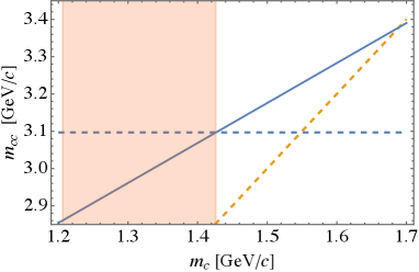
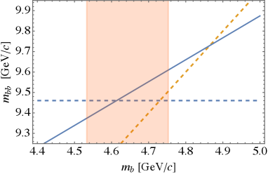
For a given from the range covering (19), we have computed parameters and from the two lowest states.444Parameters and must be positive. It turns out that there are no such solutions for too low . Since we need to estimate the mass of a spin 1 diquark, we have chosen as inputs and for charm and and for bottom. We have checked that the original parameters and obtained that way are in qualitative agreement with numerical results of Ref. [34].
Having and fixed, we can easily compute diquark masses in color (anti)triplet by rescaling and , leading to and . It is important to realize that the two terms in Eq. (32) scale differently with this change of parameters. The confining positive part is reduced by a factor while the Coulomb negative part is reduced by . This delicate balance can make the diquark mass higher than the ground state. This happens, however, only at sufficiently high where the first order perturbation theory breaks down.
The diquark masses for charm and bottom are plotted in Fig. 1. One can see that at sufficiently large mass the Coulomb term becomes equal to the confining term, and the diquark mass becomes lighter than signaling the break down of the first order perturbation theory. However, in the range of model masses (19), the linear confining term dominates, and the first order perturbation theory is sufficient. In Ref. [13], we have naively approximated , whereas for the Cornell potential, we get in the mass range (19). This seemingly small difference led to the overbinding observed in [13].
It is of course legitimate to ask how the diquark masses depend on the potential that one chooses do describe heavy quark dynamics. One could try, for example, a harmonic oscillator potential, which for MeV and MeV reproduces masses of and . After rescaling (which is a naive implementation of the rescaling valid for the Cornell potential), one obtains MeV, 60 MeV below the mass following from the Cornell potential for MeV. Nevertheless, as we shall shortly see, this reduction does not lead to a bound tetraquark state.
V Tetraquark Masses
V.1 Antitriplet masses
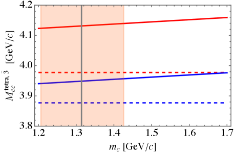
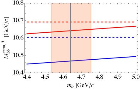
It is now straightforward to compute predictions for the tetraquarks in flavor with the help of Eqs.(21) and the numerical results for the diquark masses from the previous section. The results are plotted in Fig. 2 and listed in Table 4. We can see that charm tetraquark masses are above the threshold, while in the case of bottom we see rather deeply bound states both for nonstrange and strange tetraquarks. The lightest nonstrange charm tetraquark is approximately 70 MeV above the threshold, so even the harmonic oscillator model for the heavy diquark would not lead to binding. Our results are in a very good agreement with predictions of Ref. [10], although up to 30 MeV lower.
| Charm | Bottom | |
|---|---|---|
| 1.31 | 4.64 | |
| 3.95 | 10.47 | |
| 4.13 | 10.64 |
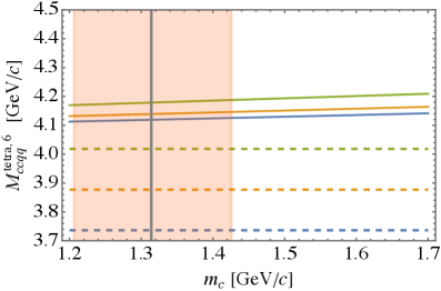
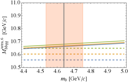
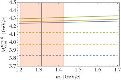
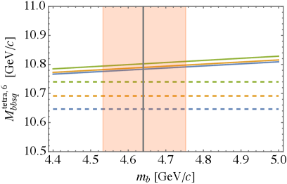
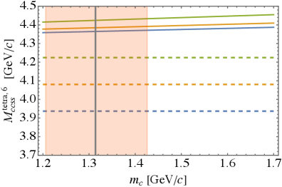
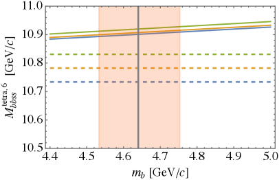
V.2 Sextet masses
The only difference between the antitriplet masses and sextet masses is the presence of the hyperfine splitting. Interestingly, from (23), we expect for charm MeV, as in the range (19) is approximately . On the contrary, hyperfine splitting MeV is 7 times larger (and similarly in the sector). So in fact different spin states in the sextet are almost degenerate. We see this clearly in Fig. 3 where we plot predictions for the sextet tetraquark masses (solid lines) and the pertinent thresholds (dashed lines). Different colors correspond to spin. The only possible candidate for a bound state, given the accuracy of the present model, is a nonstrange bottom tetraquark of spin 2, which is only MeV above the threshold. Numerical values can be found in Table 5.
VI Summary and Conclusions
Motivated by the success of the chiral quark soliton model in describing the heavy baryon spectra, we have constructed mass formulas for heavy tetraquarks with two heavy quarks of the same flavor. We first discussed baryon phenomenology to conclude that the properties of the light sector do not depend on the heavy quark properties. This is quite expected on the grounds of heavy quark symmetry. It is therefore legitimate to replace heavy quark in color by a heavy anti-diquark, that differs from by mass and spin. Mass formulas (9) relate tetraquark masses to the masses of heavy baryons, and the only model parameter borrowed from the baryon phenomenology is the hyperfine splitting parameter (17) . In this sense, our approach, although derived from the QSM, is fairly model independent. This is why formulas (9) are identical to the ones derived in the heavy quark limit from QCD in Ref. [10].
| Charm | Bottom | |||||
|---|---|---|---|---|---|---|
| 1.31 | 4.64 | |||||
| 0 | 1 | 2 | 0 | 1 | 2 | |
| 4.12 | 4.14 | 4.18 | 10.66 | 10.67 | 10.68 | |
| 4.25 | 4.27 | 4.31 | 10.78 | 10.79 | 10.80 | |
| 4.37 | 4.38 | 4.42 | 10.90 | 10.91 | 10.92 | |
The only unknown ingredient of the present approach is the heavy diquark mass. To this end, we have used the Cornell potential, first to fit potential parameters to reproduce lowest spin 1 onia, both in charm and bottom sectors, and then, after rescaling these parameters, to compute the spin 1 diquark masses. We find that only bottom tetraquarks in flavor antitriplet are bound, while the charm ones are above the threshold. This is true also in the case when the structure of a heavy diquark can be resolved by the light quarks and repulsive color channel is included [36].
Numerical results presented in Tables 4 and 5 are in a very good agreement with the results of Ref. [10] where all necessary parameters have been extracted from data, including the mass of [14]. No model calculations have been performed in Ref. [10], and in turn, we did not use any input from doubly charmed . This is a strong argument in favor of our approach to the heavy diquark mass.
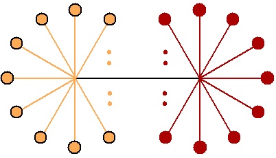
It is interesting to observe that our model has a completely different counting than typical models discussed, e.g., in Refs. [26] or [36], where tetraquarks are composed from four quarks for any . In our case, the soliton for large belongs to a color representation corresponding to an antisymmetric product on quarks. This is because we have to take one light quark from the soliton and add one heavy quark to construct a heavy baryon. For , this is . In order to construct a tetraquark, we need to put heavy antiquarks in a complex conjugate representation corresponding to antisymmetrized antiquarks. For , this is . So for arbitrary , our tetraquark consits of light quarks and heavy antiquarks, see Fig. 4. Such a configuration has been briefly discussed in Ref. [26]. A system composed of heavy (anti)quarks is amenable to semiclassical treatment. It would be interesting to pursue this possibility in constructing a model for a diquark.
Finally, we have to confront the LHCb tetraquark [1, 2] which is just below the threshold. Here, two possibilities exist. Either our model is not accurate enough to deal with dynamics which gives binding energies of the order of hundreds keV, or the LHCb tetraquark corresponds to a different configuration that is out of reach for the soliton models. Obviously, charm quark mass is far from infinity and corrections might finally lower our predictions. In the present approach, however, we have no systematic scheme that would allow one to include such effects. Also the diquark model can be responsible for overshooting the physical mass. Nevertheless, given the very good accuracy of the QSM predictions for heavy baryon masses and very good agreement with the phenomenological analysis of Ref. [10], one is perhaps more inclined towards the second possibility. Indeed, the LHCb [2] estimated the size of to be of the order of fm, significantly larger than the typical size of heavy flavor hadrons. This suggests a molecular structure of [37, 38].
In order to compute the space (or momentum) structure of tetraquarks in the present model, one should resort to a dynamical description of the soliton in terms of quark degrees of freedom. Some studies in this direction within QSM have been undertaken in the case of singly heavy baryons. In Ref. [39] electromagnetic form factors and in Refs. [40, 41] gravitational form factors have been studied. It follows that heavy baryons are more compact than the proton. That conclusion should also apply to the present case, as the heavy quark or diquark is treated here merely as a static color source. The internal structure of heavy tetraquarks certainly deserves detailed studies, it is, however, beyond scope of the present paper.
Acknowledgements
This research has been supported by the Polish National Science Centre Grants No. 2017/27/B/ST2/01314 and No. 2018/31/B/ST2/01022. The author thanks the Institute for Nuclear Theory at the University of Washington for its kind hospitality, stimulating research environment and partial support by the INT’s U.S. Department of Energy Grant No. DE-FG02-00ER41132.
References
- [1] R. Aaij et al. [LHCb], Nature Phys. 18, no.7, 751-754 (2022) doi:10.1038/s41567-022-01614-y [arXiv:2109.01038 [hep-ex]].
- [2] R. Aaij et al. [LHCb], Nature Commun. 13, no.1, 3351 (2022) doi:10.1038/s41467-022-30206-w [arXiv:2109.01056 [hep-ex]].
- [3] M. Karliner, J. L. Rosner and T. Skwarnicki, Ann. Rev. Nucl. Part. Sci. 68, 17-44 (2018) doi:10.1146/annurev-nucl-101917-020902 [arXiv:1711.10626 [hep-ph]].
- [4] H. X. Chen, W. Chen, X. Liu, Y. R. Liu and S. L. Zhu, [arXiv:2204.02649 [hep-ph]].
- [5] J. Carlson, L. Heller and J. A. Tjon, Phys. Rev. D 37, 744 (1988) doi:10.1103/PhysRevD.37.744
- [6] A. V. Manohar and M. B. Wise, Nucl. Phys. B 399, 17 (1993).
- [7] N. Isgur and M. B. Wise, Phys. Rev. Lett. 66, 1130-1133 (1991) doi:10.1103/PhysRevLett.66.1130
- [8] T. D. Cohen and P. M. Hohler, Phys. Rev. D 74, 094003 (2006).
- [9] Y. Cai and T. Cohen, Eur. Phys. J. A 55, no.11, 206 (2019) doi:10.1140/epja/i2019-12906-0 [arXiv:1901.05473 [hep-ph]].
- [10] E. J. Eichten and C. Quigg, Phys. Rev. Lett. 119, no.20, 202002 (2017) doi:10.1103/PhysRevLett.119.202002 [arXiv:1707.09575 [hep-ph]].
- [11] H. J. Lipkin, Phys. Lett. B 172, 242 (1986).
- [12] J. P. Ader, J. M. Richard and P. Taxil, Phys. Rev. D 25, 2370 (1982).
- [13] M. Praszałowicz, Acta Phys. Polon. Supp. 13, 103-108 (2020) doi:10.5506/APhysPolBSupp.13.103 [arXiv:1904.02676 [hep-ph]].
- [14] R. Aaij et al. [LHCb], Phys. Rev. Lett. 119, no.11, 112001 (2017) doi:10.1103/PhysRevLett.119.112001 [arXiv:1707.01621 [hep-ex]].
- [15] G. S. Yang, H. C. Kim, M. V. Polyakov and M. Praszałowicz, Phys. Rev. D 94, 071502 (2016) doi:10.1103/PhysRevD.94.071502 [arXiv:1607.07089 [hep-ph]].
- [16] H. C. Kim, M. V. Polyakov and M. Praszałowicz, Phys. Rev. D 96, no.1, 014009 (2017) doi:10.1103/PhysRevD.96.014009 [arXiv:1704.04082 [hep-ph]].
- [17] H. C. Kim, M. V. Polyakov, M. Praszałowicz and G. S. Yang, Phys. Rev. D 96, no.9, 094021 (2017) [erratum: Phys. Rev. D 97, no.3, 039901 (2018)] doi:10.1103/PhysRevD.96.094021 [arXiv:1709.04927 [hep-ph]].
- [18] M. V. Polyakov and M. Praszałowicz, Phys. Rev. D 105, 094004 (2022) doi:10.1103/PhysRevD.105.094004 [arXiv:2201.07293 [hep-ph]].
- [19] D. Diakonov, V. Y. Petrov and P. V. Pobylitsa, Nucl. Phys. B 306 (1988) 809.
- [20] C. V. Christov, A. Blotz, H. C. Kim, P. Pobylitsa, T. Watabe, T. Meissner, E. Ruiz Arriola and K. Goeke, Prog. Part. Nucl. Phys. 37 (1996) 91.
- [21] R. Alkofer, H. Reinhardt and H. Weigel, Phys. Rept. 265 (1996) 139.
- [22] V. Petrov, Acta Phys. Polon. B 47 (2016) 59.
- [23] K. Goeke, J. Ossmann, P. Schweitzer and A. Silva, Eur. Phys. J. A 27, 77-90 (2006), doi:10.1140/epja/i2005-10229-5, [arXiv:hep-lat/0505010 [hep-lat]].
- [24] E. Witten, Nucl. Phys. B 223 (1983) 422, and 223 (1983) 433.
- [25] J. Wess and B. Zumino, Phys. Lett. B 37, 95-97 (1971) doi:10.1016/0370-2693(71)90582-X
- [26] B. A. Gelman and S. Nussinov, Phys. Lett. B 551, 296-304 (2003) doi:10.1016/S0370-2693(02)03069-1 [arXiv:hep-ph/0209095 [hep-ph]].
- [27] A. Blotz, D. Diakonov, K. Goeke, N. W. Park, V. Petrov and P. V. Pobylitsa, Nucl. Phys. A 555, 765-792 (1993) doi:10.1016/0375-9474(93)90505-R
- [28] J. Y. Kim and H. C. Kim, PTEP 2020, no.4, 043D03 (2020) doi:10.1093/ptep/ptaa037 [arXiv:1909.00123 [hep-ph]].
- [29] D. Diakonov, V. Petrov and A. A. Vladimirov, Phys. Rev. D 88, no.7, 074030 (2013) doi:10.1103/PhysRevD.88.074030 [arXiv:1308.0947 [hep-ph]].
- [30] R. L. Workman et al. [Particle Data Group], PTEP 2022, 083C01 (2022) doi:10.1093/ptep/ptac097
- [31] M. Karliner and J. L. Rosner, Phys. Rev. D 90, no.9, 094007 (2014) doi:10.1103/PhysRevD.90.094007 [arXiv:1408.5877 [hep-ph]].
- [32] M. Karliner and J. L. Rosner, Phys. Rev. D 105, no.3, 034020 (2022) doi:10.1103/PhysRevD.105.034020 [arXiv:2110.12054 [hep-ph]].
- [33] E. Eichten, K. Gottfried, T. Kinoshita, K. D. Lane and T. M. Yan, Phys. Rev. D 17, 3090 (1978) [erratum: Phys. Rev. D 21, 313 (1980)] doi:10.1103/PhysRevD.17.3090
- [34] V. Mateu, P. G. Ortega, D. R. Entem and F. Fernández, Eur. Phys. J. C 79, no.4, 323 (2019) doi:10.1140/epjc/s10052-019-6808-2 [arXiv:1811.01982 [hep-ph]].
- [35] A. Nakamura and T. Saito, Phys. Lett. B 621, 171-175 (2005) doi:10.1016/j.physletb.2005.06.053 [arXiv:hep-lat/0512043 [hep-lat]].
- [36] A. Czarnecki, B. Leng and M. B. Voloshin, Phys. Lett. B 778, 233-238 (2018) doi:10.1016/j.physletb.2018.01.034 [arXiv:1708.04594 [hep-ph]].
- [37] D. Janc and M. Rosina, Few Body Syst. 35, 175-196 (2004) doi:10.1007/s00601-004-0068-9 [arXiv:hep-ph/0405208 [hep-ph]].
- [38] N. Li, Z. F. Sun, X. Liu and S. L. Zhu, Phys. Rev. D 88, no.11, 114008 (2013) doi:10.1103/PhysRevD.88.114008 [arXiv:1211.5007 [hep-ph]].
- [39] J. Y. Kim and H. C. Kim, Phys. Rev. D 97, no.11, 114009 (2018) doi:10.1103/PhysRevD.97.114009 [arXiv:1803.04069 [hep-ph]].
- [40] J. Y. Kim, H. C. Kim, M. V. Polyakov and H. D. Son, Phys. Rev. D 103, no.1, 014015 (2021) doi:10.1103/PhysRevD.103.014015 [arXiv:2008.06652 [hep-ph]].
- [41] H. Y. Won, J. Y. Kim and H. C. Kim, [arXiv:2210.03320 [hep-ph]].