DREAM: Domain-agnostic Reverse Engineering Attributes of Black-box Model
Abstract
Deep learning models are usually black boxes when deployed on machine learning platforms. Prior works have shown that the attributes (e.g., the number of convolutional layers) of a target black-box model can be exposed through a sequence of queries. There is a crucial limitation: these works assume the training dataset of the target model is known beforehand and leverage this dataset for model attribute attack. However, it is difficult to access the training dataset of the target black-box model in reality. Therefore, whether the attributes of a target black-box model could be still revealed in this case is doubtful. In this paper, we investigate a new problem of black-box reverse engineering, without requiring the availability of the target model’s training dataset. We put forward a general and principled framework DREAM, by casting this problem as out-of-distribution (OOD) generalization. In this way, we can learn a domain-agnostic meta-model to infer the attributes of the target black-box model with unknown training data. This makes our method one of the kinds that can gracefully apply to an arbitrary domain for model attribute reverse engineering with strong generalization ability. Extensive experimental results demonstrate the superiority of our proposed method over the baselines.
Index Terms:
Machine learning, reverse engineering, OOD generalizationI Introduction
In recent years, machine learning technology has been widely used in in many tasks such as NLP and areas such as image classification [1, 2, 3, 4], natural language processing [5, 6, 7, 8], and speech recognition [9, 10]. However, existing machine learning frameworks are complicated, which requires substantial computational resources and efforts for users to train and deploy, especially for the non-expert ones. As a result, with the benefits of usability, and cost efficiency, Machine Learning as a Service (MLaaS) has become popular. MLaaS deploys well-trained machine learning models on cloud platforms, allowing users to interact with these models via the provided APIs, making advanced ML capabilities both accessible and affordable.
Generally speaking, the machine learning service deployed on the cloud platform is a black box, where users can only obtain outputs by submitting inputs to the model. The model’s attributes such as architecture, training set, and training method, are concealed by the provider. However, a question remains: is the deployment safe? Once the attributes of a model are revealed by an adversary, a black-box model becomes a white-box model, introducing significant security threats. On one hand, white-box models are more vulnerable to various types of attacks compared to black-box models such as adversary example attacks [11, 12, 13, 14, 15] and model extraction attacks [16, 17, 18, 19]. Specifically, adversaries train adversarial examples on a surrogate model with the intention of transferring these examples to the target model. Research shows that the transferability of adversarial samples increases if the the surrogate architecture is similar to the target model [20]. In this context, model reverse engineering becomes a powerful tool for adversaries to select a surrogate model. In addition, model extraction attacks aims to extract the functionality of a target black-box model in a surrogate model. Research shows that better extraction performance is achieved when the surrogate model closely resembles the target black-box model [21]. Therefore, model reverse engineering can provide significant insights for selecting the architecture of the surrogate model for the extraction. On the other hand, intellectual property is jeopardized. After adversaries reveal the attributes of the model, they may replicate a model with similar capabilities for commercial purposes, potentially causing indirect economic losses.
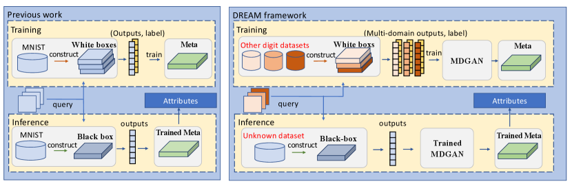
The work in [22] delves into model reverse engineering to reveal model attributes, as depicted in the left of Fig. 1. They first construct a large set of white-box models which are trained based on the same datasets as the target black-box model, , the MNIST hand-written dataset [23]. Then, the outputs of white-box models are obtained through a sequence of input queries. Finally, a meta-model is trained to learn a mapping between model outputs and model attributes. For inference, outputs of the target black-box model are fed into the meta-model to predict model attributes. The promising results demonstrate the feasibility of model reverse engineering.
However, a crucial limitation in [22] is that they assume the dataset used for training the target model to be known in advance, and leverage this dataset for meta-model learning.
In most application cases, the training data of a target black-box model is unknown. When the distribution of training data of the target black-box model is inconsistent with that of the set of constructed white-box models, the meta-model is usually unable to generalize well on the target black-box model.
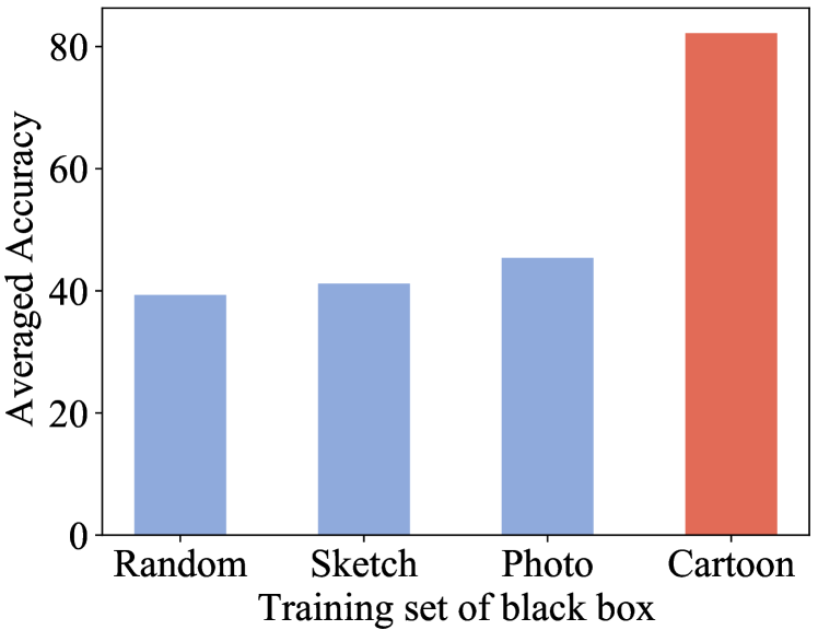
To verify this point, we train three black-box models with the same architecture on three different datasets, Photo, Cartoon and Sketch[24], respectively. Subsequently, we employ the approach outlined in [22] to train a meta-model using the white-box models trained specifically on the Cartoon dataset Then, we utilize the trained meta-model to infer attributes of the three black-box models.
The results are shown in Fig. 2. The y-axis represents the average accuracy of reverse engineering for each model attribute (e.g., activation function, optimizer, etc.). When the training dataset of black-box models and white-box models are the same (i.e., Cartoon), the performance reaches about . Otherwise, it sharply drops to about — close to random guess. This substantial gap underscores the non-trivial nature of investigate model reverse engineering, when the training dataset for the target black-box model is unavailable.
In this paper, we investigate the problem of reverse engineering the attributes of black-box models without requiring access to the target model’s training data. When the same input queries are fed to models with the same architecture but trained on different datasets, the output distributions typically differ. Therefore, a key point to our problem setting is bridging the gap between the output distributions of white-box and target black-box models, given the absence of the target model’s training data. An ideal meta-classifier should be well trained based on the outputs of white-box models, and predict well on outputs of the target black-box model, even if white-box and black-box models are trained on different types of data.
In light of this, we cast such a problem as an OOD generalization problem, and propose a novel framework DREAM: Domain-agnostic Reverse Engineering the Attributes of black-box Model, as shown in the right of Fig. 1. OOD generalization learning has been widely studied in recent years in the field of computer vision, and shows powerful performance [25, 26, 27]. Its goal is to learn a model on data from one or multiple domains and to generalize well on data from another domain that has not been seen during training. One kind of mainstream OOD learning approach is to extract domain-invariant features from data of multiple different domains, and utilize the domain-invariant features for downstream tasks [28, 29, 30, 31]. Returning to our problem, black-box models deployed on cloud platforms usually provide the label categories of their outputs. Therefore, we can collect data of different styles according to the model’s label space as OOD dataset. This overlap ensures that the outputs of the white-box models include similar information with those of the black-box model to some extent. Numerous white-box models are then trained on this OOD dataset, and we obtain outputs by querying these models. These outputs are used as source domains to achieve OOD generalization for reverse engineering black-box models.
Since the data we concentrate on is related to the outputs of models, , probability values, how to design an effective OOD generalization method over this type of data has not been explored. To this end, we introduce a multi-discriminator generative adversarial network (MDGAN) to learn domain-invariant features from the outputs of white-box models trained on multi-domain outputs. Based on these learned domain-invariant features, we learn a domain-agnostic reverse meta-model111The meta-model is used to infer the attributes of a model, thereby ”reverse-engineering” a black-box model into a white-box model. Hence, we name it the ”reverse meta-model”., which is capable of accurately inferring the attributes of the target black-box model trained on unknown data.
Our contributions are summarized as follows: 1) We provide the first study on the problem of domain-agnostic reverse engineering the attributes of black-box models and cast it as an OOD generalization problem; 2) We propose a generalized framework, DREAM, to address the problem of inferring the attributes of a black-box model with an unknown training dataset; 3) We constitute the first attempt to explore learning domain-invariant features from probability outputs, as opposed to traditional image; 4) We conduct extensive experiments to demonstrate the effectiveness of our method.
II Related Works
Reverse Engineering of Model Attributes. Its goal is to reveal attribute values of a target model, such as model structure, optimization method, hyperparameters, . Current research efforts focus on two aspects, hardware [32, 33, 34] and software [22, 35, 36, 37]. The hardware-based methods utilize information leaks from side-channel [33, 32] or unencrypted PCIe buses [34] to invert the structure of deep neural networks. Software-based methods reveal model attributes by machine learning. [35] steals the trade-off weight of the loss function and the regularization term. They derive over-determined linear equations and solve the hyperparameters by the least-square method. [37] theoretically proves the weight and bias can be reversed in linear network with ReLU activation. [38] infers hyperparamters and loss functions of generative models through the generated images. KENNEN [22] prepares a set of white-box models and then trains a meta-model to build a mapping between model outputs and their attributes. It is the most related work to ours. However, a significant difference is that KENNEN [22] requires the data used to train the target black-box model to be given beforehand. Our method relaxes this condition, , we no longer require the training data of the target model to be available, which is a more practical problem.
Model Functionality Extraction. It aims to train a clone model that has similar model functionality to that of the target model. To achieve this goal, many works have been proposed in recent years [39, 40, 41, 42, 16, 18, 19]. [39] uses an alternative dataset collected from the Internet to query the target model. [40] assumes part of the dataset is known and then presents a dataset augmentation method to construct the dataset for querying the target model. Moreover, data-free extraction methods [41, 40, 42, 43] query a target model through data generated by a generator, without any knowledge about the training data distribution. Different from the methods mentioned above, our goal is to infer the attributes of a black-box model, rather than stealing the model function.
Membership Inference. Its goal is to determine whether a sample belongs to the training set of a model [44, 45, 46, 47, 48, 49, 50, 51]. Although inferring model attribute is different from the task of membership inference, the technique in [22] is similar to those of membership inference attack. However, as stated aforementioned, when the domain of training data of the target black-box model is inconsistent with that of the set of white-box models, the method is usually unable to generalize well because of the OOD problem.
Out-of-distribution Generalization. Machine learning models often suffer from performance degradation during testing when the distribution of the training data (i.e., the source domains) differs from the test data distribution (i.e., the target domain). This is an out-of-distribution (OOD) problem. [25]. One straightforward approach is to leverage data from target domain to adapt the model trained on the source domains. This method is known as OOD adaptation, which has been successfully applied in image and video related tasks [52, 53, 54, 55]. However, in many application scenarios, data from the target domain is difficult to obtain. Therefore, OOD generalization methods are introduced [56, 57, 58, 59, 60], aiming to train a model by utilizing data from several source domains so that it can generalize well to any unseen OOD target domain. Existing OOD generalization methods mainly fall into three categories: invariant learning [29, 28, 30, 61, 62], causal learning [63, 64, 65, 66], and stable learning [67, 68, 69, 70]. Invariant learning seeks to minimize the differences among source domains to learn domain-invariant representations. Causal and stable learning aim to identify causal features linked to ground-truth labels from the data and filter out features unrelated to the labels. The former ensures the invariance of existing causal features, while the latter emphasizes effective features strongly related to labels by reweighting attention. Since the above methods primarily focus on images or videos, the design of an effective OOD learning method for attribute inference of black-box models has not been explored so far.
III Proposed Methods
In this section, we first introduce techinical background, threat model and problem formulation in Sect. III-A. Next, we describe the overall framework of our proposed DREAM in Sect. III-B. Subsequently, we delve into each components of DREAM in Sect. III-C to III-E. Finally, we introduce the training procedure in Sect. III-F.
III-A Preliminaries
We first introduce the background of the KENNEN method. Based on KENNEN, we present the threat model of the problem addressed in this paper. Finally, we introduce the problem formulation.
Background of KENNEN [22]. Given a black-box model , model attribute reverse engineering in [22] aims to build a meta-model , where is the outputs by querying the black-box model with queries , and is the set of model attributes including model architecture, optimizer, and training hyperparameters, . Concretely, they first construct a large set of white-box models containing different attributes combinations and train these white-box models based on the same training data as that of the target black-box model. Then outputs are obtained by querying these white-box models with a sequence of input image queries . Finally, they train a meta-model to build mappings from outputs to model attributes , where the subscript represents the type of attributes (, Activation, Dropout), while the superscript represents the value of the attributes (, ReLU/Tanh for Activation, Yes/No for Dropout). At the inference phase, the meta-model takes outputs from the target model as input and predicts the corresponding attributes.
Threat Model. Following KENNEN, we assume that attackers are permitted to query the model and can only access the probability outputs of the model, while attributes such as model structures and optimizers are unable to access. However, KENNEN makes a strong assumption that the training dataset of the model is known. In most cases, obtaining the training dataset is typically challenging. Therefore, we relax this assumption and consider a scenario where only the label space of the black-box model are known. This is a reasonable assumption because a black-box model deployed on the cloud platform typically provides information about its functionality and the categories it can output. Consequently, we can collect data with overlapping label spaces with the black-box target model. This overlap ensures that the outputs of the white-box models include similar information with those of the black-box model to some extent, thereby assisting in learning informative invariant features for achieving attributes reverse engineering.
Problem Formulation. As aforementioned, there is a strict constraint in [22] that they assume the training dataset of the target model to be given in advance, and leverage model outputs , where the models are trained on for the learning of meta-model . It is difficult to access the training data of a target black-box model, which significantly limits the applications of [22]. To mitigate this problem, we provide a new problem setting by relaxing the above constraint, , we no longer require the training data of the target black-box model to be available, but only the label space of the black-box model. Consequently, we cast this problem as an OOD generalization problem. To address this, we first collect data from different sources to train the white-box models. Although these data may contain different styles, all of them include an overlapping label space with the target black-box model. Then, the outputs obtained from the white-box models are divided into source domains according to the source of the training data for each model. In addition, the outputs from black-box model are the target domain. Our goal is to leverage outputs from source domains to train a domain-agnostic meta model that can well generalize to the outputs target domain, thereby enabling it to predict attributes for the target black-box model .
III-B DREAM Framework
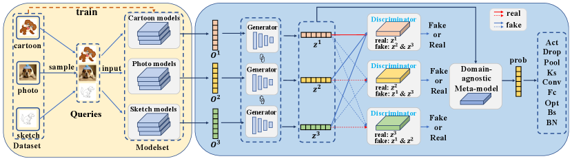
To perform domain-agnostic black-box model attribute reverse engineering, we cast this problem into an OOD generalization learning problem, and propose a novel framework DREAM, as shown in Fig. 3. Our DREAM framework consists of two parts:
In the left part of Fig. 3, we employ datasets from different domains to train numerous white-box models with diverse attributes, thereby constructing modelsets. (please refer to Sect. IV-A for more details). Next, we sample queries as input to these models. For each domain, we sample an equal number of images from the corresponding dataset and concatenate them as a batch of queries. These queries are sent to models belonging to the modelsets. The resulting multi-domain outputs are fed into the subsequent module of our DREAM framework. To learn domain-invariant features, we introduce a MDGAN, as shown in the right part of Fig. 3. MDGAN consists of multiple discriminators corresponding to different domains and one generator across multiple domains. The generator is designed to embed model outputs from different domains as features, while each discriminator strives to align the learned feature distributions from other domains with the feature distribution of the domain it corresponds to. In this way, the generator is capable of learning domain-invariant features. Based on the learned domain-invariant features, we further learn a domain-agnostic meta-model to infer the attributes of a black-box model with an unknown domain.
III-C Multi-domain Outputs Obtaining
To achieve model reverse engineering, we first need to obtain the multi-domain outputs of the white-box models. These outputs serve as features of white-box models’ attributes and will be used as inputs for the subsequent modules. We sample an equal number of images from the source dataset, resulting in queries , where is the number of total queries. Subsequently, these queries are fed into the white-box models , where represents models from the domain. For each domain , the models produces outputs , where is the number of classes in the dataset. We then concatenate the outputs as an 1-dimensional vector . Finally, the multi-domain outputs are derived as .
III-D Multi-Discriminator GAN
After preparing multi-domain outputs, we introduce MDGAN on the basis of [71]. The objective is to learn domain-invariant features from these probability outputs of white-box models trained on different domains.
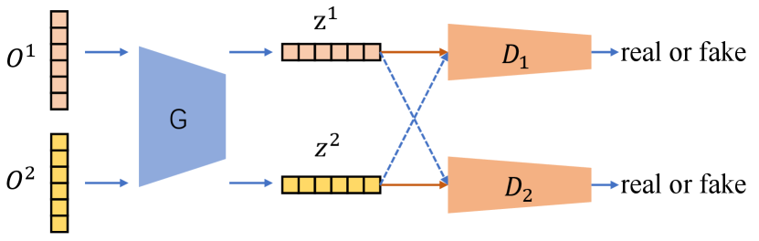
To better present, we take an example about how MDGAN works on two domains. As shown in Fig. 4, we have two kinds of inputs, and , from two domains. When feeding them into the generator , we can obtain the corresponding features and , respectively. After that, we feed and to the discriminator , where is expected to output a “real" label for and output a “fake" label for . By jointly training and based on a min-max optimization, the distribution of is expected to move towards that of . In the meantime, we also feed and to the discriminator . Differently, is expected to output a “real" label for and output a “fake" label for . By jointly training and , the distribution of is expected to move towards that of . In this way, and generated by the generator become domain-invariant representations.
Formally, we define . The generator sharing with parameter across domains maps outputs from the domain into the latent feature . After that, we obtain latent features of model outputs. We also define discriminators . Each discriminator outputs a scalar representing the probability that comes from the domain. The label of latent features is defined as Real for the discriminator when , while False when .
The training goal of is to maximize the log probability of assigning the correct label to features both from the domain and other domains, while the generator is trained against the discriminator to minimize the probability. In other words, it is a min-max game between the discriminator and generator with a value function , formulated as:
| (1) | ||||
During optimizing the min-max adversarial value function for and , the generator can gradually produce latent features from domain, which are close to latent features from other domain. Once and all are well trained, is able to embed multi-domain model outputs into an invariant feature space, where each discriminator cannot determine which domain the outputs are from. Therefore, the latent features become domain-invariant features. Note that our proposed MDGAN does not suffer from mode collapse. This is because mode collapse is an issue in generative tasks using GANs, where the model fails to generate diverse patterns and instead produces only a limited set of modes. In our approach, the role of generator in the MDGAN is not to generate diverse features. Instead, functions as an encoder, encoding the model’s outputs from different domains into invariant features. Therefore, it does not suffer from the problem of mode collapse.
III-E Domain-agnostic Reverse Meta-Model
After obtaining domain-invariant features , we aim to classify them as model attributes through the domain-agnostic reverse meta-model. Consider there are types of attributes and each attribute contains possible values, we build domain-agnostic reverse meta-models . Therefore, the probability for the attribute is obtained by:
| (2) |
Note that the is a -dimensional vector that contains attribute value, and each dimension represents the probability of the attribute value.
The target is to minimize the cross entropy between the predicted attributes probability and ground-truth of model attribute values :
| (3) |
During the inference phase, we input queries to the black-box model trained from an unknown domain to generate outputs. These outputs are then embedded as domain-invariant features by the generator . Subsequently, the reverse meta-model classifies these domain-invariant features, achieving domain-agnostic attributes predictions for the black-box model.
III-F Overall Objective and Training Strategy
After introducing all the components, we give the final loss function based on Eq. 1 and 3 as:
| (4) | ||||
where is a trade-off parameter.
The training strategy is as follows: we first optimize all discriminators , and then jointly optimize the generator and the domain-agnostic reverse meta-model. We repeat the above processes until the algorithm converges. The proposed optimization strategy is presented in Algorithm 1.
IV Experiments
| Attribute | Values |
| #Activation (act) | ReLU, PReLU, ELU, Tanh |
| #Dropout (drop) | Yes, No |
| #Max pooling (pool) | Yes, No |
| #Kernel size (ks) | 3, 5 |
| #Conv layers (conv) | 2, 3, 4 |
| #FC layers (fc) | 2, 3, 4 |
| #Optimizer (opt) | SGD, ADAM, RMSprop |
| #Batch size (bs) | 32, 64, 128 |
| #Batchnorm (bn) | Yes, No |
IV-A Dataset Construction
Following [22], we construct the modelset by training models that enumerate all possible attribute values. The details of the attributes and their values are shown in Table I. There are a total of types of attributes for each model in the modelsets, which adheres the following scheme: convolution layers, fully-connected layers 222Not that a model with more layers may be mistakenly classified as an overtrained model. However, this issue do not exist in practical applications, because we did not devise an attribute to determine if a model is overtrained. In practical applications, people tend to deploy models with strong generalization capabilities rather than overtrained ones. Therefore, to ensure accurate model reverse engineering, the white-box models we train are not overtrained either. We select the model that performs best on the validation set as the final white-box model, thereby ensuring its generalization performance.. Each convolution layer contains a kernel (), an optional batch normalization, an optional max-pooling, and a non-linear activation function in sequence. Each fully connected layer consists of a linear transformation, a non-linear activation, and an optional dropout in sequence. We set the dropout ratio to in our experiments. When training white-box models, optimizers are selected from SGD, ADAM, RMSprop with a batch size , or , respectively. The statistics of PACS modelset and MEDU modelset are listed in the Appendix.B By enumerating all possible model attributes, a total of distinct models can be obtained. In addition, we initialize each kind of model with random seeds from 0 and 999, yielding 5,184,000 unique models.
We construct PACS modelset and MEDU modelset to evaluate our method. The details are as follows:
PACS modelset comprises a set of models trained on the PACS dataset. The PACS dataset is an image dataset that has been widely used for OOD generalization [24]. We utilize 3 domains, including Photo (1,670 images), Cartoon (2,344 images), and Sketch (3,929 images), and each domain contains 7 kind of classes. For each modelset domain, we randomly sample and train 5,000, 1,000, and 1,000 from 5,184,000 white-box models as the training, validation, and testing models, respectively.
MEDU modelset consists of a set of models trained on MEDU dataset. MEDU is a hand-written digit recognition dataset, with 4 domains collected from MNIST [23], USPS [72], DIDA [73] and EMNIST [74]. Each domain contains different styles of hand-written digits from 0 to 9. Similar to PACS modelset, for each modelset domain, we randomly sample and train 5,000, 1,000, and 1,000 from 5,184,000 white-box models as the training, validation, and testing models.
IV-B Implementation Details of DREAM
In the experiment, we set the number of queries to 100. We use Adam [75] as the optimizer, where the learning rate is set to for the generator and discriminators, and the learning rate is set to for the domain-agnostic meta-model. The batch size is set as 100. The trade-off parameter is tuned from based on the validation set.
In addition, the MDGAN is composed of a generator and multiple discriminators. The generator consists of two linear layers with ReLU activation. The dimension of the input layer of the generator is determined by the query number and class category number . As for the experiment conducted on MEDU modelset, the input dimension is (the query number is , and the number of classes if ). In the case of the PACS modelset, the input dimension is 700 (, ). The output dimensions of the subsequent two linear layers are 500 and 128, respectively. Each discriminator consists of three linear layers. The first two layers employ ReLU as the activation function, while the last layer utilizes the Sigmoid activation function. The output dimensions of discriminator layers are 512, 256, and 1 respectively. Additionally, we implement the domain agnostic meta-models as MLPs. Each MLP consists of 3 layers, and it takes latent features produced by generator as input. The output dimensions of the MLP are 128, 64 and . All experiments are conducted on 4 NVIDIA RTX 3090 GPUs, PyTorch 1.11.0 platform [76].
IV-C Baselines
We compare our DREAM with 7 baselines including Random choice, SVM, KENNEN [22], SelfReg [29], MixStyle [30], MMD [28] and SD [77]. Additionally, we take four typical OOD generalization methods—SelfReg, MixStyle, MMD, and SD—as baselines to validate the effectiveness of our framework in learning domain-invariant features.
The details of the baseline methods are presented as follows:
SVM. The SVM serves as a baseline, representing a non-deep learning method. We directly input the multi-domain probability outputs into SVM classifiers to predict attributes. We adopt the One-vs-One (OvO) strategy. Specifically, for an attribute with possible values, we trained a binary SVM for each pair of attribute values, resulting in a total of SVMs. When classifying a new sample, we apply all trained SVM classifiers and use a voting mechanism for each attribute value. The attribute value receiving the most votes is selected as the final prediction. For 2-valued attributes, we only need to train a single binary SVM.
KENNEN*. We employ a variant of KENNEN (denoted as KENNEN* ). It takes fixed queries as input, which is the same as our approach. We embed the multi-domain probability outputs into feature space and use MLPs to predict attributes. Similar to SVM, KENNEN does not differentiate between outputs from different domains. In addition, to ensure a fair comparison, the network structure keeps consistent with the domain-agnostic reverse meta-model in DREAM.
SelfReg, MixStyle, MMD and SD. The approach taken by SelfReg to learn invariant features involves pulling samples of similar categories between all domains closer together while pushing samples of different categories further apart. The motivation behind MixStyle is based on the observation that the styles of domain images share significant similarities. In particular, MixStyle captures style information through the final layer and performs style mixing at that layer. The MMD adopts maximum mean discrepancy loss between each two domains. The SD proposes the Spectral Decoupling method to relieve the gradient starvation phenomenon during the training of the network, to boost the performance of OOD generalization. We embed the multi-domain probability outputs into feature space and apply the OOD generalization method, SelfReg, MixStyle, MMD, and SD, respectively to learn invariant features. Then the learned invariant features are fed into MLPs for predicting attributes. For a fair comparison, the network structure of MLPs is consistent with the domain-agnostic reverse meta-model in DREAM.
We adopt the leave-one-domain-out strategy to split the source and target domains for PACS and MEDU modelsets. For each modelset, we take one domain as the target domain and the rest as source domains in turn. The experiment is run for 10 trials, and the average results are reported.
| Target Domain | Method | Attributes | Avg | ||||||||
| #act | #drop | #pool | #ks | #conv | #fc | #opt | #bs | #bn | |||
| Random | 25.00 | 50.00 | 50.00 | 50.00 | 33.33 | 33.33 | 33.33 | 33.33 | 50.00 | 39.81 | |
| Photo | SVM | 37.80 | 50.30 | 54.80 | 53.60 | 34.00 | 36.60 | 37.00 | 45.70 | 58.80 | 45.40 |
| KENNEN* | 39.07 | 50.68 | 59.42 | 61.31 | 36.18 | 39.33 | 37.88 | 44.16 | 59.74 | 47.53 | |
| SelfReg | 25.58 | 52.26 | 54.98 | 50.18 | 34.12 | 35.25 | 34.61 | 33.78 | 50.76 | 41.28 | |
| MixStyle | 39.63 | 53.23 | 61.83 | 59.44 | 35.66 | 38.75 | 37.89 | 43.75 | 57.09 | 47.47 | |
| MMD | 38.88 | 54.70 | 60.46 | 56.54 | 35.38 | 36.66 | 35.66 | 40.50 | 61.04 | 46.65 | |
| SD | 38.70 | 51.06 | 58.86 | 62.21 | 35.84 | 40.05 | 39.23 | 44.34 | 62.12 | 48.04 | |
| DREAM | 43.84 | 59.19 | 66.09 | 64.24 | 39.59 | 42.04 | 40.49 | 47.83 | 68.12 | 52.38 | |
| Cartoon | SVM | 25.80 | 49.20 | 50.70 | 55.80 | 37.20 | 38.10 | 30.80 | 42.30 | 65.30 | 43.91 |
| KENNEN* | 32.99 | 52.50 | 54.23 | 56.57 | 37.19 | 40.53 | 33.47 | 37.17 | 68.39 | 45.89 | |
| SelfReg | 25.97 | 51.42 | 56.20 | 50.03 | 35.04 | 35.52 | 36.09 | 35.58 | 56.17 | 42.44 | |
| MixStyle | 32.10 | 50.76 | 55.44 | 54.18 | 36.18 | 37.87 | 34.65 | 38.69 | 60.26 | 44.46 | |
| MMD | 29.56 | 53.02 | 54.70 | 53.82 | 35.38 | 36.36 | 35.98 | 37.24 | 57.58 | 43.75 | |
| SD | 33.52 | 54.06 | 54.12 | 56.69 | 36.84 | 41.02 | 35.61 | 36.12 | 65.12 | 45.90 | |
| DREAM | 37.53 | 55.89 | 61.18 | 57.32 | 38.58 | 39.60 | 38.32 | 45.01 | 65.16 | 48.73 | |
| Sketch | SVM | 23.80 | 47.60 | 47.40 | 45.80 | 33.80 | 34.50 | 31.80 | 34.30 | 53.10 | 39.12 |
| KENNEN* | 34.64 | 50.10 | 53.07 | 52.01 | 34.61 | 37.11 | 35.78 | 37.04 | 55.27 | 43.29 | |
| SelfReg | 27.07 | 54.32 | 51.39 | 53.07 | 36.99 | 36.82 | 35.47 | 34.17 | 61.80 | 43.46 | |
| MixStyle | 37.78 | 51.71 | 54.16 | 53.60 | 34.53 | 36.16 | 36.36 | 36.02 | 59.42 | 44.42 | |
| MMD | 31.96 | 52.94 | 56.84 | 52.78 | 38.18 | 38.20 | 36.20 | 35.92 | 57.56 | 44.51 | |
| SD | 34.82 | 52.51 | 56.89 | 51.21 | 34.23 | 38.12 | 35.91 | 36.72 | 54.23 | 43.85 | |
| DREAM | 39.71 | 57.74 | 64.73 | 60.79 | 40.79 | 40.14 | 43.54 | 43.80 | 72.51 | 51.53 | |
| Target Domain | Method | Attributes | Avg | ||||||||
| #act | #drop | #pool | #ks | #conv | #fc | #opt | #bs | #bn | |||
| Random | 25.00 | 50.00 | 50.00 | 50.00 | 33.33 | 33.33 | 33.33 | 33.33 | 50.00 | 39.81 | |
| MNIST | SVM | 45.60 | 49.40 | 62.90 | 59.20 | 38.80 | 40.10 | 35.50 | 35.00 | 75.30 | 49.09 |
| KENNEN* | 51.18 | 50.67 | 62.99 | 57.36 | 38.32 | 35.84 | 41.57 | 35.75 | 77.87 | 50.17 | |
| SelfReg | 28.00 | 53.57 | 53.43 | 50.78 | 35.97 | 36.39 | 35.98 | 36.23 | 53.96 | 42.70 | |
| MixStyle | 50.27 | 51.72 | 62.66 | 57.32 | 37.88 | 36.34 | 43.11 | 38.00 | 82.61 | 51.10 | |
| MMD | 44.57 | 59.67 | 66.37 | 57.27 | 39.63 | 37.27 | 42.10 | 37.60 | 81.37 | 51.76 | |
| SD | 49.60 | 49.40 | 62.40 | 52.30 | 37.10 | 36.70 | 38.90 | 35.30 | 81.50 | 49.24 | |
| DREAM | 51.01 | 62.32 | 64.28 | 58.39 | 40.96 | 38.11 | 45.37 | 38.96 | 81.99 | 53.49 | |
| EMNIST | SVM | 40.00 | 48.70 | 69.20 | 51.60 | 40.20 | 36.90 | 35.80 | 30.10 | 79.90 | 48.04 |
| KENNEN* | 45.66 | 51.01 | 65.26 | 53.25 | 40.28 | 36.35 | 41.96 | 36.16 | 81.30 | 50.14 | |
| SelfReg | 27.29 | 52.83 | 53.32 | 52.85 | 33.68 | 35.05 | 35.26 | 35.32 | 53.74 | 42.15 | |
| MixStyle | 43.68 | 51.35 | 67.87 | 57.15 | 42.50 | 39.30 | 42.10 | 38.79 | 82.46 | 51.69 | |
| MMD | 42.03 | 58.43 | 66.27 | 60.80 | 40.80 | 38.67 | 40.00 | 39.97 | 84.00 | 52.33 | |
| SD | 43.60 | 48.90 | 59.20 | 60.10 | 44.50 | 35.10 | 43.60 | 33.80 | 88.80 | 50.84 | |
| DREAM | 45.55 | 64.98 | 74.16 | 60.71 | 44.45 | 42.45 | 47.37 | 41.03 | 91.00 | 56.86 | |
| DIDA | SVM | 45.00 | 47.80 | 54.60 | 45.50 | 29.40 | 37.60 | 43.30 | 36.50 | 63.70 | 44.82 |
| KENNEN* | 42.73 | 52.06 | 55.27 | 52.02 | 34.89 | 38.90 | 38.98 | 36.27 | 54.97 | 45.12 | |
| SelfReg | 26.31 | 54.29 | 53.23 | 52.33 | 34.96 | 35.72 | 36.49 | 35.39 | 59.11 | 43.09 | |
| MixStyle | 45.26 | 52.32 | 55.91 | 51.39 | 34.22 | 38.70 | 38.31 | 38.03 | 57.44 | 45.73 | |
| MMD | 39.00 | 59.20 | 59.63 | 55.93 | 35.93 | 38.33 | 37.93 | 37.50 | 54.40 | 46.43 | |
| SD | 46.50 | 51.80 | 52.70 | 51.90 | 34.90 | 45.30 | 42.70 | 36.80 | 59.50 | 46.92 | |
| DREAM | 49.63 | 64.50 | 59.30 | 57.13 | 39.52 | 44.59 | 42.09 | 40.19 | 59.68 | 50.74 | |
| USPS | SVM | 43.40 | 50.50 | 47.60 | 52.50 | 30.30 | 32.30 | 41.00 | 36.60 | 49.40 | 42.62 |
| KENNEN* | 43.38 | 50.88 | 51.41 | 53.19 | 36.35 | 35.59 | 36.66 | 34.56 | 55.62 | 44.18 | |
| SelfReg | 26.81 | 52.16 | 55.46 | 52.47 | 36.18 | 36.43 | 36.53 | 35.90 | 55.34 | 43.03 | |
| MixStyle | 41.05 | 53.80 | 50.49 | 52.93 | 35.26 | 33.68 | 36.92 | 34.75 | 59.34 | 44.25 | |
| MMD | 39.33 | 55.87 | 52.67 | 53.23 | 39.20 | 34.33 | 35.90 | 36.90 | 60.73 | 45.35 | |
| SD | 41.90 | 50.40 | 58.00 | 52.30 | 33.10 | 35.30 | 36.60 | 34.30 | 61.60 | 44.83 | |
| DREAM | 42.34 | 58.72 | 58.58 | 54.41 | 37.90 | 37.81 | 40.42 | 38.36 | 63.39 | 47.99 | |
| Dataset | Victim Model | Architecture of the Extraction Model | ||
| #Same to Victim | #Random | #Inferred by DREAM | ||
| MNIST | ||||
| Target Domain | Method | Attributes | Avg | ||||||||
| #act | #drop | #pool | #ks | #conv | #fc | #opt | #bs | #bn | |||
| Random | 25.00 | 50.00 | 50.00 | 50.00 | 33.33 | 33.33 | 33.33 | 33.33 | 50.00 | 39.81 | |
| Sketch | SVM | 23.80 | 47.60 | 47.40 | 45.80 | 33.80 | 34.50 | 31.80 | 34.30 | 53.10 | 39.12 |
| KENNEN* | 34.64 | 50.10 | 53.07 | 52.01 | 34.61 | 37.11 | 35.78 | 37.04 | 55.27 | 43.29 | |
| SelfReg | 27.07 | 54.32 | 51.39 | 53.07 | 36.99 | 36.82 | 35.47 | 34.17 | 61.80 | 43.46 | |
| MixStyle | 37.78 | 51.71 | 54.16 | 53.60 | 34.53 | 36.16 | 36.36 | 36.02 | 59.42 | 44.42 | |
| MMD | 31.96 | 52.94 | 56.84 | 52.78 | 38.18 | 38.20 | 36.20 | 35.92 | 57.56 | 44.51 | |
| SD | 34.82 | 52.51 | 56.89 | 51.21 | 34.23 | 38.12 | 35.91 | 36.72 | 54.23 | 43.85 | |
| DREAM | 39.71 | 57.74 | 64.73 | 60.79 | 40.79 | 40.14 | 43.54 | 43.80 | 72.51 | 51.53 | |
| DREAM* | 42.24 | 55.68 | 61.82 | 58.34 | 39.55 | 38.39 | 38.51 | 41.39 | 74.39 | 50.03 | |
| Target Domain | Method | Attributes | Avg | ||||||||
| #act | #drop | #pool | #ks | #conv | #fc | #opt | #bs | #bn | |||
| Random | 25.00 | 50.00 | 50.00 | 50.00 | 33.33 | 33.33 | 33.33 | 33.33 | 50.00 | 39.81 | |
| CIFAR | SVM | 33.91 | 49.85 | 51.87 | 50.45 | 36.43 | 36.23 | 33.80 | 41.78 | 58.73 | 43.67 |
| KENNEN* | 38.65 | 56.71 | 56.21 | 56.71 | 36.73 | 39.35 | 41.68 | 44.30 | 63.57 | 48.21 | |
| SelfReg | 39.46 | 52.17 | 60.44 | 55.60 | 38.65 | 40.46 | 47.12 | 47.53 | 61.45 | 49.21 | |
| MixStyle | 41.78 | 53.48 | 57.52 | 53.18 | 36.93 | 41.68 | 43.59 | 46.72 | 63.98 | 48.76 | |
| MMD | 40.46 | 60.54 | 59.54 | 57.32 | 37.94 | 43.49 | 48.84 | 50.25 | 67.00 | 51.71 | |
| SD | 39.05 | 53.78 | 57.92 | 56.51 | 36.23 | 41.78 | 41.47 | 50.76 | 67.31 | 49.42 | |
| DREAM | 45.11 | 62.36 | 61.35 | 61.76 | 41.88 | 45.41 | 47.53 | 49.85 | 75.88 | 54.57 | |
IV-D Comparison with Baselines
Table II and III report the overall performance of different methods on the PACS modelset and MEDU modelset, respectively. The leftmost column in each table indicates the target domain (the rest ones are source domains). In this experiment, we adopt the complete overlap setting, where the label space of the source domain and target domain is identical. The performance achieved by our proposed DREAM is better than that of all baselines in terms of the average accuracy of model attributes. For individual attribute, our method outperforms other methods in most cases. DREAM demonstrates superior performance compared to KENNEN and SVM. This suggests that, in situations where the training dataset of the target black-box model is unknown, utilizing our proposed MDGAN for learning invariant features, instead of directly inputting the outputs from the source domain into the meta-model for attribute prediction, results in enhanced generalization. DREAM also outperforms four OOD generalization methods, which highlights the superior capability of the proposed MDGAN in learning domain-invariant features from probability outputs compared to other baselines.
IV-E Application Value of Model Reverse Engineering
To show the application value of our method, we conduct a model extraction experiment. We adopt a popular model extraction method MAZE [41], where model structures are "Same to the victim", "Random", or "Inferred by DREAM". As shown in Table IV, The performance of model extraction using the architecture "Inferred by DREAM" significantly outperforms that achieved with a random architecture ( vs. ). Moreover, its performance closely approaches that obtained when employing the "Same as the victim" architecture for model extraction ( vs. ). The rationale behind above results lies in the fact that extraction performance improves when the structure of the extracted model closely aligns with that of the victim, as discussed in [21]. The proximity of the extracted model to the victim model in terms of structure and complexity enhances the likelihood of capturing identical patterns and information present in the victim model.
IV-F Visualization of Generated Feature Space
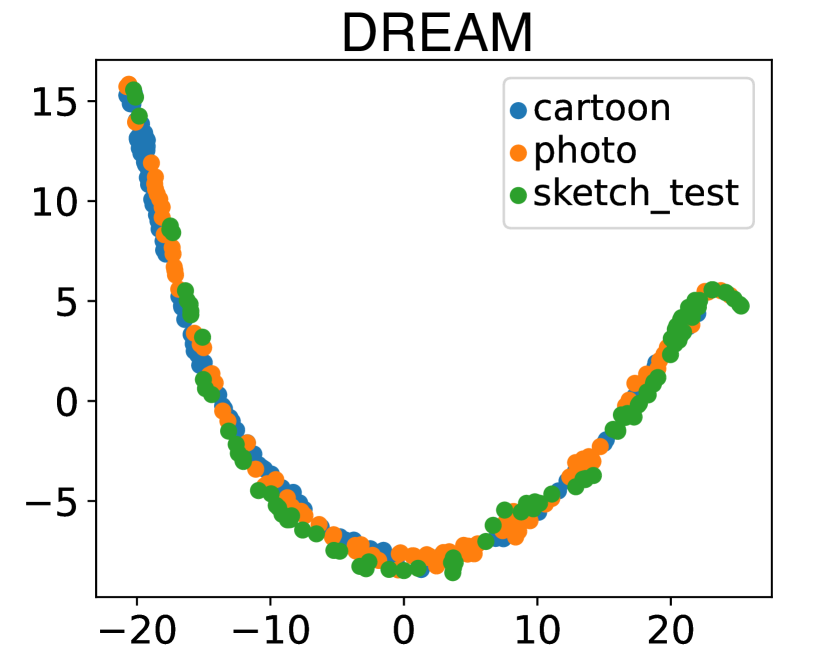
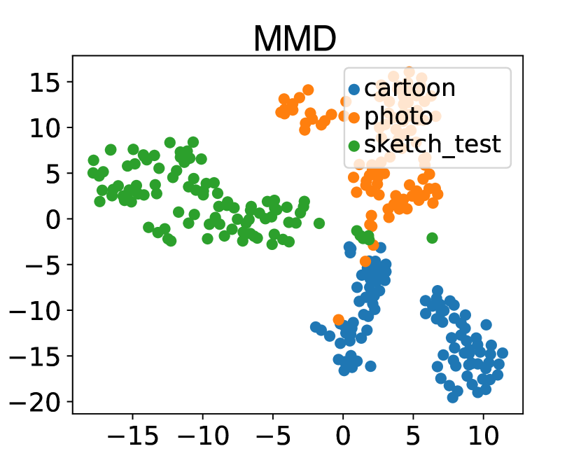
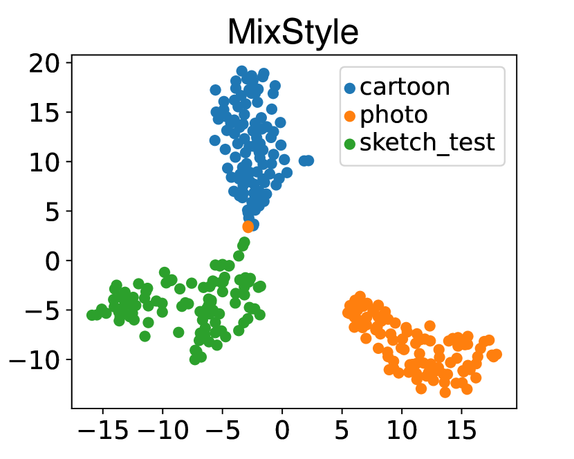
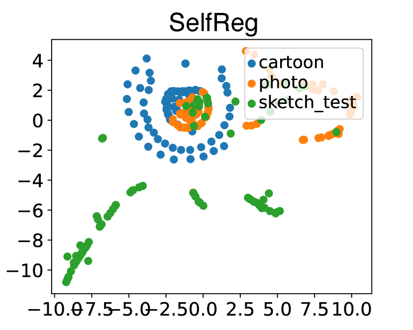
To further verify the effectiveness of our method, we utilize t-SNE [78] to visualize samples in the feature space learned by the generator of our framework. The visualization is carried out on PACS modelset. We take C (cartoon) and P (photo) as source domains to train white-box models, and use S (sketch) as the unseen target domain to the train black-box model. In this experiment, we adopt the complete overlap setting. As shown in Fig. 5, we observe the features from sources and target domain are spread in the feature space for MMD, MixStyle and SelfReg method. However, DREAM can embed samples from both the source domains and target domain into an invariant feature space, which demonstrates the superiority of DREAM.
IV-G Experiment on Domain Shift Scenario
1) We conduct class shift experiment on PACS modelset. In this experiment, we exclude the "dog" and "elephant" classes among 7 classes for each source domain while constructing white-box models, while the target domain remain all 7 classes. As shown in Table V, the average accuracy of DREAM* reaches 50.03%. Although DREAM* experiences a slight decrease in accuracy compared to DREAM due to domain shift, it still outperforms other baselines.
| Target Domain | Method | Attributes | Avg | ||||||||
| #act | #drop | #pool | #ks | #conv | #fc | #opt | #bs | #bn | |||
| Random | 25.00 | 50.00 | 50.00 | 50.00 | 33.33 | 33.33 | 33.33 | 33.33 | 50.00 | 39.81 | |
| Photo | SVM | 34.20 | 51.70 | 48.50 | 56.10 | 35.70 | 36.50 | 37.60 | 40.50 | 64.60 | 45.04 |
| KENNEN* | 37.36 | 53.12 | 57.79 | 59.66 | 38.94 | 35.93 | 37.92 | 41.71 | 63.91 | 47.37 | |
| SelfReg | 26.08 | 52.35 | 53.89 | 52.70 | 35.11 | 33.84 | 37.46 | 36.42 | 50.99 | 42.09 | |
| MixStyle | 35.98 | 54.31 | 57.35 | 57.43 | 37.14 | 35.51 | 39.31 | 42.07 | 57.84 | 46.33 | |
| MMD | 38.67 | 57.16 | 61.49 | 58.73 | 40.65 | 39.14 | 38.69 | 41.06 | 71.48 | 49.67 | |
| SD | 38.70 | 51.06 | 58.86 | 62.21 | 35.84 | 40.05 | 39.23 | 44.34 | 62.12 | 48.04 | |
| DREAM | 43.84 | 59.19 | 66.09 | 64.24 | 39.59 | 42.04 | 40.49 | 47.83 | 68.12 | 52.38 | |
| DREAM** | 39.68 | 57.61 | 64.48 | 60.79 | 40.78 | 40.10 | 43.54 | 43.80 | 72.42 | 51.47 | |
2) We conduct experiments in situations where domains are quite different, and number of classes between domains are different. We first train white-box models using the Sketch and Cartoon datasets. The outputs of these white-box models serve as the source domains for training DREAM. We then utilized data from CIFAR10 and CIFAR100 to train black-box models. The trained DREAM infers attributes based on the black-box model outputs. The source domains (Sketch and Cartoon) comprise 7 classes, while the target domain (CIFAR10/100) contains 110 classes. We use all 7 classes as the label space for the source domains. For the target domain’s label space, we select the 5 classes that overlap between the source and target domains (namely: dog, elephant, house, horse, and person). This ensures a overlapping label space, but different number of classes between source and target domains. The experimental results are listed in Table VI, which demonstrate that DREAM still outperforms Random, KENNEN, as well as state-of-the-art OOD generalization approaches. This indicates that our method is effective when domains are quite different, as well as when the number of classes differs between domains.


3) We investigate the shift scenario where white-box models used for training meta-model and the black-box model to be inferred have completely different attribute combinations. As mentioned in Sect. IV-A, there are a total of combinations of model attributes. We randomly select , , and models for the training, validation, and testing sets, respectively, ensuring that none of the models share identical attribute combinations. We adopt the complete overlap setting. The resulting model is denoted as DREAM**. As demonstrated in Table VII, DREAM** consistently outperforms other baselines under this setting. Consequently, the shift caused by attribute combinations does not significantly impact its overall performance.
IV-H Analysis
We analyse the size of modelset and the training data amount. We adopt the complete overlap setting in these two experiments.
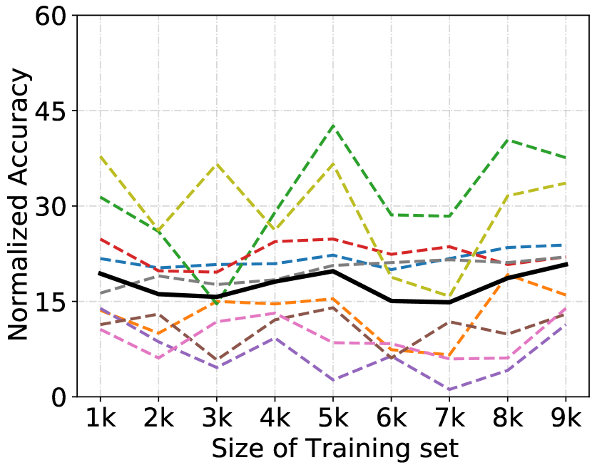
Analysis of Size of Modelset. We further study the performance of our method against the size of the PACS modelset. As shown in Fig. 6, we observe that the performance slightly fluctuates from the size of 1K to 5K, and does not consistently increase when the size increases. We suspect it can be attributed to the difficulty of our problem for domain-agnostic attribute inference of the black-box model, and the nature of the OOD problem, , the noise level increases as the size of the model set increases. It is worth studying further.
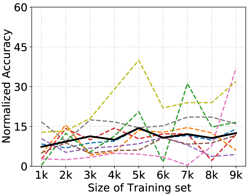
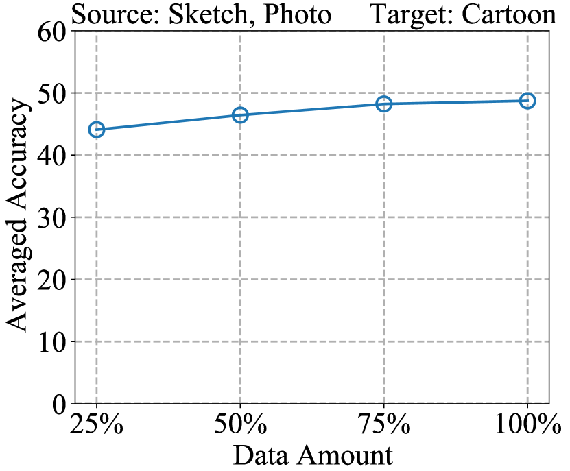
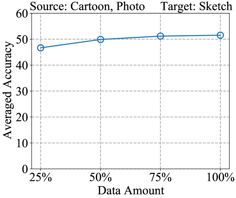
Analysis of Training Data Amount. We analyze the impact of amount of training samples on reverse engineering performance. We train white-box models using 25%, 50%, 75%, and 100% of PACS training data, respectively. We then apply our proposed DREAM method to perform reverse engineering on these models. The results are presented in Fig. 7. We observe as the amount of data increases, the performance improves, and the performance levels off when the amount of data reaches 75%.
IV-I Reverse Engineering on Model with Larger Attribute Space
We design a larger model attribute space for model attribute inference, as shown in Table IX. Specifically, we
-
•
Add "GeLU" activation function to the "#Activation" attribute space.
-
•
Expand "#Kernel size" attribute space from to
-
•
Expand "#Conv layers" attribute space from to
-
•
increase "#FC layers" attribute space from to .
The outputs of models trained on the Photo and Cartoon datasets serve as the source domains in this experiment, whereas those trained on the Sketch dataset function as the target domain. We adopt the complete overlap setting in this experiment. The results presented in Table X demonstrate that our method continues to outperform the baseline methods.
| Attribute | Values |
| #Activation (act) | ReLU, PReLU, ELU, Tanh, GeLU |
| #Dropout (drop) | Yes, No |
| #Max pooling (pool) | Yes, No |
| #Kernel size (ks) | 3, 4, 5, 6, 7, 8, 9 |
| #Conv layers (conv) | 2, 3, 4, 5, 6, 7, 8, 9, 10, 11 |
| #FC layers (fc) | 2, 3, 4, 5, 6, 7, 8 |
| #Optimizer (opt) | SGD, ADAM, RMSprop |
| #Batch size (bs) | 32, 64, 128 |
| #Batchnorm (bn) | Yes, No |
| Attribute | Values |
| #Activation (act) | ReLU, PReLU, ELU, Tanh, GeLU |
| #Dropout (drop) | Yes, No |
| #Patch size (ps) | 2, 4, 8, 16 |
| #Transformer layers (n_trans) | 2, 3, 4, 5, 6, 7, 8, 9,10 |
| #Feedforward layers (n_ff) | 2, 3, 4 |
| #Attention heads (n_heads) | 1, 2, 4, 6, 8, 12 |
| #Optimizer (opt) | SGD, ADAM, RMSprop |
| #Batch size (bs) | 16, 32, 64 |
| Target Domain | Method | Attributes | Avg | ||||||||
| #act | #drop | #pool | #ks | #conv | #fc | #opt | #bs | #bn | |||
| Random | 20.00 | 50.00 | 50.00 | 14.29 | 10.00 | 14.29 | 33.33 | 33.33 | 50.00 | 30.58 | |
| Sketch | SVM | 36.32 | 58.74 | 60.91 | 17.39 | 10.80 | 17.18 | 54.53 | 35.70 | 69.24 | 40.09 |
| KENNEN* | 35.29 | 64.61 | 68.31 | 19.75 | 15.33 | 20.99 | 62.45 | 39.40 | 69.34 | 43.94 | |
| SelfReg | 37.86 | 62.65 | 66.98 | 20.37 | 16.46 | 21.91 | 66.87 | 39.09 | 66.56 | 44.31 | |
| MixStyle | 35.91 | 60.80 | 66.77 | 19.14 | 17.49 | 19.75 | 64.81 | 40.43 | 67.59 | 43.63 | |
| MMD | 36.52 | 64.61 | 68.72 | 19.96 | 15.64 | 19.24 | 68.93 | 38.89 | 70.37 | 44.76 | |
| SD | 35.08 | 65.43 | 65.33 | 20.06 | 15.95 | 21.50 | 63.99 | 39.40 | 67.39 | 43.79 | |
| DREAM | 40.53 | 66.77 | 68.93 | 25.51 | 20.68 | 24.79 | 69.34 | 44.75 | 72.94 | 48.25 | |
| Target Domain | Method | Attributes | Avg | |||||||
| #act | #drop | #ps | #n_trans | #n_ffn | #n_head | #opt | #bs | |||
| Random | 20.00 | 50.00 | 25.00 | 11.11 | 33.33 | 16.67 | 33.33 | 33.33 | 27.85 | |
| Sketch | SVM | 25.31 | 52.47 | 45.27 | 14.20 | 37.45 | 25.31 | 46.30 | 41.98 | 36.03 |
| KENNEN* | 28.40 | 64.20 | 53.29 | 16.26 | 43.83 | 25.51 | 51.03 | 54.32 | 42.10 | |
| SelfReg | 28.19 | 65.64 | 40.74 | 17.08 | 51.65 | 29.84 | 42.39 | 59.47 | 41.87 | |
| MixStyle | 25.51 | 59.88 | 46.91 | 15.43 | 45.47 | 26.75 | 45.47 | 54.73 | 40.02 | |
| MMD | 27.57 | 56.38 | 53.29 | 18.93 | 48.56 | 29.84 | 39.09 | 56.58 | 41.44 | |
| SD | 29.84 | 59.47 | 56.38 | 17.28 | 45.06 | 28.19 | 43.83 | 53.29 | 41.67 | |
| DREAM | 34.36 | 68.93 | 54.73 | 20.37 | 49.79 | 31.28 | 57.00 | 61.11 | 47.20 | |
IV-J Reverse Engineering on Vision Transformer Architecture
In addition to performing attribute inference on CNN architecture, we extend our approach to Vision Transformer (ViT) architecture. The Vision Transformer (ViT) applies the Transformer architecture, originally used in natural language processing, to images. Specifically, it divides an image into several patches and uses a Transformer to extract features from the image [79]. We design an attribute space for the Vision Transformer architecture, as shown in Table IX. #Patch size = means that each input image is divided into patches of size , which are used as the input to the ViT. Additionally, we include the number of #Transformer layers, #Feedforward layers, and numbers of #Attention heads in the attribute space. In this experiment, we also use outputs from models trained on the Photo and Cartoon datasets as the source domains, and outputs from models trained on the Sketch dataset as the target domain. The complete overlap setting is adopted. The experimental results, listed in Table XI, indicate that our method is capable of effectively performing attribute inference for Vision Transformer models, outperforming other baseline methods.
V Limitations and Future Works
DREAM requires training white-box models with numerous attribute combinations to ensure the performance of reverse engineering, which costs significant computational resources. For instance, when constructing the PACS modelset, each model requires approximately 5 minutes of training time. Consequently, the total training time for 13,000 models (10,000 for training, 2,000 for validation, and 1,000 for testing) amounts to roughly 45 GPU-days. To reduce these costs, one plausible approach is to leverage fewer white-box models for reverse engineering. Considering the relationships among attributes, we can design a multi-task learning method, where reverse engineering each attribute is treated as a task, to maintain the performance in the future.
VI Conclusion
In this paper, we studied the problem of domain-agnostic reverse engineering towards the attributes of the black-box model with unknown traning dataset, and cast it as an OOD generalization problem. We proposed a generalized framework, DREAM, which can predict the attributes of a black-box model with an unknown domain, and explored to learn domain-invariant features from probability outputs in the scenario of black-box attribute inference. Extensive experimental results demonstrated the effectiveness of our method.
ACKNOWLEDGEMENT
This work was supported by the NSFC under Grants 62122013, U2001211. This work was also supported by the Innovative Development Joint Fund Key Projects of Shandong NSF under Grants ZR2022LZH007.
References
- [1] A. Iscen, A. Fathi, and C. Schmid, “Improving image recognition by retrieving from web-scale image-text data,” in Proceedings of the IEEE/CVF Conference on Computer Vision and Pattern Recognition, 2023, pp. 19 295–19 304.
- [2] X. Ding, Y. Zhang, Y. Ge, S. Zhao, L. Song, X. Yue, and Y. Shan, “Unireplknet: A universal perception large-kernel convnet for audio video point cloud time-series and image recognition,” in Proceedings of the IEEE/CVF Conference on Computer Vision and Pattern Recognition, 2024, pp. 5513–5524.
- [3] X. Zhou and O. Wu, “Implicit counterfactual data augmentation for deep neural networks,” arXiv preprint arXiv:2304.13431, 2023.
- [4] C. Li, R. Li, Y. Yuan, G. Wang, and D. Xu, “Deep unsupervised active learning via matrix sketching,” IEEE Transactions on Image Processing, vol. 30, pp. 9280–9293, 2021.
- [5] Y.-C. Lin, S.-A. Chen, J.-J. Liu, and C.-J. Lin, “Linear classifier: An often-forgotten baseline for text classification,” in Proceedings of the 61st Annual Meeting of the Association for Computational Linguistics (Volume 2: Short Papers), A. Rogers, J. Boyd-Graber, and N. Okazaki, Eds. Toronto, Canada: Association for Computational Linguistics, Jul. 2023, pp. 1876–1888. [Online]. Available: https://aclanthology.org/2023.acl-short.160
- [6] E. Tanwar, S. Dutta, M. Borthakur, and T. Chakraborty, “Multilingual llms are better cross-lingual in-context learners with alignment,” in Proceedings of the 61st Annual Meeting of the Association for Computational Linguistics (Volume 1: Long Papers), 2023, pp. 6292–6307.
- [7] Y. Zhu, Y. Ye, M. Li, J. Zhang, and O. Wu, “Investigating annotation noise for named entity recognition,” Neural Computing and Applications, vol. 35, no. 1, pp. 993–1007, 2023.
- [8] L. Yang, H. Chen, Z. Li, X. Ding, and X. Wu, “Give us the facts: Enhancing large language models with knowledge graphs for fact-aware language modeling,” IEEE Transactions on Knowledge and Data Engineering, 2024.
- [9] M. Mulimani and A. Mesaros, “Class-incremental learning for multi-label audio classification,” in ICASSP 2024 - 2024 IEEE International Conference on Acoustics, Speech and Signal Processing (ICASSP), 2024, pp. 916–920.
- [10] A. Axyonov, D. Ryumin, D. Ivanko, A. Kashevnik, and A. Karpov, “Audio-visual speech recognition in-the-wild: Multi-angle vehicle cabin corpus and attention-based method,” in ICASSP 2024 - 2024 IEEE International Conference on Acoustics, Speech and Signal Processing (ICASSP), 2024, pp. 8195–8199.
- [11] X.-C. Li, X.-Y. Zhang, F. Yin, and C.-L. Liu, “Decision-based adversarial attack with frequency mixup,” IEEE Transactions on Information Forensics and Security, vol. 17, pp. 1038–1052, 2022.
- [12] J. Li, T. Xie, L. Chen, F. Xie, X. He, and Z. Zheng, “Adversarial attack on large scale graph,” IEEE Transactions on Knowledge and Data Engineering, vol. 35, no. 1, pp. 82–95, 2021.
- [13] H. Chang, Y. Rong, T. Xu, W. Huang, H. Zhang, P. Cui, X. Wang, W. Zhu, and J. Huang, “Adversarial attack framework on graph embedding models with limited knowledge,” IEEE Transactions on Knowledge and Data Engineering, vol. 35, no. 5, pp. 4499–4513, 2022.
- [14] H. Liu, B. Ji, J. Yu, S. Li, J. Ma, Z. Yi, M. Du, M. Li, J. Liu, and Z. Mo, “A more context-aware approach for textual adversarial attacks using probability difference-guided beam search,” IEEE Transactions on Knowledge and Data Engineering, 2023.
- [15] J. Wu and J. He, “A unified framework for adversarial attacks on multi-source domain adaptation,” IEEE Transactions on Knowledge and Data Engineering, 2022.
- [16] A. Yan, R. Hou, H. Yan, and X. Liu, “Explanation-based data-free model extraction attacks,” World Wide Web, vol. 26, no. 5, pp. 3081–3092, 2023.
- [17] J. Beetham, N. Kardan, A. S. Mian, and M. Shah, “Dual student networks for data-free model stealing,” in The Eleventh International Conference on Learning Representations, 2022, pp. 1–12.
- [18] N. Carlini, D. Paleka, K. D. Dvijotham, T. Steinke, J. Hayase, A. F. Cooper, K. Lee, M. Jagielski, M. Nasr, A. Conmy et al., “Stealing part of a production language model,” in Forty-first International Conference on Machine Learning. PMLR, 2024, pp. 5680–5705.
- [19] Y. Zhao, X. Deng, Y. Liu, X. Pei, J. Xia, and W. Chen, “Fully exploiting every real sample: Superpixel sample gradient model stealing,” in Proceedings of the IEEE/CVF Conference on Computer Vision and Pattern Recognition, 2024, pp. 24 316–24 325.
- [20] Y. Liu, X. Chen, C. Liu, and D. Song, “Delving into transferable adversarial examples and black-box attacks,” in International Conference on Learning Representations, 2017, pp. 1–14.
- [21] Z. Sha, X. He, N. Yu, M. Backes, and Y. Zhang, “Can’t steal? cont-steal! contrastive stealing attacks against image encoders,” in Proceedings of the IEEE/CVF Conference on Computer Vision and Pattern Recognition, 2023, pp. 16 373–16 383.
- [22] S. J. Oh, M. Augustin, B. Schiele, and M. Fritz, “Towards reverse-engineering black-box neural networks,” in 6th International Conference on Learning Representations, 2018, pp. 1–20.
- [23] Y. Lecun, L. Bottou, Y. Bengio, and P. Haffner, “Gradient-based learning applied to document recognition,” Proceedings of the IEEE, vol. 86, no. 11, pp. 2278–2324, 1998.
- [24] D. Li, Y. Yang, Y.-Z. Song, and T. M. Hospedales, “Deeper, broader and artier domain generalization,” in Proceedings of the IEEE international conference on computer vision, 2017, pp. 5542–5550.
- [25] Z. Shen, J. Liu, Y. He, X. Zhang, R. Xu, H. Yu, and P. Cui, “Towards out-of-distribution generalization: A survey,” arXiv preprint arXiv:2108.13624, 2021.
- [26] K. Zhou, Z. Liu, Y. Qiao, T. Xiang, and C. C. Loy, “Domain generalization: A survey,” IEEE Transactions on Pattern Analysis and Machine Intelligence, 2022.
- [27] J. Wang, C. Lan, C. Liu, Y. Ouyang, T. Qin, W. Lu, Y. Chen, W. Zeng, and S. Y. Philip, “Generalizing to unseen domains: A survey on domain generalization,” IEEE transactions on knowledge and data engineering, vol. 35, no. 8, pp. 8052–8072, 2022.
- [28] H. Li, S. J. Pan, S. Wang, and A. C. Kot, “Domain generalization with adversarial feature learning,” in Proceedings of the IEEE conference on computer vision and pattern recognition, 2018, pp. 5400–5409.
- [29] D. Kim, Y. Yoo, S. Park, J. Kim, and J. Lee, “Selfreg: Self-supervised contrastive regularization for domain generalization,” in Proceedings of the IEEE/CVF International Conference on Computer Vision, 2021, pp. 9619–9628.
- [30] K. Zhou, Y. Yang, Y. Qiao, and T. Xiang, “Domain generalization with mixstyle,” in ICLR, 2021.
- [31] B. Li, Y. Wang, S. Zhang, D. Li, K. Keutzer, T. Darrell, and H. Zhao, “Learning invariant representations and risks for semi-supervised domain adaptation,” in Proceedings of the IEEE/CVF Conference on Computer Vision and Pattern Recognition, 2021, pp. 1104–1113.
- [32] M. Yan, C. Fletcher, and J. Torrellas, “Cache telepathy: Leveraging shared resource attacks to learn dnn architectures,” in USENIX Security Symposium, 2020.
- [33] W. Hua, Z. Zhang, and G. E. Suh, “Reverse engineering convolutional neural networks through side-channel information leaks,” in Proceedings of the 55th Annual Design Automation Conference, 2018, pp. 1–6.
- [34] Y. Zhu, Y. Cheng, H. Zhou, and Y. Lu, “Hermes attack: Steal dnn models with lossless inference accuracy.” in USENIX Security Symposium, 2021, pp. 1973–1988.
- [35] B. Wang and N. Z. Gong, “Stealing hyperparameters in machine learning,” in 2018 IEEE symposium on security and privacy (SP). IEEE, 2018, pp. 36–52.
- [36] D. Rolnick and K. Kording, “Reverse-engineering deep relu networks,” in International Conference on Machine Learning. PMLR, 2020, pp. 8178–8187.
- [37] V. Asnani, X. Yin, T. Hassner, and X. Liu, “Reverse engineering of generative models: Inferring model hyperparameters from generated images,” arXiv preprint arXiv:2106.07873, 2021.
- [38] M. M. Rahman, C. Fookes, M. Baktashmotlagh, and S. Sridharan, “Correlation-aware adversarial domain adaptation and generalization,” Pattern Recognition, vol. 100, p. 107124, 2020.
- [39] T. Orekondy, B. Schiele, and M. Fritz, “Knockoff nets: Stealing functionality of black-box models,” in Proceedings of the IEEE/CVF conference on computer vision and pattern recognition, 2019, pp. 4954–4963.
- [40] N. Papernot, P. McDaniel, I. Goodfellow, S. Jha, Z. B. Celik, and A. Swami, “Practical black-box attacks against machine learning,” in Proceedings of the 2017 ACM on Asia conference on computer and communications security, 2017, pp. 506–519.
- [41] S. Kariyappa, A. Prakash, and M. K. Qureshi, “Maze: Data-free model stealing attack using zeroth-order gradient estimation,” in Proceedings of the IEEE/CVF Conference on Computer Vision and Pattern Recognition, 2021, pp. 13 814–13 823.
- [42] W. Wang, X. Qian, Y. Fu, and X. Xue, “Dst: Dynamic substitute training for data-free black-box attack,” in Proceedings of the IEEE/CVF Conference on Computer Vision and Pattern Recognition, 2022, pp. 14 361–14 370.
- [43] W. Wang, B. Yin, T. Yao, L. Zhang, Y. Fu, S. Ding, J. Li, F. Huang, and X. Xue, “Delving into data: Effectively substitute training for black-box attack,” in Proceedings of the IEEE/CVF Conference on Computer Vision and Pattern Recognition, 2021, pp. 4761–4770.
- [44] Y. He, S. Rahimian, B. Schiele, and M. Fritz, “Segmentations-leak: Membership inference attacks and defenses in semantic image segmentation,” in European Conference on Computer Vision. Springer, 2020, pp. 519–535.
- [45] S. Rezaei and X. Liu, “On the difficulty of membership inference attacks,” in Proceedings of the IEEE/CVF Conference on Computer Vision and Pattern Recognition, 2021, pp. 7892–7900.
- [46] N. Carlini, S. Chien, M. Nasr, S. Song, A. Terzis, and F. Tramèr, “Membership inference attacks from first principles,” in 2022 IEEE Symposium on Security and Privacy (SP), 2022, pp. 1897–1914.
- [47] J. Ye, A. Maddi, S. K. Murakonda, V. Bindschaedler, and R. Shokri, “Enhanced membership inference attacks against machine learning models,” in Proceedings of the 2022 ACM SIGSAC Conference on Computer and Communications Security, 2022, pp. 3093–3106.
- [48] Y. Liu, Z. Zhao, M. Backes, and Y. Zhang, “Membership inference attacks by exploiting loss trajectory,” in Proceedings of the 2022 ACM SIGSAC Conference on Computer and Communications Security, 2022, pp. 2085–2098.
- [49] M. Bertran, S. Tang, A. Roth, M. Kearns, J. H. Morgenstern, and S. Z. Wu, “Scalable membership inference attacks via quantile regression,” Advances in Neural Information Processing Systems, vol. 36, pp. 314–330, 2024.
- [50] J. Dubiński, A. Kowalczuk, S. Pawlak, P. Rokita, T. Trzciński, and P. Morawiecki, “Towards more realistic membership inference attacks on large diffusion models,” in Proceedings of the IEEE/CVF Winter Conference on Applications of Computer Vision, 2024, pp. 4860–4869.
- [51] T. Matsumoto, T. Miura, and N. Yanai, “Membership inference attacks against diffusion models,” in 2023 IEEE Security and Privacy Workshops (SPW). IEEE, 2023, pp. 77–83.
- [52] G. Mattolin, L. Zanella, E. Ricci, and Y. Wang, “Confmix: Unsupervised domain adaptation for object detection via confidence-based mixing,” in Proceedings of the IEEE/CVF Winter Conference on Applications of Computer Vision, 2023, pp. 423–433.
- [53] Y. Wang, J. Yin, W. Li, P. Frossard, R. Yang, and J. Shen, “Ssda3d: Semi-supervised domain adaptation for 3d object detection from point cloud,” in Proceedings of the AAAI Conference on Artificial Intelligence, vol. 37, no. 3, 2023, pp. 2707–2715.
- [54] D. Mekhazni, M. Dufau, C. Desrosiers, M. Pedersoli, and E. Granger, “Camera alignment and weighted contrastive learning for domain adaptation in video person reid,” in Proceedings of the IEEE/CVF Winter Conference on Applications of Computer Vision, 2023, pp. 1624–1633.
- [55] P. Wei, L. Kong, X. Qu, Y. Ren, Z. Xu, J. Jiang, and X. Yin, “Unsupervised video domain adaptation for action recognition: A disentanglement perspective,” Advances in Neural Information Processing Systems, vol. 36, pp. 17 623–17 642, 2024.
- [56] A. Dayal, V. KB, L. R. Cenkeramaddi, C. Mohan, A. Kumar, and V. N Balasubramanian, “Madg: Margin-based adversarial learning for domain generalization,” Advances in Neural Information Processing Systems, vol. 36, pp. 58 938–58 952, 2024.
- [57] K.-Y. Lin, J.-R. Du, Y. Gao, J. Zhou, and W.-S. Zheng, “Diversifying spatial-temporal perception for video domain generalization,” Advances in Neural Information Processing Systems, vol. 36, pp. 56 012–56 026, 2024.
- [58] Z. Zhang, B. Wang, D. Jha, U. Demir, and U. Bagci, “Domain generalization with correlated style uncertainty,” in Proceedings of the IEEE/CVF Winter Conference on Applications of Computer Vision, 2024, pp. 2000–2009.
- [59] P. Wang, Z. Zhang, Z. Lei, and L. Zhang, “Sharpness-aware gradient matching for domain generalization,” in Proceedings of the IEEE/CVF Conference on Computer Vision and Pattern Recognition, 2023, pp. 3769–3778.
- [60] K. Zhou, Y. Yang, Y. Qiao, and T. Xiang, “Mixstyle neural networks for domain generalization and adaptation,” International Journal of Computer Vision, vol. 132, no. 3, pp. 822–836, 2024.
- [61] F. Zhou, Z. Jiang, C. Shui, B. Wang, and B. Chaib-draa, “Domain generalization via optimal transport with metric similarity learning,” arXiv preprint arXiv:2007.10573, 2020.
- [62] S. Hu, K. Zhang, Z. Chen, and L. Chan, “Domain generalization via multidomain discriminant analysis,” in Uncertainty in Artificial Intelligence. PMLR, 2020, pp. 292–302.
- [63] M. Arjovsky, L. Bottou, I. Gulrajani, and D. Lopez-Paz, “Invariant risk minimization,” arXiv preprint arXiv:1907.02893, 2019.
- [64] E. Creager, J.-H. Jacobsen, and R. Zemel, “Environment inference for invariant learning,” in International Conference on Machine Learning. PMLR, 2021, pp. 2189–2200.
- [65] D. Krueger, E. Caballero, J.-H. Jacobsen, A. Zhang, J. Binas, D. Zhang, R. Le Priol, and A. Courville, “Out-of-distribution generalization via risk extrapolation (rex),” in International Conference on Machine Learning. PMLR, 2021, pp. 5815–5826.
- [66] D. Mahajan, S. Tople, and A. Sharma, “Domain generalization using causal matching,” in International Conference on Machine Learning. PMLR, 2021, pp. 7313–7324.
- [67] Z. Shen, P. Cui, T. Zhang, and K. Kunag, “Stable learning via sample reweighting,” in Proceedings of the AAAI Conference on Artificial Intelligence, vol. 34, no. 04, 2020, pp. 5692–5699.
- [68] K. Kuang, R. Xiong, P. Cui, S. Athey, and B. Li, “Stable prediction with model misspecification and agnostic distribution shift,” in Proceedings of the AAAI Conference on Artificial Intelligence, vol. 34, no. 04, 2020, pp. 4485–4492.
- [69] X. Zhang, P. Cui, R. Xu, L. Zhou, Y. He, and Z. Shen, “Deep stable learning for out-of-distribution generalization,” in Proceedings of the IEEE/CVF Conference on Computer Vision and Pattern Recognition, 2021, pp. 5372–5382.
- [70] K. Kuang, P. Cui, S. Athey, R. Xiong, and B. Li, “Stable prediction across unknown environments,” in Proceedings of the 24th ACM SIGKDD international conference on knowledge discovery & data mining, 2018, pp. 1617–1626.
- [71] I. Goodfellow, J. Pouget-Abadie, M. Mirza, B. Xu, D. Warde-Farley, S. Ozair, A. Courville, and Y. Bengio, “Generative adversarial networks,” Communications of the ACM, vol. 63, no. 11, pp. 139–144, 2020.
- [72] J. Hull, “A database for handwritten text recognition research,” IEEE Transactions on Pattern Analysis and Machine Intelligence, vol. 16, no. 5, pp. 550–554, May 1994, conference Name: IEEE Transactions on Pattern Analysis and Machine Intelligence.
- [73] H. Kusetogullari, A. Yavariabdi, J. Hall, and N. Lavesson, “Dida: The largest historical handwritten digit dataset with 250k digits,” https://github.com/didadataset/DIDA/, accessed: 2021-06-13.
- [74] G. Cohen, S. Afshar, J. Tapson, and A. Van Schaik, “Emnist: Extending mnist to handwritten letters,” in 2017 international joint conference on neural networks (IJCNN). IEEE, 2017, pp. 2921–2926.
- [75] D. P. Kingma and J. Ba, “Adam: A method for stochastic optimization,” arXiv preprint arXiv:1412.6980, 2014.
- [76] A. Paszke, S. Gross, F. Massa, A. Lerer, J. Bradbury, G. Chanan, T. Killeen, Z. Lin, N. Gimelshein, L. Antiga et al., “Pytorch: An imperative style, high-performance deep learning library,” Advances in neural information processing systems, vol. 32, 2019.
- [77] M. Pezeshki, O. Kaba, Y. Bengio, A. C. Courville, D. Precup, and G. Lajoie, “Gradient starvation: A learning proclivity in neural networks,” Advances in Neural Information Processing Systems, vol. 34, pp. 1256–1272, 2021.
- [78] L. Van der Maaten and G. Hinton, “Visualizing data using t-sne.” Journal of machine learning research, vol. 9, no. 11, 2008.
- [79] A. Dosovitskiy, L. Beyer, A. Kolesnikov, D. Weissenborn, X. Zhai, T. Unterthiner, M. Dehghani, M. Minderer, G. Heigold, S. Gelly et al., “An image is worth 16x16 words: Transformers for image recognition at scale,” arXiv preprint arXiv:2010.11929, 2020.
![[Uncaptioned image]](https://cdn.awesomepapers.org/papers/796533c7-f684-4bfa-be4e-4baa81e00949/RongqingLi.jpeg)
|
Rongqing Li received the B.E. degree in Computer Science and Technology from Beijing University of Technology (BJUT) in 2021. He is currently pursuing the Ph.D. degree with the School of Computer Science and Technology, Beijing Institute of Technology (BIT), China. He has published several top conferences and journals, including IEEE TIP, NeurIPS, KDD and IROS. His research interests include AI security and autonomous driving. |
![[Uncaptioned image]](https://cdn.awesomepapers.org/papers/796533c7-f684-4bfa-be4e-4baa81e00949/JiaqiYu.jpeg)
|
Jiaqi Yu received the master degree in Computer Science and Technology from Beijing Institute of Technology (BIT) in 2023. He is currently working at Kuaishou Technology as a recommendation algorithm engineer. His research interests include recommendation system, computer vision and graph neural network. |
![[Uncaptioned image]](https://cdn.awesomepapers.org/papers/796533c7-f684-4bfa-be4e-4baa81e00949/ChangshengLi.jpeg) |
Chengsheng Li received the B.E. degree from the University of Electronic Science and Technology of China (UESTC) in 2008 and the Ph.D. degree in pattern recognition and intelligent system from the Institute of Automation, Chinese Academy of Sciences, in 2013. During his Ph.D., he once studied as a Research Assistant with The Hong Kong Polytechnic University from 2009 to 2010. He is currently a Professor with the Beijing Institute of Technology. Before joining the Beijing Institute of Technology, he worked with IBM Research, China, Alibaba Group, and UESTC. He has more than 90 refereed publications in international journals and conferences, including IEEE TPAMI, IJCV, TIP, TKDE, NeurIPS, ICLR, ICML, PR, CVPR, AAAI, IJCAI, CIKM, MM, and ICMR. His research interests include machine learning, data mining, and computer vision. He won the National Science Fund for Excellent Young Scholars in 2021. |
![[Uncaptioned image]](https://cdn.awesomepapers.org/papers/796533c7-f684-4bfa-be4e-4baa81e00949/WenhanLuo.jpeg)
|
Wenhan Luo is currently an Associate Professor with the Hong Kong University of Science and Technology. Previously, he worked as an Associate Professor at Sun Yat-sen University. Prior to that, he worked as a research scientist for Tencent and Amazon. He has published over 90 papers in top conferences and leading journals, including ICML, NeurIPS, CVPR, ICCV, ECCV, ACL, AAAI, ICLR, TPAMI, IJCV, TIP, etc. He also has been area chair, reviewer, senior PC member and Guest Editor for several prestigious journals and conferences. His research interests include several topics in computer vision and machine learning, such as image/video synthesis, and image/video quality restoration. He received the Ph.D. degree from Imperial College London, UK, 2016, M.E. degree from Institute of Automation, Chinese Academy of Sciences, China, 2012 and B.E. degree from Huazhong University of Science and Technology, China, 2009. |
![[Uncaptioned image]](https://cdn.awesomepapers.org/papers/796533c7-f684-4bfa-be4e-4baa81e00949/YeYuan.jpeg)
|
Ye Yuan received the B.S., M.S., and Ph.D. degrees in computer science from Northeastern University in 2004, 2007, and 2011, respectively. He is currently a Professor with the Department of Computer Science, Beijing Institute of Technology, China. He has more than 100 refereed publications in international journals and conferences, including VLDBJ, IEEE TRANSACTIONS ON PARALLEL AND DISTRIBUTED SYSTEMS, IEEE TRANSACTIONS ON KNOWLEDGE AND DATA ENGINEERING,SIGMOD, PVLDB, ICDE, IJCAI, WWW, and KDD. His research interests include graph embedding, graph neural networks, and social network analysis. He won the National Science Fund for Excellent Young Scholars in 2016. |
![[Uncaptioned image]](https://cdn.awesomepapers.org/papers/796533c7-f684-4bfa-be4e-4baa81e00949/GuorenWang.jpeg)
|
Guoren Wang received the B.S., M.S., and Ph.D. degrees in computer science from Northeastern University, Shenyang, in 1988, 1991, and 1996, respectively. He is currently a Professor with the School of Computer Science and Technology, Beijing Institute of Technology, Beijing, where he has been the Dean since 2020. He has more than 300 refereed publications in international journals and conferences, including VLDBJ, IEEE TRANS-ACTIONS ON PARALLEL AND DISTRIBUTED SYSTEMS, IEEE TRANSACTIONS ON KNOWLEDGE AND DATA ENGINEERING, SIGMOD, PVLDB, ICDE, SIGIR, IJCAI, WWW, and KDD. His research interests include data mining, database, machine learning, especially on highdimensional indexing, parallel database, and machine learning systems. He won the National Science Fund for Distinguished Young Scholars in 2010 and was appointed as the Changjiang Distinguished Professor in 2011. |