Drift kinetic theory of alpha transport by tokamak perturbations
Abstract
Upcoming tokamak experiments fueled with deuterium and tritium are expected to have large alpha particle populations. Such experiments motivate new attention to the theory of alpha particle confinement and transport. A key topic is the interaction of alphas with perturbations to the tokamak fields, including those from ripple and magnetohydrodynamic modes like Alfvén eigenmodes. These perturbations can transport alphas, leading to changed localization of alpha heating, loss of alpha power, and damage to device walls. Alpha interaction with these perturbations is often studied with single particle theory. In contrast, we derive a drift kinetic theory to calculate the alpha heat flux resulting from arbitrary perturbation frequency and periodicity (provided these can be studied drift kinetically). Novel features of the theory include the retention of a large effective collision frequency resulting from the resonant alpha collisional boundary layer, correlated interactions over many poloidal transits, and finite orbit effects. Heat fluxes are considered for the example cases of ripple and the toroidal Alfvén eigenmode (TAE). The ripple heat flux is small. The TAE heat flux is significant and scales with the square of the perturbation amplitude, allowing the derivation of constraints on mode amplitude for avoidance of significant alpha depletion. A simple saturation condition suggests that TAEs in one upcoming experiment will not cause significant alpha transport via the mechanisms in this theory. However, saturation above the level suggested by the simple condition, but within numerical and experimental experience, which could be accompanied by the onset of stochasticity, could cause significant transport.
1 Introduction
Next generation tokamak experiments fueled with deuterium and tritium, including ARC (Sorbom et al., 2015), SPARC (Creely et al., 2020), and ITER (Ikeda et al., 2007), will have significant populations of highly energetic particles, including alpha particles and energetic particles resulting from external heating. These energetic particles will strongly affect overall experiment performance. Alpha particle behavior is particularly important because alphas are expected to dominate plasma heating in many cases (Heidbrink, 2002). Redistribution and loss of alpha particles could modify bulk plasma profiles due to changed localization of heating, could lead to loss of power needed to heat the plasma, and could cause damage to device walls (Heidbrink, 2002, 2008), making study of alpha confinement and transport critical to the design, operation, and analysis of next generation experiments.
A major source of alpha particle transport is interactions with perturbations to the tokamak fields, which often come from ripple or magnetohydrodynamic (MHD) modes. Ripple is a periodic, stationary magnetic perturbation of the plasma equilibrium due to the discrete nature of toroidal field coils.111Information on ripple in ITER can be found in Kurki-Suonio et al. (2009); information on ripple in SPARC in Scott et al. (2020). MHD modes are fluctuations of the plasma which include Alfvén eigenmodes (AEs) (Cheng & Chance, 1986; Heidbrink, 2008), driven by energetic particles, neoclassical tearing modes (NTMs) (La Haye, 2006), destabilized by tokamak bootstrap current, and fishbones (Betti & Freidberg, 1993), also destabilized by energetic particles. A major mechanism of such transport is the anomalous radial motion introduced by the perturbation via drifts and changed magnetic field direction. When an alpha particle’s motion is in phase with the periodicity of the perturbation, this radial motion results in transport. Transport of this nature has sometimes been described as bounce harmonic resonant transport (Linsker & Boozer, 1982; Mynick, 1986; Park et al., 2009; Kim et al., 2013; Logan et al., 2013).
Energetic particle transport is often analyzed numerically [for examples, see Snicker et al. (2013) and Collins et al. (2017)], using orbit following codes, including ASCOT (Hirvijoki et al., 2014; Varje et al., 2019), OFMC (Tani et al., 1981), and ORBIT (White & Boozer, 1995). These codes numerically evolve the trajectories of a large ensemble of energetic particles in a tokamak magnetic equilibrium modified by a perturbation, often including the effect of collisions on individual particle trajectories. Understanding the physical mechanisms of transport can be challenging in numerical studies. In addition, codes may not have adequate phase space resolution to appropriately treat transport.
Analytically, energetic particle transport is often studied by considering the behavior of a single particle. Foundational works on transport identify the onset of significant energetic particle redistribution with individual particle trajectories becoming stochastic in phase space (Goldston et al., 1981; Sigmar et al., 1992; Collins et al., 2016). For MHD modes, this stochasticization can be attributed to particles becoming trapped and de-trapped in overlapping phase space islands created by resonances with the mode (White et al., 2010), while for ripple transport, this stochastic diffusion can be caused by large radial jumps at the turning points of trapped particle orbits (Goldston et al., 1981). Other works use guiding center equations of motion to examine resonance and drifts that exist when a single particle moves in a mode (Poli et al., 2008).
Such theories do not reveal the behavior of the perturbed energetic particle distribution function and do not allow the calculation of the concomitant energetic particle flux. Thus, an analytic drift kinetic evaluation of energetic particle heat transport by perturbations is sorely needed. This theory should calculate the perturbed particle distribution caused by a field perturbation while retaining all phase differences between this distribution perturbation and the radial particle velocity perturbation that leads to transport. Past work (Nagaoka et al., 2008) as well as a recent review (Todo, 2019) have highlighted this need.
In this paper we develop such a theory for alpha particles. The theory as presently formulated does not treat species of energetic particles other than alphas because of the importance alphas have in determining next generation tokamak behavior and because the standardized form of the alpha distribution simplifies the calculation. The theory could later be adapted to other types of energetic particles with more complex distribution functions. Our theory is a drift kinetic extension of single particle studies which use guiding center theory. It includes correlated interactions over many poloidal transits, finite orbit effects, and a large effective pitch angle scattering collision frequency resulting from the narrow boundary layers encompassing the resonant interaction of the perturbation with the alphas. This large effective pitch angle scattering collision frequency resolves the alpha resonance with the perturbation and provides the dissipation and decorellation necessary for transport. [Traditional single particle theories of energetic particle transport often posit that collisions are not important because large energetic particle velocities reduce the particle collision frequency (Heidbrink & White, 2020). However, in a kinetic theory, the presence of sharply localized in phase space boundary layers enhances the importance of these collisions such that their consistent inclusion is crucial, as we will show.]
Throughout the work, we assume that the perturbations responsible for transport are below the threshold for stochasticity. Most tokamaks will experience a large number of magnetic and electric field perturbations localized at different flux surfaces and with different mode numbers. These distinct field perturbations can work together to cause transport of alphas across the device even in the absence of stochasticity. In this scenario, collisions provide radial steps between neighboring mode surfaces, leading to the heat transport we calculate.222Such transport is analogous to the situation illustrated in figures 3 and 4 of Berk et al. (1995). The transport is akin to a quasilinear evaluation with a collisionally broadened overlap of the isolated mode surfaces spaced within a collisional step size of each other. Indeed, as our results will ultimately prove to be independent of collision frequency, it may be that they are even valid for mild resonance overlap, as long as the slowing down distribution is not significantly distorted. This "sea" of perturbations of various toroidal mode numbers is reduced to a tractable problem by focusing on a single toroidal mode centered at a flux surface. The transport associated with the first few bounce and transit harmonics and the most resonant poloidal mode is then evaluated, because these contributions dominate the overall transport. The transport due to other poloidal mode numbers and higher bounce and transit harmonics will be smaller because of their phase mismatch.
The techniques developed herein are kept in fully general form so that they can be used for tokamak perturbations of any frequency, toroidal periodicity, poloidal periodicity, and radial structure (provided that the perturbation is treatable with drift kinetics). However, two perturbations are given as examples. First, alpha particles are found to have many resonances with ripple, but these resonances drive negligible transport. Second, alpha particles resonate with toroidal Alfvén eigenmodes (TAEs). These resonances drive significant alpha heat flux that increases with the square of mode amplitude. The heat flux expression can be used to derive a constraint on mode amplitude for avoidance of significant alpha depletion. A simple model for TAE saturation is developed to estimate TAE amplitude. The saturation estimate is consistent with numerical results presented elsewhere (Slaby et al., 2018) and is comfortably below the stochastic threshold given in Berk et al. (1992). As an example, the constraints and the saturation amplitude are evaluated for SPARC-like parameters. The estimate suggests that the TAE amplitude in SPARC will not cause significant depletion. However, a TAE saturation amplitude above that suggested by the simple model, but within experimental and modelling experience, could cause alpha particle depletion.
The structure of this paper follows. Section 2 introduces the mathematical description of the tokamak equilibrium and the drift kinetic equation which is used to describe alpha transport. It provides parameters for a SPARC-like tokamak which will be used as an example tokamak equilibrium throughout the paper. Then, the section and appendix A derive the slowing down distribution, which describes the unperturbed alpha population. Section 3 introduces the form of the perturbations which we study in this paper, and describes the particular parameters that describe ripple and TAE, the perturbations we use as examples. Section 4 discusses the plasma response to these perturbations, first giving the equation that governs how the alpha distribution function responds to perturbed fields, then solving this equation for the response as a function of the parameters describing the perturbation. Section 5 develops general formulae for the alpha particle heat flux from both trapped and passing alpha particle populations. These formulae are the key results of this paper. This section also considers the nature of a resonance function and phase factor that are key components of the formulae. Section 6 considers this heat flux for the case of ripple, and shows that it is very small. Section 7 derives compact expressions for trapped and passing fluxes for the TAE. These fluxes are used to understand what amplitude of TAE causes significant alpha depletion. A simple saturation condition is developed and the amount of transport caused by this saturated amplitude is considered. The conclusion, section 8, summarizes the paper results, gives implications for future experiments, and presents avenues for future work.
2 Equilibrium and governing equations
In this section, we first describe the tokamak magnetic equilibrium in which the alpha particle transport occurs and the parameters that describe alpha particles in this equilibrium. Then, we introduce the drift kinetic equation which is used to study alpha behavior. Next, we calculate the equilibrium alpha particle slowing down distribution function. The section concludes by giving specific tokamak parameters which will be used as examples throughout the paper.
2.1 Equilibrium and phase space coordinates
The coordinates describing the tokamak equilibrium are (the poloidal flux function), (the poloidal angle)333At this point, is a fully general straightened field line poloidal coordinate which must only be chosen such that . This allows for shaping and finite aspect ratio. Later, in section 5, a circular-cross-section, high-aspect-ratio approximation is used to obtain analytic expressions for the flux., and , defined by
| (1) |
Here, is the toroidal angle. The safety factor is , which characterizes the twist of the background magnetic field by with giving the direction of the equilibrium magnetic field.444Later in the paper, an approximate form of this definition, , with the major radius coordinate, will be used to simplify expressions. We study the behavior of alpha particles confined by a magnetic field which is axisymmetric and stationary except for the perturbation. Such a field is stated to zeroth order in the perturbation via the Clebsch representation as
| (2) |
with characterizing the strength of the toroidal magnetic field by , where is the major radius coordinate. We do not consider background electric fields because they do not affect alpha particle trajectories as strongly as the magnetic fields do.555This follows from the expression for the particle drifts, given in (13), where we can find that for alphas the tangential component of the drift is given by , with the background potential, while the drift is given by , with the alpha gyroradius and the alpha birth speed. Typically, , with and the background ion temperature and density, respectively. Taking the scale length of the ion population to be the device minor radius gives , with the ion gyroradius. The tangential component of the drift is then larger than the tangential component of the drift by a factor of , which is large. As noted previously, the unit vector corresponding to this field is
| (3) |
The poloidal component of the field is denoted , and can be found from , with the inverse aspect ratio , where is local the minor radius. [The flux coordinate and the minor radius are related by .] The shear of the field is given by
| (4) |
The total magnetic and electric fields affecting the alpha particles will include both the equilibrium magnetic field and magnetic and electric fields resulting from the perturbations, which are discussed in section 3. The total magnetic field from all of these sources is denoted (with unit vector ) and the total electric field is . Several parameters can be defined in terms of the total field or the unperturbed field; the total quantities are in general only used before the perturbation analysis is carried out.
Alpha particles in these fields are characterized by their velocity, (or, equivalently, energy normalized to mass, ), the sign of , their velocity parallel to the equilibrium magnetic field, and their pitch angle, which may be defined relative to the total magnetic field,
| (5) |
with the equilibrium on-axis magnetic field strength, or relative to the unperturbed field,
| (6) |
(Here, is the speed perpendicular to total field and is the speed perpendicular to the unperturbed field.)
The alpha particle mass and charge are given by and , respectively; is the gyrofrequency in the total field and the gyrofrequency in the unperturbed field. The alpha particle poloidal gyrofrequency is . The alpha particle gyroradius is , and the poloidal gyroradius .
2.2 Drift kinetic equation and equilibrium alpha particle distribution
We study the effect of perturbations on the energetic alpha particle distribution function using Hazeltine’s drift kinetic equation (Hazeltine, 1973). This formalism is appropriate when (which at the alpha particle birth speed is typically a couple of centimeters) is much less than the length scales relevant to the problem, including the perpendicular scale length of the perturbation and the scale length of the alpha particle density,
| (7) |
with the alpha particle density. The drift kinetic equation reads:
| (8) |
Here, is the source rate due to fusion, is the alpha particle birth speed ( cm s-1), and is the total electric field (equal to the contribution from the perturbations, since we neglect the background electric field). The velocity parallel to the total field is . The energetic alpha collision operator represents collisions with the background plasma electrons and ions, and is given by (Cordey, 1976; Catto, 2018)
| (9) |
(Note that the distinction between the total and the unperturbed field is unimportant in the collision operator.) The first term represents electron and ion drag while the second represents pitch angle scattering off of bulk ions. Here, the alpha slowing down time is given by
| (10) |
with , , , and , the Coulomb logarithm, the electron temperature, density, and mass, respectively. The critical speed at which alpha particles switch from being mainly decelerated by electrons to being mainly decelerated by ions is found by summing over background ions,
| (11) |
with , , and the charge, density, and mass of each of the background species. This is of similar size to , the speed at which pitch angle scattering is important to the behavior of the equilibrium energetic alpha population, which does not have the narrow boundary layers encountered later:
| (12) |
The drift velocity is given by
| (13) |
where the different terms represent, respectively, the drift, the drift, and the curvature drift. We use to refer to the zeroth order drift in the presence of only the unperturbed field.
The alpha particle distribution, , consists of an equilibrium component, , and a response to any electromagnetic perturbations, . Using (8), can be calculated to be the familiar slowing down distribution:
| (14) |
The derivation of this expression for suprathermal alphas is given in Appendix A.
2.3 Example tokamak parameters
When numerical examples are needed in this paper, we use the equilibrium parameters given in table 1, which are similar to those planned for SPARC, a DT tokamak experiment currently under development (Creely et al., 2020; Rodriguez-Fernandez et al., 2020).
| Parameter | Value |
| G | |
| cm | |
| , | cm-3 |
| keV | |
| cm s-1 |
3 Form of electromagnetic perturbations
The aim of this paper is to calculate the response of the tokamak background described previously to a magnetic field perturbation, an electric field perturbation, or a combination thereof. In this section, we describe the form of these perturbations and discuss the example cases used in this paper.
3.1 General description of perturbations
As discussed in 2.2, the drift kinetic treatment bounds the scale length of the perturbation to be much longer than the alpha particle gyroradius, but the form of the perturbation is otherwise flexible. In general, perturbations to the tokamak background field can be represented by a perturbed vector potential,
| (15) |
and a perturbed electric potential . These correspond to a perturbed electric field and a perturbed magnetic field . We refer to the parallel perturbed magnetic field resulting from as . The overall magnetic field unit vector is related to the perturbation and the background field by
| (16) |
A perturbation can be characterized by a frequency , a toroidal mode number , a poloidal mode number , and an effective radial wave number , or by a sum of components each characterized by these quantities. These fully-general forms are maintained in the paper until specific examples are computed in sections 6 and 7.
3.2 Example perturbations: ripple and TAE
The first example perturbation considered in this paper is ripple, which results from the discrete nature of tokamak field coils. Ripple is composed of a perpendicular vector potential perturbation and corresponding parallel magnetic field and is time independent. It is characterized by a high and low in most devices; its radial scale length is roughly determined by the device size or some fraction thereof, so (note that depends on several other parameters, including , but we require only knowledge of the rough size of for ripple). These characteristics mean that the drift kinetic formalism is appropriate. Ripple is typically of strongest magnitude on the low field side in regions of high safety factor , high minor radius normalized to major radius , and high shear . [Information on ripple in ITER can be found in Kurki-Suonio et al. (2009); information on ripple in SPARC in Scott et al. (2020).] A summary of these typical values, as well as the specific example values of key ripple parameters used to demonstrate the evaluation of alpha heat flux, is given in table 2.
The second example perturbation is the TAE. The TAE is a special class of Alfvén wave that exists in a tokamak; its structure is described by magnetohydrodynamics (Van Zeeland et al., 2006). The TAE is destabilized by energetic particles (Fu & Van Dam, 1989). TAEs, and many other MHD modes, are time dependent, with magnetic fields perpendicular to the background field, and result in no parallel electric field (White, 2013).666Inclusion of finite ion gyroradius effects introduces a parallel electric field, but these effects are small and are outside the scope of the MHD model often used to describe TAE structure. They are represented by a vector potential with and an electric potential that obeys
| (17) |
[This representation of the modes is used frequently in orbit-following codes (Hirvijoki et al., 2012).] The TAE frequency is given by , with the on-axis Alfvén speed, , with the average ion mass (Heidbrink, 2008). TAEs mostly exist in the core and outer core of the tokamak, where , , and have low to moderate values (Rodrigues et al., 2015). A simple analytic estimate predicts that the most strongly driven TAEs are characterized by toroidal mode numbers ranging from to , depending on if TAEs are driven primarily by trapped or passing particles (Fu & Cheng, 1992; Breizman & Sharapov, 1995; Fülöp et al., 1996; Rodrigues et al., 2015).777This estimate results from balancing the width of the mode , with the width of the particle orbit of resonant alpha particles (which scales with for trapped particles and with for passing particles). Various variations of this balance exist in the literature. Alpha-driven TAEs interact with both trapped and passing particle populations, such that the most destabilized values of will be intermediate between these values. However, for the specific value of we use to compute numerical examples in this paper, we select a value near the bottom of the range in order to strictly obey the drift kinetic ordering. (Higher modes are narrower and their width may approach the alpha gyroradius, such that drift kinetics is not a good description of their behavior.) The poloidal mode number is given by (Heidbrink, 2008) and the radial wave number is given by (Breizman & Sharapov, 1995; Rodrigues et al., 2016; Tolman et al., 2019). The condition (17) and the TAE parameters can be used to find . A summary of the typical TAE characteristics and the specific values used as examples in this paper are given in table 2.
| Parameter | Typical ripple val. | Example ripple val. | Typical TAE val. | Example TAE val. |
| high | ||||
| high | medium | |||
| high | low | |||
| N/A | ||||
| N/A | ||||
| N/A | ||||
| to | ||||
4 Plasma response to perturbations
In this section, we calculate the plasma response to the perturbation described in the previous section. Doing so requires developing a phenomenological understanding of the transport and the role of the collision operator. Later, in section 5, this plasma response and an expression for the radial velocity resulting from the perturbation will be used to calculate the alpha heat flux caused by the perturbation.
4.1 Initial equation setup
To first order in the perturbation, the drift kinetic equation (8) is
| (18) |
where is the distribution function response to the perturbation and is the component of resulting from the perturbation. Further analysis of this equation is simplified by working in a coordinate that follows the alpha particle orbit, which has a finite departure from a flux surface. This variable is the following constant of the alpha particle’s motion:888This drift kinetic angular momentum is a constant of the alpha particle’s motion because the left-hand side of (102) operating on it is zero: . It can be shown (Helander & Sigmar, 2005; Parra & Catto, 2010) that and , such that .
| (19) |
The coordinate is modified from (1) in accordance:
| (20) |
with
| (21) |
the safety factor evaluated at instead of . Consistent with the approximation (111), we can take that .
The perturbed distribution has two parts, such that . The second term is an adiabatic response to the perturbation, which does not participate in transport (it is exactly out of phase with the perturbed velocity that causes transport). Evaluation of gives that the equation governing is
| (22) |
Note that the collision operator acting on the adiabatic component is not zero, as it sometimes is in similar calculations.
The perturbed fields , , and are functions of , , and and can be Fourier analyzed in those coordinates, then rewritten in terms of , , and . For example, the electric potential is given by
| (23) |
Moreover, for use in (22), the fields can also be written in terms of the starred coordinates, so that, for example,
| (24) |
Due to the dominance of parallel streaming over drifts, we may take that . Also, the form of the magnetic field introduced in (2) can be used to show . Then, (22) becomes
| (25) |
where999The quantity is found as follows: . In the first equality, we have used that ; in the last equality, we have used that . More information about the evaluation of can be found in Catto (2019b).
| (26) |
and is given by
| (27) |
(The dependence displayed in is due to the dependence of on this quantity.) Also, we define
| (28) |
with
| (29) |
Note that the drifts on the left side of (25) are caused by the unperturbed fields. Thus, we can employ the following form of :
| (30) |
Here, we have introduced the variable , defined as follows:
| (31) |
4.2 Role of collisionality, phenomenological description of transport, and form of collision operator
At this point, a discussion of the role of collisionality in the transport reveals the appropriate treatment of the collision operator in (25). This role is directly analogous to that played by collisionality in superbanana plateau tokamak transport [see discussion in Shaing (2015); Calvo et al. (2017); Catto (2019a)]. It is also similar to the role played by collisionality in the plateau regime of neoclassical transport [see Helander & Sigmar (2005)], in the damping of plasma echos [see Su & Oberman (1968)], and in other wave-particle resonance processes (Duarte et al., 2019; Catto, 2020).
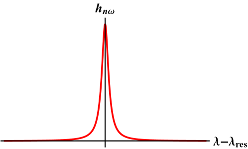
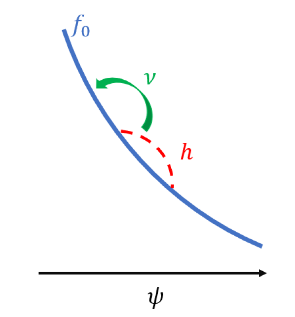
Our analysis of the transport equation (25) will reveal that the effect of the perturbations on particle motion is highest for particles which are in resonance with the mode, that is, those for which all terms on the left side of (25) vanish. If there were no collisionality, the effect of the perturbation drift [represented by the second term on the left side of (25)], on such resonant particles would diverge. So collisionality is necessary to resolve the singularity of the resonance.101010Here, we refer only to behavior existing within the equation we solve: a linearized drift kinetic equation with a perturbation of zero or real frequency. Physically, it is possible for other effects to resolve the resonance. For instance, resonant particles will dephase from the perturbation as they are moved by it, resulting in nonlinear resolution of the resonance through the formation of phase space islands. The addition of a small imaginary component to the perturbation frequency is also able to resolve the resonance. However, it is not clear that phase space island formation (in the absence of resonance overlap) or an imaginary component of the frequency provide the decorellation and dissipation necessary for transport. The relationship between these mechanisms and pitch angle collisions in resolving the resonance and in causing transport is an interesting avenue for future work. One possibility is that resonance resolution by these mechanisms is similar enough to the collisional resolution that fluxes calculated in this paper are valid in cases where collisional resolution is less important than other mechanisms. A small boundary layer of finite width in pitch angle space and velocity space will collisionally disrupt resonance with the mode, and the perturbed distribution function will vary sharply near this layer. Pitch angle scattering, represented by the second term in (9), rather than drag, is the important collisional behavior because the second derivative of the pitch angle scattering operator is stronger near the resonance boundary layer than the first derivative of the drag. A schematic picture of about a resonant location in pitch-angle space is given in figure 1. A possible physical interpretation of this resonance structure is that particles drift while resonant with the wave until they pitch angle scatter, giving rise to gradual diffusion (Helander & Sigmar, 2005).
This understanding yields a phenomenological estimate of the heat flux which should result from the transport being considered. The heat flux will be given by
| (32) |
with the alpha particle mass, a characteristic alpha resonant velocity, the fraction of particles that are resonant with the mode, the radial velocity caused by the perturbation, the time that a particle moves before becoming decorrelated by a collision (such that is the step a particle takes before becoming decorrelated). The fraction of particles affected by the mode is estimated from the width of the boundary layer representing the broadened resonance, given by balancing the left side of (25) (we use to include pitch angle dependence) with the pitch angle scattering part of the collision operator, (9),
| (33) |
with representing the coefficient of the second term of (9). [Note that the effect of the collision operator on the adiabatic component, , is negligible in comparison to the sharp variation of in the resonant boundary layer.] Thus, we have
| (34) |
The decorrelation time is given by , such that estimated flux is
| (35) |
Note that this flux is independent of the collision frequency because times is independent of the collision frequency. The role of the collisions is crucial to the transport, but collisionality does not appear in the final expression for the flux. Thus, in the following steps we use a Krook collision operator (Bhatnagar et al., 1954; Mynick, 1986), that is, an operator for which . The Krook operator is related to by [recall that the pitch angle scattering operator (9) depends on the second derivative of with respect to ]. We also ignore the effect of the collision operator on the adiabatic response because the sharp variation of is more important. Whenever collisions play a role in the calculation, they allow the convergence of a sum or resolve a singularity, actions which are not qualitatively sensitive to the full form of the collision operator.
4.3 Solution for with the Krook operator
Inserting the Krook operator and the form (30) into (25) reveals the equation to be solved for each :
| (36) |
Now, recall the variable , which characterizes the progression of particles along the magnetic field [see (107)]. Then, defining
| (37) |
(36) may be written
| (38) |
Here, we have chosen such that . The perturbed distribution function can then be found by integrating from , where , forward to the "present" time , with ,
| (39) |
Moving the exponential on the left side to the right side gives gives
| (40) |
The preceding expression represents the response of the plasma distribution to the presence of a perturbation of the tokamak fields. Next, we work to write this expression in a form which can be more easily evaluated and understood. The expression (40) can be split into contributions from each complete bounce (for a trapped particle) or poloidal transit (for a passing particle) of duration given by
| (41) |
such that
| (42) |
Note that at the trapped-passing boundary, the value of for a trapped particle is twice that for a passing particle. This complication will not affect the calculation that follows as velocity space integrations account for both signs of . Each portion of the integral may be modified with the change of variables , such that the entire integral reduces to the geometric series
| (43) |
This transformation requires that be the same (up to a factor of ) for each bounce or transit, which corresponds to the existence of periodicity. Trapped particles, which traverse the same values of on each orbit, automatically fulfill this condition, because is trivially the same for each bounce. Passing particles do not reverse course and traverse values of ranging from negative infinity to infinity. For them, the split is only possible when the particle motion is resonant with the wave, such that the contributions to transport from each transit are the same. When the particle is not in phase with the wave, however, (40) will approach zero integrated over the entire passing particle trajectory because of the rapid oscillation of the phase factor, unmitigated by periodicity. The following analysis is appropriate for all trapped particles and for resonant passing particles. The analysis will reveal in (46) onwards that transport comes from resonant particles only, such that the formulation is appropriate for all transport causing particles, passing and trapped.
Because of the small imaginary part provided by the collisionality, the series (43) is convergent and may be summed as
| (44) |
Expanding the denominator about its zeros using , with any integer, denoting the bounce or poloidal transit harmonic, gives
| (45) |
Alpha particles are in general very unlikely to pitch angle scatter because of their high energy. Thus, for nearly all particles, . In this limit, analogous to the limit that occurs in the plateau regime of neoclassical transport [see Helander & Sigmar (2005)], (45) approaches
| (46) |
Here, we have also split the integral in the exponential into two parts which both have limits at , where . In addition, we have introduced a delta function with a resonance function as its argument,
| (47) |
Only particles for which is very close to zero participate in transport, and the strength of pitch angle scattering is accentuated for them from the normal weak level. The sharp variation in between resonant particles and non-resonant particles (visible schematically in figure 1) leads to this accentuation.
These resonances, discussed at greater length in section 5.4, are bounce harmonic resonances, which occur when the mode frequency, the particle bounce frequency, and the tangential precession frequency resonate. Such resonances are familiar from treatments of neoclassical toroidal viscosity of bulk tokamak plasmas (Linsker & Boozer, 1982; Mynick, 1986; Park et al., 2009; Kim et al., 2013; Logan et al., 2013) and also appear in treatments of Alfvén eigenmode stability [see, for example, Borba & Kerner (1999)] and in single particle analyses of energetic particle transport by neoclassical tearing modes, another type of tokamak perturbation (Poli et al., 2008).
Finally, using (30) to obtain the full form of in terms of the unstarred coordinates gives the expression needed to form the heat flux,
| (48) |
5 Expression for flux
In this section, we show how to use the alpha distribution perturbation derived in the previous section to obtain the resulting alpha heat flux. This heat flux is the quantity of practical use in understanding and predicting tokamak discharges. In addition, we discuss key parts of the expression for this flux.
5.1 Setup of flux expression
To find the heat flux, the perturbation to the distribution function, , found in (48), is multiplied by the perturbed radial velocity that also results from the electromagnetic perturbation, .111111Some techniques for computing energetic particle transport, like the use of orbit following codes, focus only on the perturbed radial velocity. However, consistent consideration of both components is critical. An experimental demonstration of energetic particle transport caused by the product of the distribution function perturbation and the perturbed radial velocity is given in Nagaoka et al. (2008). Todo (2019) discusses these results and the importance of developing energetic particle transport theories that self consistently treat both of these components. The result is weighted by energy and integrated over the distribution function. Then, this quantity is averaged over the flux surface:
| (49) |
Here, the flux surface average is defined by
| (50) |
To enable analytic evaluation of the flux, we now adopt the following approximate expression for the strength of the axisymmetric magnetic field:
| (51) |
with (as introduced in section 2) small. Then,
| (52) |
The perturbation to the distribution function may be found in (48). The perturbed radial velocity may be read off from (22), giving
| (53) |
The flux has contributions from both trapped and passing particles, and will be evaluated in slightly different ways for each of these populations. In general, we illustrate the trapped particle techniques first, then modify them for passing particles later. One of the key differences between the trapped and the passing calculations is the treatment of the particle pitch angle (6). For trapped particles, integration in pitch angle is carried out in terms of the trapping variable , which is defined in terms of ,
| (54) |
This variable is defined such that, for a trapped particle, the angle of the turning point in the magnetic field (51) is given by . Deeply trapped particles have and barely trapped particles have . For passing particles, the analogous variable is
| (55) |
where a value of corresponds to a barely passing particle and a value of corresponds to a fully passing particle. [A pedagogical introduction to the trapping parameter can be found in Helander & Sigmar (2005).] With the definitions of (6) and (54) we can write the differential in (49) as
| (56) |
an equivalent expression in terms of holds for passing particles.
5.2 Discussion of synergistic transport from different
To evaluate the flux, (48), (52), (53), and (56) are inserted into (49). Note that the resulting flux includes sums over two different sets of and : one set for the perturbed distribution function (48), and one for the perturbed radial velocity (53). The complex quantities are written as their real equivalent and the integral is evaluated using the identities and , with and some phase and the Kronecker delta. Using these expressions, and stating the integral in terms of (107), we find for trapped particles
| (57) |
(the subscript indicates this is a trapped particle expression). Here, we have defined
| (58) |
and
| (59) |
Equivalent expressions in terms of instead of apply to passing particles. Consideration of (57) makes clear that there is no coupling between perturbation components of different toroidal mode numbers: the perturbed distribution function of one will not interact with the perturbed radial velocity of another . However, perturbations (or components of one perturbation) with the same toroidal mode number, but different poloidal mode numbers, can couple via the and terms. For perturbations of very different , these terms are highly oscillatory, such that the integral over will be small, as required by the Riemann-Lebesgue lemma. The flux resulting from this coupling approaches zero.
For perturbations of similar poloidal mode number, the coupling is significant and the perturbations cause synergistic transport in which the perturbed distribution function from one perturbation interacts with the perturbed drift velocity of the other to cause transport. Note that this synergistic transport will oscillate with time at a frequency equal to the difference between the two perturbations, as is typical for beat frequency phenomena. Transport at such a beat frequency has been observed experimentally in studies of transport in the presence of NTMs and field perturbations caused by resonant magnetic perturbations (Snicker et al., 2018). Evaluation of the flux for synergistic transport between poloidal harmonics requires numerical integration of (57). Furthermore, for the case of interaction between TAE harmonics with the same and , but different values of , the relationship (see table 2), ensures that the harmonics will have different values of and different radial profiles. The resulting rapid sinusoidal oscillations tend to reduce their contributions to transport. Thus, from here on, we evaluate the flux for a single perturbation, characterized by one value of , , and , with the knowledge that if a perturbation of a similar poloidal mode number is also present in the device at the same radial location, transport may be altered in a synergistic manner. We denote the single , , and flux .
5.3 Assumption of and final statement of flux
The flux is a function of flux ; the perturbation is also a function of this variable. However, , defined in (19), not , is a constant of the alpha particle’s motion, such that the alpha particle response is a function of . In the flux expression (57) appears only in the variable through the dependence of and on this quantity. Recalling (21) and (19), we have
| (60) |
[note that here we have provided in terms of both and shear , (4)]. Because is a function of , this quantity varies poloidally in a complicated manner. Such complication introduces significant challenge in the evaluation of the flux, in particular making the term that enforces resonance, , dependent on .
In this work, we thus choose to neglect the difference between and , leaving a detailed study of the effect of the difference between these quantities to future work. This simplification places constraints on the values of shear for which our work is valid. Because appears in the combination , we can compare to the other terms in this combination to develop the following condition for the validity of setting :
| (61) |
The degree of restriction that this condition places on the magnitude of the shear depends on the characteristics of the perturbation in question. For ripple, the condition is
| (62) |
a generous condition which allows the approximation to be valid even in the high shear regions near the tokamak edge where the ripple is important. For the TAE, the equivalent expression is
| (63) |
which, given the fairly high values of characterizing TAEs, is a more restrictive condition, though it should still hold in much of the low-shear core plasma where TAE activity is most common.
With the replacement , the outer integral in (57) can be commuted past . In addition, using (14), we can insert
| (64) |
into the definition of (28). (Recall that we have also taken .) This gives, for trapped particles,
| (65) |
The equivalent expression for passing particles is below, adding a subscript to make clear the expression refers to passing particles:
| (66) |
These expressions are central results for this paper and can be used to evaluate the alpha flux caused by a wide range of tokamak perturbations. In later sections, they will be applied to the flux resulting from ripple and TAEs as examples. Already, the expressions display clear and expected trends. That the flux is driven by the alpha density gradient is shown by the expression’s dependence on . That the flux increases with the perturbed amplitude squared is also clear. The following subsections examine the elements of these fluxes that remain opaque: the term , which enforces the resonance condition, and the term , which we refer to as a "phase factor."
5.4 Resonance condition
The flux expressions (65) and (66) include the delta function . This delta function enforces the resonance given in equation (47) and determines which particles are able to be transported by the mode and to contribute to the alpha flux. The expression for the resonance (47) can be evaluated to read [setting , as discussed in section 5.3]
| (67) |
where the bounce or transit time is defined in (41), is defined in (31), and the transit average drift is defined by
| (68) |
| Quantity | Trapped particles | Passing particles |
The terms in (67) can be evaluated for trapped and passing particles to give the expressions in terms of and or in Table 3.121212This evaluation follows from using the definitions of (107) and (26). In a magnetic field with strength described by (51), the parallel velocity appearing in and is . The changes of variable given later on in (69) and (76) are needed. The term in the flux expression thus relates the pitch angle and speed of particles that participate in transport and contribute to the flux.
5.5 Evaluation of phase factor
The term in (65) and (66) depends on integrals defined in (58) and (59). These integrals are evaluated along particle trajectories, which advance with (107). This complex term, which we refer to as a "phase factor," determines how effective a given resonance is at creating a perturbation to the alpha distribution function. In this subsection, we write the phase factor for trapped and passing particles in a form that can be integrated numerically or approximated.
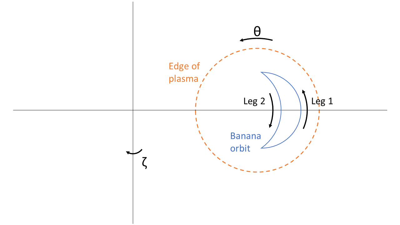
We begin with trapped particles. Trapped particles follow banana orbits, represented schematically in figure 2, with two legs on which the particle velocity is in opposite directions. Our evaluation assumes that the particle orbit is in resonance at a particular harmonic with the mode via (67). Only such resonant particles are able to contribute to the flux. The integrals in the phase factor are evaluated along each of these legs, which contribute in distinct ways that depend on and finite orbit effects to the overall phase factor.
We begin by introducing the variable , which is the following function of :
| (69) |
The definition of (54) can be used to show that the banana bounce points occur at , so that the use of standardizes the necessary integration. Now, to write and explicitly, we must write various quantities that appear in (107) or (37) in terms of . The parallel velocity in the magnetic field (51) is given by
| (70) |
where the last expression exploits that for trapped particles differs from by at most . The drift term appearing in , (26), is given by
| (71) |
We will also use to simplify our expressions.
| Expression | Value |
To make our presentation of the phase factor more compact, we define a set of expressions [,, , and ] given in table 4. Then, the contribution of the outer leg , which has velocity in the direction of positive , to (58) can be shown to equal (where we have again taken )
| (72) |
Meanwhile, the inner leg is given by
| (73) |
Here, our use of follows from the recognition that only particles which are in resonance according to (67) contribute to the flux, and that the quantity accumulates from and integrated over the entire orbit starting from . The inner leg value can be restated by applying the relationship and flipping the limits so they agree with those given for the outer leg:
| (74) |
Equivalent expressions hold for . Forming and evaluating the quantity reveals that the dependence on vanishes, as is to be expected given that this parameter depends on the parallel velocity evaluated at , an arbitrary location. Suppressing the dependence of , , and for compactness, the full phase factor reads
| (75) |
Though this expression is daunting, in practice many simplifications are possible. First, most modes have only a subset of , , and , and these quantities may be proportional to each other. In addition, it is sometimes possible to neglect some of the terms in the arguments of the cosine. The integrals can also be approximated in a variety of ways.
Passing particles are simpler to treat than trapped particles. For passing particles the variable is defined as:
| (76) |
Recalling the variable defined in (55), the parallel velocity in the magnetic field (51) for passing particles is given by
| (77) |
Note that can be very small for passing particles and thus cannot be set to 1 as it was for the trapped particles. For passing particles, the drift (26) is:
| (78) |
| Expression | Value |
We again define certain expressions to make the presentation of the phase factor more compact in Table 5. A passing particle orbit goes around the entire device, from to . Its is given by
| (79) |
An analogous expression holds for . Forming the sum of the two terms gives
| (80) |
Again, in practice this complicated expression can be simplified in a variety of ways.
6 Ripple flux
In this section, we consider the trapped and passing fluxes (65) and (66) for our first example perturbation: ripple, which has characteristic parameters described in table 2. We will find that the contribution of bounce harmonic resonances to the transport for this perturbation is small because is very high. Because of this realization, we do not provide an analytic expression for the flux.
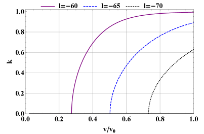
First, we consider the structure of the resonances between alphas and ripple in a tokamak with parameters given in table 1. These are plotted in figures 3, 4, and 5, for trapped particles with , for passing particles with , and for passing particles with . Specifically, these figures show, for typical values of , the values of and (or ) for which and the delta function in (65) or (66) has support. The lines in the plot identify the areas of phase space which could contribute to transport. The resonance structure is only shown up to the alpha birth velocity because alpha particles are unable to interact with perturbations through resonances above this velocity.
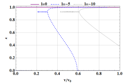
Trapped ripple resonances are shown in figure 3. Trapped resonances can occur at most values of for negative values of of intermediate magnitude ( and are shown in the plot). An alpha particle is born at and a specific value of . As the particle slows down, it will move left along the -axis while maintaining the same value of . During this process, the alpha interacts with the perturbation when it crosses a resonance line. Note that in this case, the lines representing some harmonics are multivalued in at some velocities. This simply means that at that velocity, multiple pitch angles are able to interact with the mode.
A series of resonances near the trapped-passing boundary () also exists. These include parts of harmonics and all of ,131313Note that the resonance is so close to because we selected as an example parameter (see table 2). For lower values of shear, the resonance occurs at lower values of and does not suffer from the resonance crowding described in this paragraph. However, ripple does tend to be strongest in regions of high shear, so is an appropriate example value. shown in the plot. There are also several more resonances, corresponding to , at , which are not displayed in the plot for clarity. Because the resonances at are very close to each other in pitch angle and very near to the trapped-passing boundary layer where other boundary layer physics enters (Catto, 2018), the use of the Krook operator to represent pitch angle scattering is not well justified, making the treatment in this paper unsatisfactory for this region. A more elaborate boundary layer theory is necessary to satisfactorily treat these resonances, so in this paper we focus on the lower parts of the trapped resonances with .
For passing particles, shown in figures 4 and 5, which have in (67), the large value of characterizing ripple means that resonances occur at values of of large magnitude. At alpha birth (the right side of the plot), particles near trapped-passing boundary () resonate with ripple, while at lower speeds, freely passing particles (small ) resonate with ripple.
After understanding the resonance structure, the next step in the evaluation of flux is to consider the phase factor , discussed in section 5.5. However, this phase factor is very small for ripple resonances. As an example, figure 6 shows the numerically evaluated phase factor for the trapped harmonic displayed in figure 3. Specifically, this plot shows the quantity (75) as a function of , where (75) is numerically evaluated at the value of that is resonant at that value of . The small values of the phase factor evident in figure 6 are typical of those for all ripple resonances.
These small values result from the highly oscillatory nature of ripple phase factor, which we demonstrate using the original definition of , (58), and of , (59). In particular, the argument of the sinusoids in (58) and (59) can be roughly approximated by
| (81) |
for values of and satisfying the resonance condition. [Here, is defined in (68).] To obtain this expression, we have considered the definition of , (37), and inserted , , and , as appropriate for ripple. Then, we have treated as though it were constant and independent of [we note that a similar approximation was used to evaluate related phase factors in previous studies of the effect of non-axisymmetries on bulk plasma (Park et al., 2009)]. Then, the resonance condition (67) can be applied to (81) to reveal
| (82) |
(For the passing expression, we have taken the additional approximation .) These expressions indicate that the arguments of the sinusoids in (58) and (59) change very quickly if, for trapped particles, is large or, for passing particles, is large. The corresponding phase integrands in the phase factor are highly oscillatory. The Riemann-Lebesgue lemma states that such integrals must approach zero as for trapped particles and for passing particles.
Ripple is characterized by . Then, consideration of the harmonics characterizing resonances that exist in a typical tokamak, illustrated in figures 3, 4, and 5, reveals that for trapped particles is always large and for passing particles is large.141414The reader might ask if it is possible to construct any tokamak in which is small for trapped particle ripple resonances and is small for passing particle ripple resonances. For trapped particles, this would require in (67). This reduces to the requirement , which requires unrealistically small machine size or magnetic field. A similar condition is found for passing particles. Based on Eq. (82) and the discussion in the previous pragraph, this means the phase factors for ripple perturbations are extremely small, as exemplified in figure 6.
With such a small phase factor, the flux described by (65) and (66) is negligible. Therefore, bounce harmonic resonant transport is very weak for ripple perturbations and will not create noticeable alpha heat flux. Alpha transport from ripple may, however, occur via other mechanisms, including stochastic ripple diffusion and ripple trapping (Goldston et al., 1981; White et al., 1995; Catto, 2018).151515Some of these mechanisms are collisionless. One might at first expect collisionless processes to be unimportant in steady state, where refilling of loss regions is necessary for sustained transport. However, alpha particles are continuously introduced to the tokamak via fusion, which serves to refill loss regions. Therefore, consideration of collisionless processes in tokamak design is critical to achieving satisfactory steady state behavior. In addition, further work should consider the impact of externally-applied 3D magnetic field perturbations, such as those used for ELM control, which could cause significant alpha transport (Sanchis et al., 2018).
7 TAE flux
In this section, we evaluate the trapped and passing fluxes (65) and (66) for the example case of the TAE, which has characteristic parameters described in table 2. We find that the TAE can cause significant alpha heat flux, and develop a constraint the TAE amplitude must obey to prevent significant alpha depletion. At the end of the section, we develop a simple saturation model for TAE. This model suggests that TAEs in SPARC-like tokamaks will saturate below the level at which bounce harmonic resonant transport can cause significant alpha depletion. However, saturation amplitudes above those suggested by our model, but within computational and experimental experience, could cause depletion.
7.1 Evaluation of flux

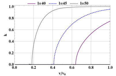
The resonance structures for the TAE are shown in figures 7, 8, and 9. Trapped particles are able to resonate with the TAE at low values of the harmonic , as seen in figure 7. Near the alpha particle birth speed (the right edge of the plot) the mode resonates with a small subset of pitch angles nearer the trapped-passing boundary (). As the alpha particles slow down (moving left along the x-axis), a wider range of pitch angles can resonate with the mode. For a given value of , lower values of are able to resonate with higher speed particles.
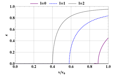
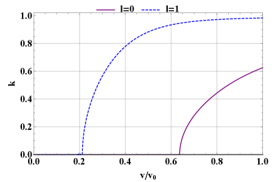
Passing particle resonances (with both and ) with the TAE are similar, with alpha particles near birth resonating with barely passing particles and those that have slowed down resonating at a wider variety of pitch angles. These resonance structures can be seen in figures 8 and 9. Again, lower values of tend to resonate with higher velocity particles for a given value of . As the drift is negative, an resonance is only possible for , but we will soon find the transport associated with this sign of is very small. Note that fully passing particles (with ) resonate at the Alfvén speed and one third of the Alfvén speed. This aligns with the resonance structure described in simplified treatments of TAE resonance which focus on freely passing particles (Heidbrink, 2008; Betti & Freidberg, 1992).
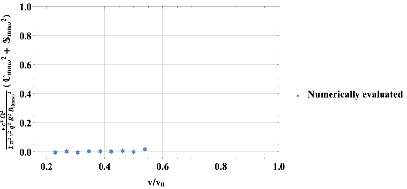
Now, we move to the evaluation of the TAE flux, starting with trapped particles. Again, this procedure begins with consideration of the phase factor (75). Full evaluation of this quantity must be done numerically. However, a tolerable approximation of its value can be made for low values of . At low for typical TAE parameters, the dominant term in the sinusoids of the phase factor is the finite orbit width term . This can be verified numerically. After neglecting and , the terms in the phase factor which are proportional to can be neglected as higher order in . Then, the terms (for even ) and (for odd ) can be written in terms of Bessel functions using the Bessel generating function . Here, represents the Bessel function of the first kind of order . Higher values of in the sum are more oscillatory and do not contribute much to the phase factor integral. So, only the lowest are maintained. This process gives:
| (83) |
The approximation in (83) is compared to a full numerical evaluation of (75) for , , and in figure 10. This comparison shows that, although the approximation is not exact, it captures key trends in the phase factor for low values of . The approximation is less good for higher values of , where becomes more important and cannot be neglected.
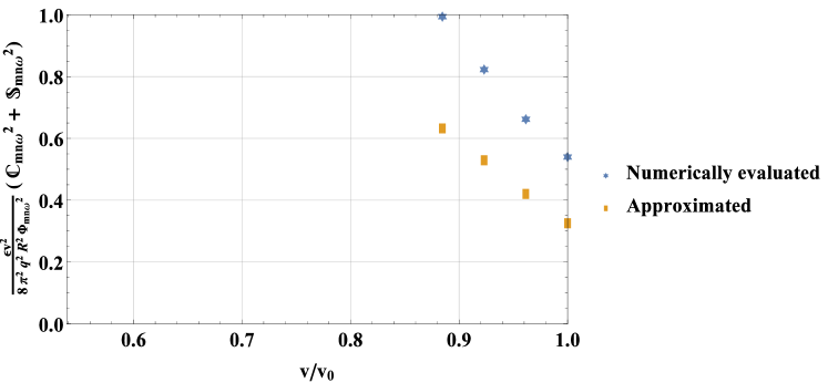
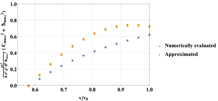
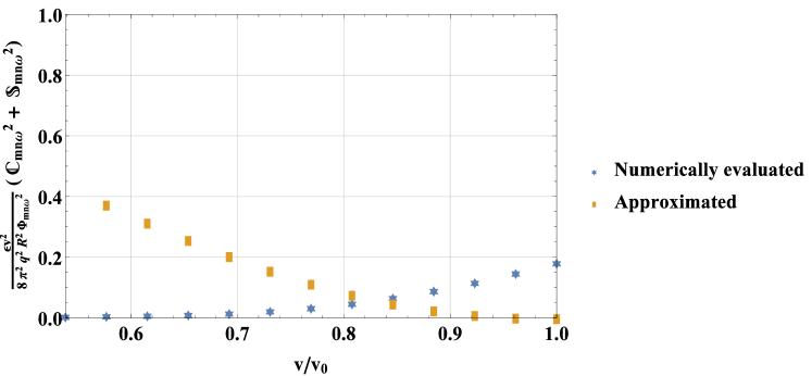
However, higher values of will have minimal contribution to the flux for three reasons. First, the resonance structures in figures 7, 8, and 9 make clear that, for a given value of , higher values of correspond to lower values of . These values of contribute less heat flux, which depends on . Second, the second term in , which appears in the flux expression (65), scales with velocity like [as we will see later on in (85)], further reducing the contribution of lower velocities to the flux. Finally, similar arguments to those used in the consideration of the ripple phase factor show that the sinusoids in the phase factor will become highly oscillatory for high values of , such that the value of the phase factor must shrink by the Riemann-Lebesgue lemma. This can be verified computationally. In figure 10, the phase factor for is already smaller than for and , which is an example of this effect. Because higher harmonics have such small contributions to the flux, in this section we compute the contributions from only.
We now proceed with the evaluation of (65). To lowest order in , the denominator of (65) is 1. The delta function enforcing the resonance is , with as evaluated in (67) with for trapped particles. This delta function is used to evaluate the velocity integral, recalling the general property that
| (84) |
for any function with roots . Furthermore, we can write that
| (85) |
with the alpha scale length defined in (7). For typical values of , ; inserting this scaling and the resonant value of where gives that
| (86) |
such that may be set to to lowest order in (at higher values of than those considered here, where the resonant becomes very small for many values of , this replacement would not be appropriate). Then, the contribution to the flux from each reduces to a fairly compact integral over . This integral is different for even and odd:
| (87) |
Here, is the resonant velocity at which . The value of in resonance at the birth velocity is called , i.e., using (67) and table 3,
| (88) |
The integrals in (87) can easily be evaluated numerically for specific values of the relevant parameters.
To obtain a closed expression, we now make another set of approximations for the values of . For , is low, and the resonance condition (88) is expanded about to and then solved for . For higher values of , with higher values of , different approximations are used. The quantity vanishes at the point and is small near that value. Resonances with have values of in this region. For , we can simply approximate with this value. For resonances of higher , we can neglect the term proportional to in the resonance condition (88). Also, we make the replacement in the remaining terms [this is the limit of as ]. This process gives, where we have inserted to simplify the expressions,161616The approximation, and the fluxes that follow from it, only provide physical values when . When device Alfvén speed violates this inequality, the resonance vanishes, and its contribution should be neglected.
| (89) |
The integrands can be expanded about to lowest non-trivial order in [ for even and for odd]. Prior to making the expansion for odd , the velocity in the argument of is replaced with the birth velocity. Comparison of the resulting approximate integrands to the numerically evaluated integrands shows that the approximations are good throughout the integration interval. Then, we calculate
| (90) |
where is a parameter given in table 6 for the most important low harmonics.
| Expression | Value |
This expression, giving the trapped particle alpha heat flux from a TAE of a given magnitude, is a central result of this paper. For the example parameters in this paper, .
Now, we consider passing particles, with flux given by the expression in (66). The first step is to approximate the phase factor (80). The dominant term in the phase factor sinusoids is again . However, it is not possible to use the Bessel generating function for the passing particles, so instead we simply take and . Then the phase factor becomes, for even or odd,
| (91) |
This approximation is compared to the full numerical evaluation of the phase factor in table 7.
![[Uncaptioned image]](https://cdn.awesomepapers.org/papers/886d0377-79d7-4a05-b7f9-e72b60c9f3ff/x12.png) No resonance
No resonance
![[Uncaptioned image]](https://cdn.awesomepapers.org/papers/886d0377-79d7-4a05-b7f9-e72b60c9f3ff/x13.png)
![[Uncaptioned image]](https://cdn.awesomepapers.org/papers/886d0377-79d7-4a05-b7f9-e72b60c9f3ff/x14.png) Very low contribution to flux
Very low contribution to flux
![[Uncaptioned image]](https://cdn.awesomepapers.org/papers/886d0377-79d7-4a05-b7f9-e72b60c9f3ff/x15.png)
Notably, the phase factor is very small for in both the numerically evaluated and the approximated forms. This results from the cancellation between the contribution to the phase factor from the electric potential and that from the parallel vector potential. Thus, moving forward we evaluate only the contribution from .
The denominator in (66) cannot be set to as it was for the evaluation of the trapped flux (65); however, the delta function is applied in the same way as for the trapped particles, using (67), and is again to lowest order in . We set because, as discussed previously, this is the only significant contribution to the flux. Then the integral to be evaluated is
| (92) |
where is the resonant velocity at which . The upper limit of integration is the value of in resonance at the birth velocity , which can be found for each value of using (67) and the passing quantities in table 3.
For , a good approximation for is found from expanding the resonance condition about to . In contrast, for , a good approximation is found by expanding about to . This process gives, with used to simplify the expressions:
| (93) |
The integrand can again be expanded about to lowest non-trivial order in . Then, we find, where we have inserted
| (94) |
where are parameters given in table 8. Again, we include only harmonics . Higher harmonics have small contribution to the flux. This expression, giving the passing particle alpha heat flux from a TAE of a given magnitude, is another central result of this paper. For the example parameters in this paper, . The passing flux is larger than the trapped flux. This results from multiple factors. For instance, there are more passing particles than trapped particles in the isotropic alpha population. Also, the passing phase factor tends to be larger than the trapped phase factor.
| Expression | Value |
The expressions for the trapped, (90), and passing, (94), fluxes can be compared to the phenomenological flux, (35). In particular, for the trapped flux, (90), setting and reproduces the dependencies seen in (90). For the passing flux, setting , and making the same replacement as for the trapped for the radial velocity reproduces the dependencies seen in (94). As intuition suggests, the heat flux scales with the square of the perturbation amplitude, , and increases with the periodicity of the mode, .
7.2 Interpretation of flux and development of saturation condition
The magnitude of the alpha flux caused by the TAE is understood by comparing the rate of the diffusion it causes to the rate of slowing down. Slowing down (described in appendix A) removes alpha particles from the energetic population and transfers their energy to the local bulk plasma, leaving the alpha particles as helium ash. So, with the diffusion coefficient describing the TAE flux and the device minor radius, if
| (95) |
TAE diffusion is weak and does not remove alpha particles before they can give their energy to the background plasma and transition to ash. When
| (96) |
TAE diffusion is very strong. It would be capable of diffusing alpha particles across the whole poloidal tokamak cross section (with an area that scales as ) in a slowing down time if mode activity of similar strength existed across that area. (Note that the width of an individual mode is significantly smaller than .) At this level, alpha particles diffuse sufficiently fast to cause significant modification to the alpha heat deposition profile. (At this point the perturbative approach used in this paper becomes inappropriate. For losses at this level, a quasilinear treatment which retains the radial flux losses in (102) for is needed.) The diffusion coefficient is related to the flux by
| (97) |
such that the condition for avoiding strong TAE diffusion, (95), becomes
| (98) |
for trapped particles and
| (99) |
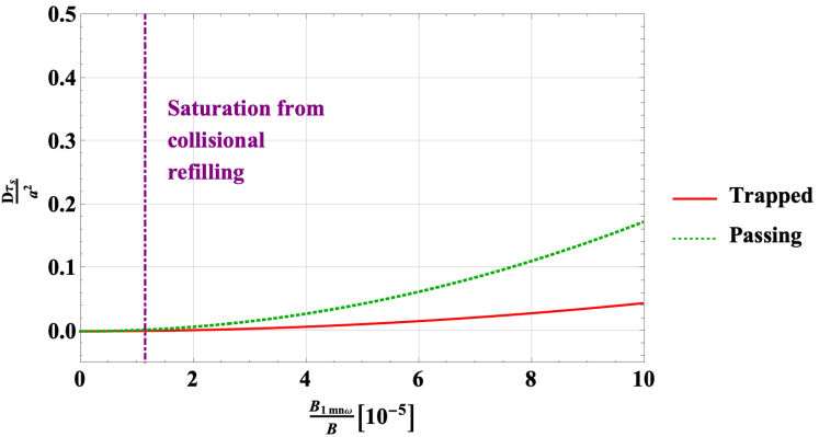
for passing particles. Here, we have stated the flux in terms of the strength of the perturbed magnetic field, , which is more commonly seen in the literature than . In addition, we have used . For fixed tokamak equilibrium parameters and fixed radial location , these conditions constrain the maximum amplitude for the mode to avoid serious alpha depletion. We plot the value of as a function of the normalized mode amplitude, , in figure 11.
Understanding how this constraint compares to typical TAE amplitudes requires a rough estimate for mode saturation. We now develop such an estimate. TAE saturation has been estimated using a variety of methods. Some works balance the linear growth rate of the instability with the rate at which particles get trapped by the wave and flatten the gradient driving the instability, sometimes including collisions which restore the original gradient (Wu & White, 1994; Fu & Park, 1995; Wang & Briguglio, 2016; Zhou & White, 2016; Todo, 2019). Other works consider the effects of zonal flows and nonlinear mode couplings (Spong et al., 1994; Chen & Zonca, 2012). Our technique for estimating saturation is similar to the first of these approaches in that it also considers TAE drive reduction due to the flattening of the alpha gradient and collisional refilling of this gradient. However, we consider the removal of the drive to be due to flattening, rather than due to particle trapping.
The mechanism of saturation is represented schematically in figure 12.
As the TAE grows, the non-adiabatic particle response reduces the alpha gradient responsible for mode drive. However, collisions concurrently act to restore the original particle gradient by counteracting this flattening. The balance of these processes results in mode saturation. (If the original drive were not restored fast enough by collisions, and the mode amplitude would shrink, while if it were restored faster than it was reduced, and mode amplitude would grow.) Mathematically, this balance is stated
| (100) |
The left side is the rate at which the drive for , , is reduced by . The right side, , is the rate at which the original drive is restored by collisions.
This saturation condition can be evaluated in two different limits. The first, low collisionality, limit occurs when , with given by (34). (This expression is for trapped particles; the equivalent passing expression is in terms of .) The second, high collisionality, limit occurs when , with given by the value for the TAE given in table 2. The transition between the two limits occurs when . Inserting , with given by (34) with , and reveals the saturated amplitude of the TAE:
| (101) |
Here, [from the second term in the collision operator (9)]. Similar scalings of saturated amplitude with collisionality are found elsewhere in the literature (Berk et al., 1992; Slaby et al., 2018; White et al., 2019). For the parameters used in tables 1 and 2, the low collisionality limit is appropriate, and gives an amplitude of roughly . This saturation estimate is comfortably below the stochastic threshold given in Berk et al. (1992), making it consistent with our assumption throughout the paper that the TAE amplitude is below the threshold for stochasticity.
Saturated AE amplitudes observed experimentally (Nazikian et al., 1997; Van Zeeland et al., 2006; Fasoli et al., 1997) and predicted computationally (Fitzgerald et al., 2016) or analytically (Zonca et al., 1995) using other models have found amplitudes ranging from to across a wide range of machine parameters and types of energetic particle populations; in extreme cases, amplitudes of have even been found (Todo et al., 2003). Thus, our estimated amplitude is at the bottom of the range typically found in the literature.
The expected saturated amplitude at the example parameters used in this paper, , is indicated on the plot of diffusion strength, figure 11, with a purple dash-dotted line, revealing that at this amplitude, is small for both the trapped and the passing populations. At this amplitude, significant redistribution of alphas due to this TAE is not expected, though some localized alpha gradient flattening may occur. (In addition, synergistic action with overlapping modes of different and could change the transport; since TAEs consist of coupled poloidal harmonics, this change is likely to occur.) An increase in saturated amplitude from the level predicted in our simplified model, but still within the range commonly seen in the literature, could lead to significant redistribution. This significant activity is especially likely for the passing population.
8 Conclusion
This work has developed the drift kinetic theory of transport that results from resonance between alpha particle motion and a perturbation to the tokamak magnetic and electric fields. The theory allows the calculation of the alpha particle heat flux of trapped and passing particles that results from these perturbations, (65) and (66). These expressions are examined for two specific perturbations: ripple and TAE. For ripple, this mechanism causes negligible alpha particle transport, as discussed in section 6. For TAE, the mechanism causes significant heat flux [given by (90) for trapped particles and (94) for passing particles] which allows the development of constraints on TAE amplitude to avoid significant depletion of the alpha population [given by (98) for trapped particles and (99) for passing particles]. A simple saturation condition suggests that the TAE amplitude in a tokamak scenario similar to that which might occur in the next generation tokamak SPARC is below this limit. This is a reassuring conclusion because significant alpha transport due to TAEs has the potential to seriously impair tokamak operation. However, the presence of other mechanisms for TAE transport [such as the removal of alphas due to their being born in stochastic regions as considered further in Sigmar et al. (1992) and Collins et al. (2016)] and the precedent for larger saturation amplitude in the experimental and analytical literature suggest that caution is still important.
Our expressions for the radial heat transport are independent of the collision frequency even though each wave-particle resonance path in velocity space is at the center of a narrow collisional boundary layer. Indeed, our resonant plateau model is reminiscent of quasilinear treatments in the sense that the narrow collisional boundary layer results in and gives meaning to the delta function behavior that removes the collision frequency when the alpha heat flux is evaluated [see the diffusive limit in Duarte et al. (2019) and the pitch angle scattering treatment of Catto (2020)]. Our expressions for the alpha heat fluxes are most appropriate when the phase space islands about the wave-particle resonance curves do not overlap. However, the expressions may remain reasonable even as the islands begin to overlap provided the TAE amplitude remains below the threshold for full stochasticity.
Avenues for future work based on this paper fall into three categories: analytical, numerical, and experimental. On the analytical front, future work should adapt and improve the formalism developed in this paper so that it can be used to study other species of energetic particle, which have more complicated distribution functions than the alpha distribution function. This will enable comparison of this model’s predictions to current experiments without alpha particles. In addition, analytical work could focus on the calculation of the flux for perturbations for which the approximation , discussed in section 5.3, is not possible. This includes the neoclassical tearing mode (La Haye, 2006), for which , making it necessary to avoid the condition in (61). Evaluation of the flux from such perturbations requires modified techniques. Finally, additional analytical work should consider adaptation of the techniques developed in this paper for use with a more precise collision operator than the Krook operator. This would allow the study of resonances, like some of the ripple resonances discussed in section 6, which are spaced too closely for the Krook operator to be appropriate.
On the numerical front, effort should be made to determine the relative importance of the transport mechanisms studied in this paper and those that are the focus of other works on energetic particle transport. Other mechanisms include overlapping phase space islands from different resonances, the transfer of alpha particles across topological boundaries (for example, the trapped-passing boundary), and convective transport which occurs when an alpha particle near the edge stays in phase with a perturbation without scattering until it leaves the device (Heidbrink, 2008). Simulations of alpha transport due to tokamak perturbations using the orbit following codes discussed in the introduction can be examined to distinguish transport resulting from these mechanisms. Such simulations should take care to properly resolve the boundary layer around the resonant velocity and pitch angles. We note that collisional boundary layer behavior was recently observed in White et al. (2019), but was attributed to an alternate mechanism.
On the experimental front, the predictions in this paper should be validated against estimates of alpha particle flux from measurements of actual experiments. Such validation will be possible in next generation experiments which are dominantly alpha heated, like SPARC and ITER, and may be possible in "afterglow" scenarios of experiments with some alpha heating, like the forthcoming JET DT campaign. [Afterglow scenarios, discussed in Sharapov et al. (1999), occur when external heating is suddenly turned off in order to transiently observe alpha particle effects.] If the formalism in this paper is adapted to distributions typical of energetic particles resulting from ICRF or beams, which are common in current day experiments, precise comparison to current experiments is possible. Already, current experimental measurements can be examined for evidence of general trends suggested by our work. For instance, part of the energetic particle flux resulting from energetic particle mode perturbations has been nicely demonstrated to scale with mode amplitude squared in Nagaoka et al. (2008). This agrees with our predictions.
The authors thank Steven Scott, Ryan Sweeney, Abhay Ram, Ian Abel, Ian Hutchinson, Eero Hirvijoki, Antti Snicker, Konsta Särkimäki, Paulo Rodrigues, Earl Marmar, Felix Parra, Iván Calvo, Vinícius Duarte, Lucio Milanese, and Martin Greenwald for helpful conversations. The authors are especially grateful to Nuno Loureiro for suggesting P.J.C. become involved in the problem and for several insightful suggestions. The authors acknowledge support from the National Science Foundation Graduate Research Fellowship under Grant No. DGE-1122374, support from US Department of Energy award DE-FG02-91ER54109, and support from the Bezos Membership at the Institute for Advanced Study.
Appendix A Derivation of equilibrium alpha particle slowing down distribution
The equilibrium energetic alpha distribution, , is determined by (8) in the unperturbed magnetic field (2):
| (102) |
This expression is solved by separating its terms by size and solving for the corresponding size terms in the distribution function, with . The largest term in the unperturbed drift kinetic equation (102) is the streaming term, so that
| (103) |
This equation shows is a flux function, i.e.,
| (104) |
The next order expression includes the drift term (which can be shown to be small compared to the streaming term by the poloidal alpha gyroradius over the perpendicular scale length of ), the collision operator (which is small by the connection length over the alpha mean free path), and the source term (which must be the same size as the collision operator for alpha particles to slow down before they are lost due to other processes). This expression reads
| (105) |
Because spatially depends only on , we have that
| (106) |
where the final expression can be derived as explained in equation (8.14) of Helander & Sigmar (2005).
We define the variable characterizing the progression of particles along the magnetic field,
| (107) |
with a unit of distance along the magnetic field. Integration over over a closed orbit annihilates the left side of (105), giving
| (108) |
Because is not a function of [recall (104)], the integrand on the right side must be identically zero. Enforcing this condition using (9) (note that alphas are born isotropically, so only the first term in is important here) gives the slowing down distribution,
| (109) |
Insertion of the slowing down distribution into (105) gives that
| (110) |
which shows that is a flux function. Evaluation of the drift kinetic equation to the next order allows the derivation of neoclassical alpha transport driven by the term , as discussed in Catto (2018). However, in this paper we focus on transport caused by perturbations and take that . This means that we assume
| (111) |
which is equivalent to stating , with the alpha particle scale length defined in (7).
References
- Berk et al. (1995) Berk, H.L., Breizman, B.N., Fitzpatrick, J. & Wong, H.V. 1995 Line broadened quasi-linear burst model [fusion plasma]. Nuclear Fusion 35 (12), 1661.
- Berk et al. (1992) Berk, H.L., Breizman, B.N. & Ye, H. 1992 Scenarios for the nonlinear evolution of alpha-particle-induced Alfvén wave instability. Physical Review Letters 68 (24), 3563.
- Betti & Freidberg (1992) Betti, R. & Freidberg, J.P. 1992 Stability of Alfvén gap modes in burning plasmas. Physics of Fluids B: Plasma Physics 4 (6), 1465–1474.
- Betti & Freidberg (1993) Betti, R. & Freidberg, J.P. 1993 Destabilization of the internal kink by energetic-circulating ions. Physical Review Letters 70 (22), 3428.
- Bhatnagar et al. (1954) Bhatnagar, P.L., Gross, E.P. & Krook, M. 1954 A model for collision processes in gases. I. small amplitude processes in charged and neutral one-component systems. Physical Review 94 (3), 511.
- Borba & Kerner (1999) Borba, D. & Kerner, W. 1999 CASTOR-K: Stability analysis of Alfvén eigenmodes in the presence of energetic ions in tokamaks. Journal of Computational Physics 153 (1), 101–138.
- Breizman & Sharapov (1995) Breizman, B.N. & Sharapov, S.E. 1995 Energetic particle drive for toroidicity-induced Alfvén eigenmodes and kinetic toroidicity-induced Alfvén eigenmodes in a low-shear tokamak. Plasma Physics and Controlled Fusion 37 (10), 1057.
- Calvo et al. (2017) Calvo, I., Parra, F.I., Velasco, J. Luis & Alonso, J.A. 2017 The effect of tangential drifts on neoclassical transport in stellarators close to omnigeneity. Plasma Physics and Controlled Fusion 59 (5), 055014.
- Catto (2018) Catto, P.J. 2018 Ripple modifications to alpha transport in tokamaks. Journal of Plasma Physics 84 (5).
- Catto (2019a) Catto, P.J. 2019a Collisional alpha transport in a weakly non-quasisymmetric stellarator magnetic field. Journal of Plasma Physics 85 (2).
- Catto (2019b) Catto, P.J. 2019b Collisional alpha transport in a weakly rippled magnetic field. Journal of Plasma Physics 85 (2).
- Catto (2020) Catto, P.J. 2020 Collisional effects on resonant particles in quasilinear theory. Journal of Plasma Physics 86 (3).
- Chen & Zonca (2012) Chen, L. & Zonca, F. 2012 Nonlinear excitations of zonal structures by toroidal Alfvén eigenmodes. Physical Review Letters 109 (14), 145002.
- Cheng & Chance (1986) Cheng, C.Z. & Chance, M.S. 1986 Low-n shear Alfvén spectra in axisymmetric toroidal plasmas. The Physics of Fluids 29 (11), 3695–3701.
- Collins et al. (2016) Collins, C.S., Heidbrink, W.W., Austin, M.E., Kramer, G.J., Pace, D.C., Petty, C.C., Stagner, L., Van Zeeland, M.A., White, R.B., Zhu, Y.B. & others 2016 Observation of critical-gradient behavior in Alfvén-eigenmode-induced fast-ion transport. Physical Review Letters 116 (9), 095001.
- Collins et al. (2017) Collins, C.S., Heidbrink, W.W., Podestà, M., White, R.B., Kramer, G.J., Pace, D.C., Petty, C.C., Stagner, L., Van Zeeland, M.A., Zhu, Y.B. & others 2017 Phase-space dependent critical gradient behavior of fast-ion transport due to Alfvén eigenmodes. Nuclear Fusion 57 (8), 086005.
- Cordey (1976) Cordey, JG 1976 Effects of particle trapping on the slowing-down of fast ions in a toroidal plasma. Nuclear Fusion 16 (3), 499.
- Creely et al. (2020) Creely, A.J. & others 2020 Overview of the SPARC tokamak. Journal of Plasma Physics 86 (5).
- Duarte et al. (2019) Duarte, V.N., Gorelenkov, N.N., White, R.B. & Berk, H.L. 2019 Collisional resonance function in discrete-resonance quasilinear plasma systems. Physics of Plasmas 26 (12), 120701.
- Fasoli et al. (1997) Fasoli, A., Borba, D., Gormezano, C., Heeter, R., Jaun, A., Jacquinot, J., Kerner, W., King, Q., Lister, J.B., Sharapov, S. & others 1997 Alfvén eigenmode experiments in tokamaks and stellarators. Plasma Physics and Controlled Fusion 39 (12B), B287.
- Fitzgerald et al. (2016) Fitzgerald, M., Sharapov, S.E., Rodrigues, P. & Borba, D. 2016 Predictive nonlinear studies of TAE-induced alpha-particle transport in the ITER baseline scenario. Nuclear Fusion 56 (11), 112010.
- Fu & Cheng (1992) Fu, G.Y. & Cheng, C.Z. 1992 Excitation of high-n toroidicity-induced shear Alfvén eigenmodes by energetic particles and fusion alpha particles in tokamaks. Physics of Fluids B: Plasma Physics 4 (11), 3722–3734.
- Fu & Park (1995) Fu, G.Y. & Park, W. 1995 Nonlinear hybrid simulation of the toroidicity-induced Alfvén eigenmode. Physical Review Letters 74 (9), 1594.
- Fu & Van Dam (1989) Fu, G.Y. & Van Dam, J.W. 1989 Excitation of the toroidicity-induced shear Alfvén eigenmode by fusion alpha particles in an ignited tokamak. Physics of Fluids B: Plasma Physics 1 (10), 1949–1952.
- Fülöp et al. (1996) Fülöp, T., Lisak, M., Kolesnichenko, Y. I. & Anderson, D. 1996 Finite orbit width stabilizing effect on toroidal Alfvén eigenmodes excited by passing and trapped energetic ions. Plasma Physics and Controlled Fusion 38 (6), 811.
- Goldston et al. (1981) Goldston, R.J., White, R.B. & Boozer, A.H. 1981 Confinement of high-energy trapped particles in tokamaks. Physical Review Letters 47 (9), 647.
- Hazeltine (1973) Hazeltine, R.D. 1973 Recursive derivation of drift-kinetic equation. Plasma Physics 15 (1), 77.
- Heidbrink (2002) Heidbrink, W.W. 2002 Alpha particle physics in a tokamak burning plasma experiment. Physics of Plasmas 9 (5), 2113–2119.
- Heidbrink (2008) Heidbrink, W.W. 2008 Basic physics of Alfvén instabilities driven by energetic particles in toroidally confined plasmas. Physics of Plasmas 15 (5), 055501.
- Heidbrink & White (2020) Heidbrink, W.W. & White, R.B. 2020 Mechanisms of energetic-particle transport in magnetically confined plasmas. Physics of Plasmas 27 (3), 030901.
- Helander & Sigmar (2005) Helander, P. & Sigmar, D.J. 2005 Collisional transport in magnetized plasmas, , vol. 4. Cambridge University Press.
- Hirvijoki et al. (2014) Hirvijoki, E., Asunta, O., Koskela, T., Kurki-Suonio, T., Miettunen, J., Sipilä, S., Snicker, A. & Äkäslompolo, S. 2014 ASCOT: Solving the kinetic equation of minority particle species in tokamak plasmas. Computer Physics Communications 185 (4), 1310–1321.
- Hirvijoki et al. (2012) Hirvijoki, E., Snicker, A., Korpilo, T., Lauber, P., Poli, E., Schneller, M. & Kurki-Suonio, T. 2012 Alfvén eigenmodes and neoclassical tearing modes for orbit-following implementations. Computer Physics Communications 183 (12), 2589–2593.
- Ikeda et al. (2007) Ikeda, K. & others 2007 Progress in the ITER physics basis. Nuclear Fusion 47 (6).
- Kim et al. (2013) Kim, K., Park, J.K. & Boozer, A.H. 2013 Numerical verification of bounce-harmonic resonances in neoclassical toroidal viscosity for tokamaks. Physical Review Letters 110 (18), 185004.
- Kurki-Suonio et al. (2009) Kurki-Suonio, T., Asunta, O., Hellsten, T., Hynönen, V., Johnson, T., Koskela, T., Lönnroth, J., Parail, V., Roccella, M., Saibene, G. & others 2009 Ascot simulations of fast ion power loads to the plasma-facing components in iter. Nuclear Fusion 49 (9), 095001.
- La Haye (2006) La Haye, R.J. 2006 Neoclassical tearing modes and their control. Physics of Plasmas 13 (5), 055501.
- Linsker & Boozer (1982) Linsker, R. & Boozer, A.H. 1982 Banana drift transport in tokamaks with ripple. The Physics of Fluids 25 (1), 143–147.
- Logan et al. (2013) Logan, N.C., Park, J.K., Kim, K., Wang, Z. & Berkery, J.W. 2013 Neoclassical toroidal viscosity in perturbed equilibria with general tokamak geometry. Physics of Plasmas 20 (12), 122507.
- Mynick (1986) Mynick, H.E. 1986 Generalized banana-drift transport. Nuclear Fusion 26 (4), 491.
- Nagaoka et al. (2008) Nagaoka, K., Isobe, M., Toi, K., Shimizu, A., Fujisawa, A., Ohshima, S., Nakano, H., Osakabe, M., Todo, Y., Akiyama, T. & others 2008 Radial transport characteristics of fast ions due to energetic-particle modes inside the last closed-flux surface in the compact helical system. Physical Review Letters 100 (6), 065005.
- Nazikian et al. (1997) Nazikian, R., Fu, G.Y., Batha, S.H., Bell, M.G., Bell, R.E., Budny, R.V., Bush, C.E., Chang, Z., Chen, Y., Cheng, C.Z. & others 1997 Alpha-particle-driven toroidal Alfvén eigenmodes in the Tokamak Fusion Test Reactor. Physical Review Letters 78 (15), 2976.
- Park et al. (2009) Park, J.K., Boozer, A.H. & Menard, J.E. 2009 Nonambipolar transport by trapped particles in tokamaks. Physical Review Letters 102 (6), 065002.
- Parra & Catto (2010) Parra, F.I. & Catto, P.J. 2010 Transport of momentum in full f gyrokinetics. Physics of Plasmas 17 (5), 056106.
- Poli et al. (2008) Poli, E., García-Muñoz, M., Fahrbach, H.-U., Günter, S. & Team, ASDEX Upgrade 2008 Observation and modeling of fast trapped ion losses due to neoclassical tearing modes. Physics of Plasmas 15 (3), 032501.
- Rodrigues et al. (2016) Rodrigues, P., Figueiredo, A.C.A., Borba, D., Coelho, R., Fazendeiro, L., Ferreira, J., Loureiro, N.F., Nabais, F., Pinches, S.D., Polevoi, A.R. & others 2016 Sensitivity of alpha-particle-driven Alfvén eigenmodes to q-profile variation in ITER scenarios. Nuclear Fusion 56 (11), 112006.
- Rodrigues et al. (2015) Rodrigues, P., Figueiredo, A., Ferreira, J., Coelho, R., Nabais, F., Borba, D., Loureiro, N.F., Oliver, H.J.C. & Sharapov, S.E. 2015 Systematic linear-stability assessment of Alfvén eigenmodes in the presence of fusion -particles for ITER-like equilibria. Nuclear Fusion 55 (8), 083003.
- Rodriguez-Fernandez et al. (2020) Rodriguez-Fernandez, P., Howard, N.T., Greenwald, M.J., Creely, A.J., Hughes, J.W., Wright, J.C., Holland, C., Lin, Y., Sciortino, F. & others 2020 Predictions of core plasma performance for the SPARC tokamak. Journal of Plasma Physics 86 (5).
- Sanchis et al. (2018) Sanchis, L., Garcia-Munoz, M., Snicker, A., Ryan, D.A., Zarzoso, D., Chen, L., Galdon-Quiroga, J., Nocente, M., Rivero-Rodriguez, J.F., Rodriguez-Ramos, M. & others 2018 Characterisation of the fast-ion edge resonant transport layer induced by 3D perturbative fields in the ASDEX Upgrade tokamak through full orbit simulations. Plasma Physics and Controlled Fusion 61 (1), 014038.
- Scott et al. (2020) Scott, S.D., Kramer, G.J., Tolman, E.A., Snicker, A., Varje, J., Särkimäki, K., Wright, J.C. & Rodriguez-Fernandez, P. 2020 Fast-ion physics in SPARC. Journal of Plasma Physics 86 (5).
- Shaing (2015) Shaing, Ker-Chung 2015 Superbanana and superbanana plateau transport in finite aspect ratio tokamaks with broken symmetry. Journal of Plasma Physics 81 (2).
- Sharapov et al. (1999) Sharapov, S.E., Borba, D., Fasoli, A., Kerner, W., Eriksson, L.G., Heeter, R.F., Huysmans, G.T.A. & Mantsinen, M.J. 1999 Stability of alpha particle driven Alfvén eigenmodes in high performance JET DT plasmas. Nuclear Fusion 39 (3), 373.
- Sigmar et al. (1992) Sigmar, D.J., Hsu, C.T., White, R. & Cheng, C.Z. 1992 Alpha-particle losses from toroidicity-induced Alfvén eigenmodes. Part II: Monte Carlo simulations and anomalous alpha-loss processes. Physics of Fluids B: Plasma Physics 4 (6), 1506–1516.
- Slaby et al. (2018) Slaby, C., Könies, A., Kleiber, R. & García-Regaña, J.M. 2018 Effects of collisions on the saturation dynamics of TAEs in tokamaks and stellarators. Nuclear Fusion 58 (8), 082018.
- Snicker et al. (2013) Snicker, A., Hirvijoki, E. & Kurki-Suonio, T. 2013 Power loads to ITER first wall structures due to fusion alphas in a non-axisymmetric magnetic field including the presence of MHD modes. Nuclear Fusion 53 (9), 093028.
- Snicker et al. (2018) Snicker, A., Jacobsen, A.S., Garcia Munoz, M. & others 2018 The combined effect of neoclassical tearing modes and ELM control coils on fast ions: validation in AUG and extrapolation for ITER. In 27th IAEA Fusion Energy Conference (FEC 2018).
- Sorbom et al. (2015) Sorbom, B.N., Ball, J., Palmer, T.R., Mangiarotti, F.J., Sierchio, J.M., Bonoli, P., Kasten, C., Sutherland, D.A., Barnard, H.S., Haakonsen, C.B. & others 2015 ARC: A compact, high-field, fusion nuclear science facility and demonstration power plant with demountable magnets. Fusion Engineering and Design 100, 378–405.
- Spong et al. (1994) Spong, D.A., Carreras, B.A. & Hedrick, C.L. 1994 Nonlinear evolution of the toroidal Alfvén instability using a gyrofluid model. Physics of Plasmas 1 (5), 1503–1510.
- Su & Oberman (1968) Su, C.H. & Oberman, C. 1968 Collisional damping of a plasma echo. Physical Review Letters 20 (9), 427.
- Tani et al. (1981) Tani, K., Azumi, M., Kishimoto, H. & Tamura, S. 1981 Effect of toroidal field ripple on fast ion behavior in a tokamak. Journal of the Physical Society of Japan 50 (5), 1726–1737.
- Todo (2019) Todo, Y. 2019 Introduction to the interaction between energetic particles and Alfvén eigenmodes in toroidal plasmas. Reviews of Modern Plasma Physics 3 (1), 1.
- Todo et al. (2003) Todo, Y., Berk, H.L. & Breizman, B.N. 2003 Simulation of intermittent beam ion loss in a Tokamak Fusion Test Reactor experiment. Physics of Plasmas 10 (7), 2888–2902.
- Tolman et al. (2019) Tolman, E.A., Loureiro, N.F., Rodrigues, P., Hughes, J.W. & Marmar, E.S. 2019 Dependence of alpha-particle-driven Alfvén eigenmode linear stability on device magnetic field strength and consequences for next-generation tokamaks. Nuclear Fusion 59 (4), 046020.
- Van Zeeland et al. (2006) Van Zeeland, M.A., Kramer, G.J., Austin, M.E., Boivin, R.L., Heidbrink, W.W., Makowski, M.A., McKee, G.R., Nazikian, R., Solomon, W.M. & Wang, G. 2006 Radial structure of Alfvén eigenmodes in the DIII-D tokamak through electron-cyclotron-emission measurements. Physical Review Letters 97 (13), 135001.
- Varje et al. (2019) Varje, J., Särkimäki, K., Kontula, J., Ollus, P., Kurki-Suonio, T., Snicker, A., Hirvijoki, E. & Äkäslompolo, S. 2019 High-performance orbit-following code ASCOT5 for Monte Carlo simulations in fusion plasmas. arXiv preprint arXiv:1908.02482 .
- Wang & Briguglio (2016) Wang, X. & Briguglio, S. 2016 Saturation of single toroidal number Alfvén modes. New Journal of Physics 18 (8), 085009.
- White (2013) White, R.B. 2013 The theory of toroidally confined plasmas. World Scientific Publishing Company.
- White & Boozer (1995) White, R.B. & Boozer, A.H. 1995 Rapid guiding center calculations. Physics of Plasmas 2 (8), 2915–2919.
- White et al. (2019) White, R.B., Duarte, V.N., Gorelenkov, N.N. & Meng, G. 2019 Collisional enhancement of energetic particle Alfvénic resonance width in tokamaks. Physics of Plasmas 26 (3), 032508.
- White et al. (1995) White, R.B., Fredrickson, E., Darrow, D., Zarnstorff, M., Wilson, R., Zweben, S., Hill, K., Chen, Y. & Fu, G. 1995 Toroidal Alfvén eigenmode-induced ripple trapping. Physics of Plasmas 2 (8), 2871–2873.
- White et al. (2010) White, R.B., Gorelenkov, N., Heidbrink, W.W. & Van Zeeland, M.A. 2010 Particle distribution modification by low amplitude modes. Plasma Physics and Controlled Fusion 52 (4), 045012.
- Wu & White (1994) Wu, Y. & White, R.B. 1994 Self-consistent study of the alpha-particle-driven toroidicity-induced Alfvén eigenmode. Physics of Plasmas 1 (8), 2733–2740.
- Zhou & White (2016) Zhou, M. & White, R. 2016 Collisional dependence of Alfvén mode saturation in tokamaks. Plasma Physics and Controlled Fusion 58 (12), 125006.
- Zonca et al. (1995) Zonca, F., Romanelli, F., Vlad, G. & Kar, C. 1995 Nonlinear saturation of toroidal Alfvén eigenmodes. Physical Review Letters 74 (5), 698.