DSSAU-Net:U-Shaped Hybrid Network for Pubic Symphysis and Fetal Head Segmentation

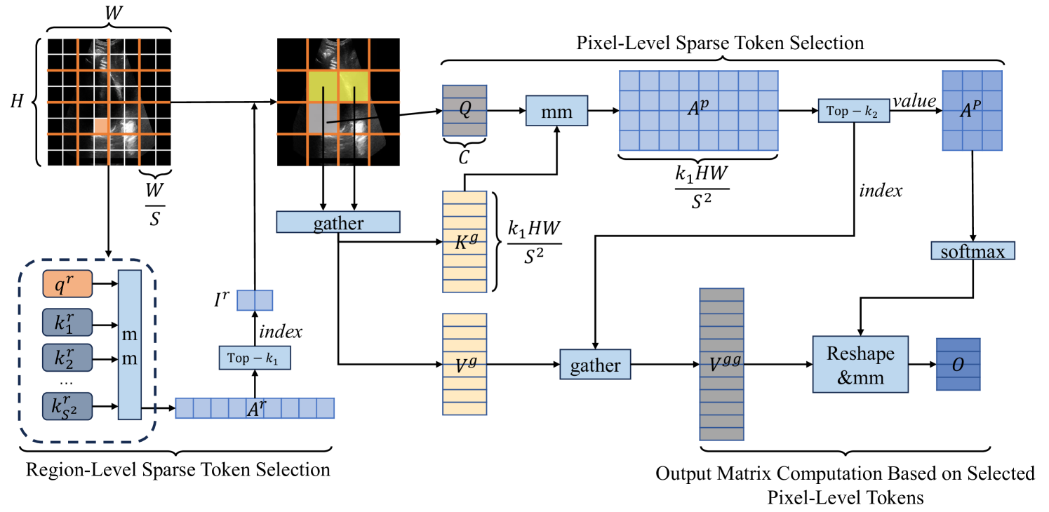
The core idea of DSSA is to explicitly perform sparse token selections at both region and pixel levels. It involves three main steps. First, for a given region-level token where the pixel-level token is located, mostly relevant regions are selected and irrelevant ones are filtered out according to the scores of attention matrix $\textbf{A}^{r}$ between region-level query $\mathbf{Q}^{r}$ and key $\mathbf{K}^{r}$. Second, for a given pixel-level token, mostly relevant pixels are selected, and irrelevant ones are filtered out by the scores of attention matrix $\textbf{A}^{p}$ between pixel-level query $\mathbf{Q}^{p}$ and key $\mathbf{K}^{p}$. Finally, the output matrix $O$ is computed by matrix multiplication between the normalized attention matrix $\textbf{A}^{p}$ and the pixel-level value $\mathbf{V}^{p}$. The conceptual diagram of DSSA is shown in Fig. 1. Following BiFormer [18], for a given input image $\mathbf{X}$ of size $H\times W\times C$, we divide the image into $S\times S$ non-overlapped regions, and obtain the region image $\mathbf{X^{r}}\in\mathbb{R}^{S^{2}\times\frac{HW}{S^{2}}\times C}$. Then, the region tokens: query, key, value, $\textbf{Q},\textbf{K},\textbf{V}\in\mathbb{R}^{S^{2}\times\frac{HW}{S^{2}}\times C}$, can be derived with linear projections:

where $S$ presents the number of regions, $r$ indicates that a token is region-level, ${\textbf{W}^{q}},{\textbf{W}^{k}},{\textbf{W}^{v}}\in{{\mathbb{R}}^{C\times C}}$ are corresponding projection weight matrices for the query, key, value, respectively.

As for the region-level sparse token selection, each region-level token query $\textbf{Q}^{r}\in\mathbb{R}^{S^{2}\times C}$ and key $\textbf{K}^{r}\in\mathbb{R}^{S^{2}\times C}$ can be derived by averaging all the pixel-level tokens on the region token $\mathbf{Q}$ and key $\mathbf{K}$. The attention map $\textbf{A}^{r}\in\mathbb{R}^{S^{2}\times S^{2}}$ between region-level queries $\mathbf{Q^{r}}$ and keys $\mathbf{K^{r}}$ is obtained through matrix multiplication, representing the semantic relevance between regions. Then, we employ a top-$k_{1}$ operation to select the $k_{1}$ most relevant regions for each region containing a given pixel-level token and record their indices in $\textbf{I}^{r}\in\mathbb{N}^{S^{2}\times k_{1}}$. The process is described as follows:

To fully leverage the GPU’s acceleration capabilities, the filtered region-level tokens need to be gathered back into a matrix.

where ${\textbf{K}^{g}},{\textbf{V}^{g}}\in{{\mathbb{R}}^{{S^{2}}\times{\frac{{k_{1}}HW}{S^{2}}}\times C}}$ are gathered key and value tensors, which will be further used to the pixel-level sparse token selection.

Concerning the pixel-level sparse token selection, for any pixel-level query in Q, we compute the relevance (i.e., attention matrix) between this query and the gathered pixel-level key in $\textbf{K}^{g}$, indicated as $\textbf{A}^{p}\in\mathbb{R}^{S^{2}\times\frac{HW}{S^{2}}\times\frac{k_{1}HW}{S^{2}}}$ as follows:

where $p$ means that this token is pixel-level. Additionally, since the first round of region-level sparse token selection involves an averaging operation within a region, which may retain noise features due to the overall high relevance. This could negatively impact the model’s ability to effectively extract features. Therefore, in $\textbf{A}^{p}$, we perform a second round of pixel-level sparse token selection using a top-$k_{2}$ operation, which not only selects the $k_{2}$ most relevant tokens but implicitly removes noises. The values and indices corresponding to the selected tokens are stored and denoted as $\textbf{A}^{P}\in\mathbb{R}^{S^{2}\times\frac{HW}{S^{2}}\times k_{2}}$ and $\textbf{I}^{P}\in\mathbb{N}^{S^{2}\times\frac{HW}{S^{2}}\times k_{2}}$, respectively:

where $k_{2}$ is determined by the scaling factor $\lambda$:

Similarly, to leverage GPU acceleration, $\textbf{V}^{g}$ is gathered based on $\textbf{I}^{P}$ to form $\textbf{V}^{gg}\in R^{S^{2}\times\frac{k_{1}HW}{S^{2}}\times k_{2}\times C}$:

Finally, $\textbf{V}^{gg}$ is weighted with $\textbf{A}^{P}$. Additionally, to preserve more fine-grained information beneficial for pixel-level segmentation, we add a local context enhancement term ($\mathrm{LCE}(\textbf{V})$) to the final output $\mathbf{O}$, which is a $5\times 5$ depth-wise convolution:

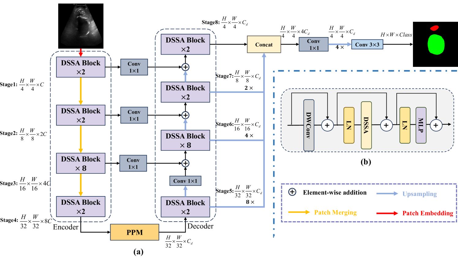
Based on this novel concept of DSSA attention, we can construct the core block of the model, the DSSA block, as shown in Fig. 2(b). Specifically, a $3\times 3$ depth-wise convolution is first used to encode relative positional information, followed by a layer normalization. DSSA is then applied to compute attention, followed by another a layer normalization, and the result is fed into a two-layer Multilayer Perceptron (MLP) module. During this process, three residual connections are employed to help alleviate the vanishing gradient and enhance the stability of the model. The DSSA block can be formulated as:

where $\mathbf{z}$ represents the output of each block, while $\hat{\mathbf{z}}$ indicates the output of the internal modules. $l$ denotes the $i$-th block.

DSSAU-Net is a hybrid CNN-Transformer architecture with the encoder-decoder structure built upon DSSA blocks, as shown in Fig. 2(a). As for Stage1, it consists of an overlapped patch embedding layer with two 3×3 convolutions and two DSSA blocks, which is used to transform the input image $\mathbf{X}$ of sizes $H\times W\times 3$ into the resulting feature map $\mathbf{X}_{1}$ of size $\frac{H}{4}\times\frac{W}{4}\times C$:

in Stage2, a Patch Merging layer is applied to reduce the number of tokens, and a linear embedding layer is used to increase the dimension $C$ to $2C$. Thus, the size of the feature map $\mathbf{X}_{2}$ output by Stage2, also containing two DSSA blocks, is $\frac{H}{8}\times\frac{W}{8}\times 2C$:

after that, similar process is repeated twice, the size of the corresponding feature maps $\mathbf{X}_{3}$ and $\mathbf{X}_{4}$ generated by Stage3 and Stage4 is $\frac{H}{16}\times\frac{W}{16}\times 4C$ and $\frac{H}{32}\times\frac{W}{32}\times 8C$, respectively, which are formulated as:

On the encoder side, the number of blocks in each stage is set to 2, 2, 8, and 2, respectively.

Since $\mathbf{X}_{4}$ aggregates contextual information from different stages, inspired by UperNet [15], we use the Pyramid Pooling Module (PPM) [17] to take full advantage of the rich semantic information contained in $\mathbf{X}_{4}$. On the decoder side, the dimension of the feature map is fixed to $C_{d}$. This setup helps reduce the number of parameters and ensures that features at different scales are equally important. Subsequently, the feature map of size $\frac{H}{32}\times\frac{W}{32}\times{C_{d}}$ is fed into the hierarchically built decoder from Stage5 to Stage8. During this process, the feature map in each stage is processed with DSSA attention and fused with the feature map of the same resolution from the encoder. The resulting feature map is then upsampled to the output size of $\frac{H}{4}\times\frac{W}{4}\times{C_{d}}$. The overall process can be described as:

where $\oplus$ presents element-wise addition.

Additionally, to effectively fuse the multiscale features in different stages, $\mathbf{X}_{5}$, $\mathbf{X}_{6}$, and $\mathbf{X}_{7}$ are upsampled to the same resolution as $\mathbf{X}_{8}$. All these upsampled feature maps are then concatenated along the channel dimension. After that, a $1\times 1$ convolution layer is applied, followed by $4\times$ upsampling, and another $3\times 3$ convolution layer. Finally, a feature map of resolution $H\times W\times Class$ is output to predict pixel-level segmentation. The process can be formulated as:

We adopt a hybrid loss function to train DSSAU-Net, combining dice loss ($\mathcal{L}_{dice}$) and cross-entropy loss ($\mathcal{L}_{ce}$). The dice loss helps alleviate class imbalance problems, while the cross-entropy loss ensures accurate pixel classification. These losses are defined as follows:

where $p_{i}$ is the predicted probability of the $i$-th pixel, and $g_{i}$ is the ground truth of the $i$-th pixel.

We conduct experiments on the competition dataset. The original dataset consists of 2,575 training images and 40 validation images. During training, all images are resized to $256\times 256$.

In this work, we employ three primary evaluation metrics to measure the segmentation performance of the model, namely the Dice Similarity Coefficient (DSC), the Hausdorff Distance (HD), and the Average Surface Distance (ASD). The specific calculations are presented as follows:

Additionally, to further demonstrate the effectiveness of our method in the ultrasound-assisted delivery process, during the final testing phase, we develop an automated program to calculate the Angle of Progression (AoP) and the Head-Symphysis Distance (HSD).

This work is conducted on a Geforce RTX 3090 GPU with 24GB of memory. We meticulously design the experimental details. Specifically, the input images are resized to a resolution of 256$\times$256, and the number of regions in each DSSA stage is set to 8$\times$8. In the encoder, the number of channels in each stage is set to [96, 192, 384, 768], and the $C_{d}$ of decoder is set to 64. Additionally, the initial learning rate is set to 1e-4. To improve the model’s generalization ability, we introduce several data augmentation strategies, such as rotation, flipping, and contrast adjustment. The backbone network uses weights pre-trained on the ImageNet dataset. The scaling factor $\lambda$ is set to 1/8.

We train our DSSAU-Net on the training set and evaluate the performance of DSSAU-Net on the validation set mentioned in Subsection 3.1. The evaluation is conducted using three segmentation metrics: DSC, HD, and ASD, as well as two key parameters related to ultrasound-assisted diagnosis: AoP and HSD. The results are presented in Table 1. It can be seen that DSSAU-Net achieves excellent segmentation results, with DSC, HD, and ASD reaching up to 86.43, 31.08, and 8.39, respectively, and has a low number of parameters and FLOPs. This reflects the effectiveness of both the designed U-shaped hierarchical network for the pubic symphysis and fetal head segmentation task and the DSSA mechanism in reducing computational resource consumption.

To further show the performance of DSSAU-Net, we compare it with the methods used by other teams in the MICCAI IUGC 2024 competition. The performance of classification and segmentation on the test set provided by the organizer, along with the final rank, is shown in Table 2. Our result wins fourth place in the classification and segmentation tasks in the competition. It can be seen that although DSSAU-Net did not achieve the highest final overall ranking, its performance on the segmentation task is still commendable. DSSAU-Net ranks second on both the HD and ASD metrics and third on the DSC metric, achieving an overall second place in the segmentation task. This demonstrates the strong capability of DSSAU-Net in handling segmentation tasks. However, its performance on the classification task is suboptimal, but this is in line with our expectations since our main goal is to develop a more accurate segmentation network. Overall, although DSSAU-Net performs well on the competition task and wins fourth place, it still has a large gap compared to the top-ranked team’s method. These gaps motivate us to continue our efforts to refine the network architecture and improve feature fusion strategies in future work.

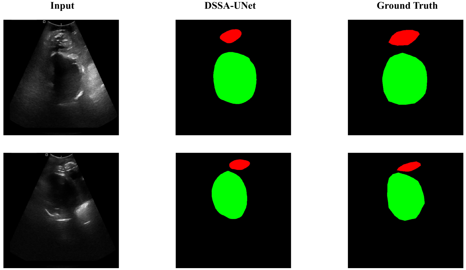
Additionally, we visualize the segmentation results and compare them with the ground truth, as shown in Fig. 3. One can see that the segmented masks generated by our approach closely match the boundaries and shape of ground truth.

In this section, to deeply explore the specific impact of each component of the DSSAU-Net on overall performance, we follow the above experimental settings and conduct a series of ablation studies on the provided training set and validation set. Specifically, we systematically analyze the effects of different factors, including the number of skip connections, the multiscale feature fusion module, and the selection of key hyperparameters in the proposed Dual Sparse Selection Attention.

References

- [1] Bellussi, F., Ghi, T., Youssef, A., Cataneo, I., Salsi, G., Simonazzi, G., Pilu, G.: Intrapartum ultrasound to differentiate flexion and deflexion in occipitoposterior rotation. Fetal Diagnosis and Therapy 42(4), 249–256 (2017)
- [2] Boyle, A., Reddy, U.M., Landy, H.J., Huang, C.C., Driggers, R.W., Laughon, S.K.: Primary cesarean delivery in the united states. Obstetrics & Gynecology 122(1), 33–40 (2013)
- [3] Cai, P., Lu, J., Li, Y., Lan, L.: Pubic symphysis-fetal head segmentation using pure transformer with bi-level routing attention (2023), https://arxiv.org/abs/2310.00289
- [4] Cao, H., Wang, Y., Chen, J., Jiang, D., Zhang, X., Tian, Q., Wang, M.: Swin-unet: Unet-like pure transformer for medical image segmentation. In: European conference on computer vision. pp. 205–218. Springer (2022)
- [5] Chen, Z., Lu, Y., Long, S., Campello, V.M., Bai, J., Lekadir, K.: Fetal head and pubic symphysis segmentation in intrapartum ultrasound image using a dual-path boundary-guided residual network. IEEE Journal of Biomedical and Health Informatics (2024)
- [6] Chen, Z., Ou, Z., Lu, Y., Bai, J.: Direction-guided and multi-scale feature screening for fetal head–pubic symphysis segmentation and angle of progression calculation. Expert Systems with Applications 245, 123096 (2024)
- [7] Cohen, S., Lipschuetz, M., Yagel, S.: Is a prolonged second stage of labor too long? Ultrasound in Obstetrics & Gynecology 50(4), 423–426 (2017)
- [8] Dupuis, O., Ruimark, S., Corinne, D., Simone, T., André, D., René-Charles, R.: Fetal head position during the second stage of labor: comparison of digital vaginal examination and transabdominal ultrasonographic examination. European Journal of Obstetrics & Gynecology and Reproductive Biology 123(2), 193–197 (2005)
- [9] Fiorentino, M.C., Villani, F.P., Di Cosmo, M., Frontoni, E., Moccia, S.: A review on deep-learning algorithms for fetal ultrasound-image analysis. Medical image analysis 83, 102629 (2023)
- [10] Ghi, T., Eggebø, T., Lees, C., Kalache, K., Rozenberg, P., Youssef, A., Salomon, L., Tutschek, B.: Isuog practice guidelines: intrapartum ultrasound. Ultrasound in Obstetrics & Gynecology 52(1), 128–139 (2018)
- [11] Malvasi, A., Tinelli, A., Barbera, A., Eggebø, T., Mynbaev, O., Bochicchio, M., Pacella, E., Di Renzo, G.: Occiput posterior position diagnosis: vaginal examination or intrapartum sonography? a clinical review. The Journal of Maternal-Fetal & Neonatal Medicine 27(5), 520–526 (2014)
- [12] Ramphul, M., Ooi, P.V., Burke, G., Kennelly, M.M., Said, S.A., Montgomery, A.A., Murphy, D.J.: Instrumental delivery and ultrasound: a multicentre randomised controlled trial of ultrasound assessment of the fetal head position versus standard care as an approach to prevent morbidity at instrumental delivery. BJOG: An International Journal of Obstetrics & Gynaecology 121(8), 1029–1038 (2014)
- [13] Ronneberger, O., Fischer, P., Brox, T.: U-net: Convolutional networks for biomedical image segmentation. In: Medical image computing and computer-assisted intervention–MICCAI 2015: 18th international conference, Munich, Germany, October 5-9, 2015, proceedings, part III 18. pp. 234–241. Springer (2015)
- [14] Rueda, S., Fathima, S., Knight, C.L., et al.: Evaluation and comparison of current fetal ultrasound image segmentation methods for biometric measurements: A grand challenge. IEEE Transactions on Medical Imaging 33(4), 797–813 (2014)
- [15] Xiao, T., Liu, Y., Zhou, B., Jiang, Y., Sun, J.: Unified perceptual parsing for scene understanding. In: Ferrari, V., Hebert, M., Sminchisescu, C., Weiss, Y. (eds.) Computer Vision – ECCV 2018. pp. 432–448. Springer International Publishing, Cham (2018)
- [16] Zhao, G., Lin, J., Zhang, Z., Ren, X., Su, Q., Sun, X.: Explicit sparse transformer: Concentrated attention through explicit selection (2019), https://arxiv.org/abs/1912.11637
- [17] Zhao, H., Shi, J., Qi, X., Wang, X., Jia, J.: Pyramid scene parsing network. In: Proceedings of the IEEE conference on computer vision and pattern recognition. pp. 2881–2890 (2017)
- [18] Zhu, L., Wang, X., Ke, Z., Zhang, W., Lau, R.: Biformer: Vision transformer with bi-level routing attention. In: 2023 IEEE/CVF Conference on Computer Vision and Pattern Recognition (CVPR). pp. 10323–10333 (2023)