DT-LSD: Deformable Transformer-based Line Segment Detection
Abstract
Line segment detection is a fundamental low-level task in computer vision, and improvements in this task can impact more advanced methods that depend on it. Most new methods developed for line segment detection are based on Convolutional Neural Networks (CNNs). Our paper seeks to address challenges that prevent the wider adoption of transformer-based methods for line segment detection. More specifically, we introduce a new model called Deformable Transformer-based Line Segment Detection (DT-LSD) that supports cross-scale interactions and can be trained quickly. This work proposes a novel Deformable Transformer-based Line Segment Detector (DT-LSD) that addresses LETR’s drawbacks. For faster training, we introduce Line Contrastive DeNoising (LCDN), a technique that stabilizes the one-to-one matching process and speeds up training by 34. We show that DT-LSD is faster and more accurate than its predecessor transformer-based model (LETR) and outperforms all CNN-based models in terms of accuracy. In the Wireframe dataset, DT-LSD achieves 71.7 for and 73.9 for ; while 33.2 for and 35.1 for in the YorkUrban dataset. Code available at: https://github.com/SebastianJanampa/DT-LSD.
1 Introduction
|
|
|
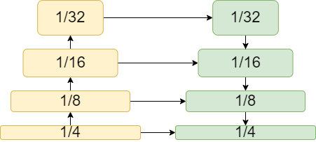
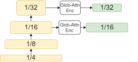
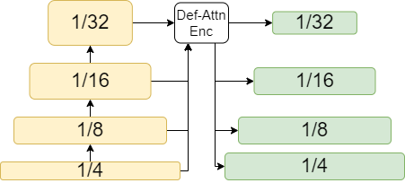
| a) Feature Pyramid Network | b) Global Attention Encoder | c) Deformable Attention Encoder |
Line segment detection is a low-level vision task used for higher-level tasks such as 3D reconstruction, camera calibration, vanishing point estimation, and scene understanding. Despite its importance, this problem remains open. Additionally, unlike other computer vision tasks (e.g. object detection, 3d-estimation, camera calibration), transformer-based models are not popular to tackle this challenge, LinE segment TRansformers (LETR) [21] is the only transformer model for line segment detection in the literature. Most recent methods [23, 28, 25, 27, 24] uses Convolutional Neural Networks (CNN) despite the fact that CNNs require a post-processing step to get the final predictions.
All models have a backbone that produces a set of hierarchical feature maps for further processing as shown in Fig. 1. CNN-based models use a feature pyramid network (FPN) as an enhancing method following the HourglassNet method [17] (see Fig. 1a). This method demonstrates the importance of cross-scale interaction since the new feature map is computed from contiguous feature maps, allowing the propagation of the global information from the highest-level feature map to the lower-level ones. On the other hand, LETR produces an enhanced feature map using a single feature map, as depicted in Fig. 1b. LETR demonstrates the ability of the global attention mechanism [18] to capture long-term relationships between the pixels of the same feature map (intra-scale processing), providing rich features.
This paper develops a new transformer-based models for line segment detection. First, we improve LETR’s feature map-enhancing method. We choose the deformable attention mechanism [29] for its ability to combine both intra- and cross-scale processing. We illustrate our idea in Fig. 1c, where a deformable-attention encoder is used for feature map enhancement. The encoder receives a set of hierarchical feature maps111feature maps are pre-processed by a to assure all the inputs have the same amount of channels. where for a pixel a fixed number of sampling offsets are generated for each given feature map. Second, we reduce the number of epochs required for training. Inspired from [10, 26], we propose Line Contrastive DeNoising (LCDN) as training technique to to accelerate the convergence of the training process. We show the efficiency of LCDN in Table 3 where we improve the metrics while keeping the same amount of epochs.
Our contributions are summarized as follows:
-
1.
We propose a novel end-to-end transformer-based framework showing that outperforms CNN-based line segment detectors. This is achieved by using the deformable attention mechanism.
-
2.
We introduce a highly-efficient training technique, Line Contrastive DeNoising, to reduce the number of epochs. This technique allows DT-LSD to achieve convergence in a similar number of epochs to CNN-based models.
- 3.
-
4.
Our work opens up opportunities for line segment detectors to remove hand-crafted post-processing by utilizing end-to-end transformer-based models.
In what remains of this paper, we describe previous state-of-the-art methods in line segment detection, as well as the two attention mechanisms in Sec. 2. Next, we describe the methodology for DT-LSD in Sec. 3. Then, we provide information about model parameters and training settings, comparison against previous state-of-the-art models, and the ablation studies of DT-LSD in Sec. 4. Finally, we summarize our findings in Sec. 5.
2 Background
2.1 Line Segment Detection
2.1.1 Traditional Approaches
The Hough Transform (HT) [7] remains an important method for line detection. First, the Hough Transform applies Canny edge detection [1] to obtain line segment candidates. Candidate lines are represented in polar form. Here, we note that candidate lines are evaluated based on the overlapping number of pixels between the lines and the detected edges. Variations include the use of the Radon Transform and the Revoting Hough Transform.
In regions dominated by a large density of edges, the HT can generate a large number of false positives. Grompone von Gioi et al. proposed a linear-time Line Segment Detector (LSD) [19] to address this problem. LSD uses line-supported regions and line segment validation. The approach also reduced time complexity through the use of a pseudo-sorting algorithm based on gradient magnitudes. A fundamental advantage of traditional methods is that they do not require training for specific datasets.
2.1.2 Deep Learning Based Approaches
Learning-based line segment detectors have shown significant improvements compared to traditional approaches. The methods include different approaches that focus on line junctions, attraction field maps (AFM), transformers, and combining traditional approaches with deep learning techniques.
The Holistically-Attracted Wireframe Parser (HAWP) [23] proposed a 4-dimensional attraction field map, and later HAWPv2 [24], a hybrid model of HAWP and self-supervision, was introduced. MLNet [25] and SACWP [27] incorporated cross-scale feature interaction on HAWP model. In [22, 28], the authors developed a method for detecting line junctions which were used to provide candidate line segments. Then, a classifier validated the candidates and produced the final set of predicted line segments. LSDNet [18] used a CNN model to generate an angle field and line mask that were used to detect line segments using the LSD method. HT-HAWP and HT-LCNN [14] added global geometric line priors through the Hough Transform in deep learning networks to address the lack of labeled data. However, the above methods requires of post-processing steps to produce the final output. In contrast, Line segment transformers (LETR) [21] remove post-processing steps by using an end-to-end transformer-based model that relies on a coarse-to-fine strategy with two encoder-decoder transformer blocks.
2.2 Transformers
2.2.1 High-complexity of Global Attention Models
One crucial factor of LETR’s slow convergence is the global attention mechanism, which only does intra-scale feature processing. Plus, the global attention leads to very high computational complexity.
To understand the complexity requirements of LETR, we revisit the global attention mechanism. We define global attention using [18]:
| (1) |
where represent the queries, keys, values and the hidden dimensions, respectively. For object and line segment detection, we define as the flattened form of the feature map where and are the height and width, respectively. In the encoder, we have resulting in a complexity time of . Similarly, for the decoder, we have where is the number of queries producing a complexity time of .
2.2.2 Deformable Attention Module
Based on our previous discussion, it is clear that the bottleneck of transformer-based models is the encoder, whose complexity time quadratically increases with respect to the spatial size of the feature map. To address this issue, Zhu et al. [29] proposed the deformable attention mechanism, inspired by deformable convolution [3]. Unlike global attention, the deformable attention module only attends to a fixed number of keys for each query (see Fig. 2 from [29] for a visual representation).
Given an input feature map , let be the index of a query element with content feature and a 2d-reference point , the deformable attention for one attention head222The multi-head deformable attention equation is in page 5 section 4.1 in [29] is mathematically defined as
| (2) |
where indexes the sampling keys and is the total sampling keys number (). The sampling key is computed as where is the sampling offset. is the row of the attention weight . The weights of satisfy .
Comparing Eq. 1 to Eq. 2, is replaced by , and by . So, the complexity time for the deformable encoder is , which has a linear complexity. For the deformable decoder, the complexity time is where is the total number of queries, and the spatial dimensions of are irrelevant.
Apart from reducing the memory and time complexities, deformable attention has a variation called multi-scale deformable attention () that allows cross-scale feature interaction and is defined as
| (3) |
where is a set of multi-scale feature maps, and . The normalized 2d coordinates has its values lying in the range of , and is re-scaled to dimensions of the -level feature map by the function . Like Eq. 2, the attention weight satisfies .
3 Methodology
3.1 Overview
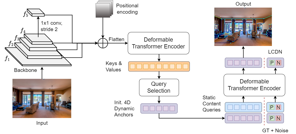
We present the architecture of DT-LSD, an end-to-end deformable transformer for line segment detection, in Fig. 2. First, we pass an RGB image to a backbone to produce a set of hierarchical feature maps. Second, a deformable encoder enhances the backbone’s feature maps. Third, we apply query selection to choose the top-K queries 333In the encoder, feature maps pixels are treated as queries as the initial 4D dynamic line endpoints. Fourth, we feed the initial dynamic line endpoints and the static (learnable) content queries to the deformable decoder to promote the interaction between queries and the enhanced feature maps. Fifth, two independent multi-layer perceptron networks process the decoder’s output queries to estimate the line segment endpoints and classify whether a query contains a line. For the training process, we added an extra branch to perform line contrastive denoising, which did not affect the inference time. In this section, we do not describe the decoder and the one-to-one matching since they are already described in [29] and [21].
3.2 Deformable Transformer Encoder
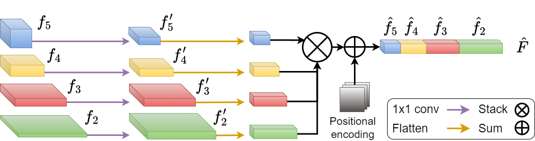
The encoder is a fundamental part of our network since it enhances the backbone’s feature maps. However, these feature maps do not have any dimensions in common. For this reason, it is important to pre-process them before passing them to the encoder. As shown in Fig. 3, given an RGB image of dimensions , the backbone produces a set of hierarchical feature maps where and and . Since do not have any dimension in common and we do not want to lose spatial resolution, we apply a convolution to each feature so that the whole set has the same number of channels where . Next, we flatten their spatial dimension, followed by stacking them together and adding the position encoding (), creating the vector
| (4) |
where and 444The and functions are associative functions., .
We pass to the encoder where each of its stacked pixels is treated as a query . For each query, we produce a fixed number of offsets per feature map followed by applying Eq. 3. In general, we compute a total of 16 offsets per attention head, where 4 of them are for intra-scale interaction, and the other 12 are for cross-scale interaction. Besides combining both types of interactions, we address the global attention’s time complexity and the convolutional layers’ kernel space restriction.
3.3 Line Contrastive Denoising Technique
A problem for end-to-end transformer-based methods is the one-to-one matching technique, which removes the need for non-maximum suppression (NMS) but is unstable in matching queries with ground truth. The main difference between one-to-one matching and NMS is that the first one uses scores to do the matching. In contrast, the second one eliminates candidates depending on how much the bounding boxes of the candidates belonging to the same class overlap.
In this section, we present Line Contrastive Denoising (LCDN), a training technique for stabilizing the matching process inspired from [26]. While LCDN is used to speed up training, it is not part of the final inference model. LCDN facilitates the matching by teaching the Hungarian Matcher to accept queries whose predicted line’s endpoints lie on or are close to a ground-truth line and to reject queries whose predicted line’s endpoints are far away from the ground-truth line. To achieve this, we create positive and negative queries by performing line length scaling and line rotation. The length scaling consists of varying the length of the line segment, with original length , such that positive queries have a length in a range of and the negative queries . For line rotation, we rotate the line in a range of for positive, where is the fixed angle. For negative queries, the rotation is in the range. We present an example of our LCDN technique in Fig. 4b and a comparison against the Contrastive DeNoising (CDN) [26] in Table 3.
Since LCDN generates extra groups of denoising queries from ground-truth lines, this can harm the training process if the prediction queries interact with the denoising queries. The denoising queries contain ground-truth information, so if a matching query sees this information, it will start training with information that should not be known. In the other case, we want the denoising queries to see the information stored by the matching queries. We manually implement this by using an attention mask. Note that only queries from the same denoising group are allowed to interact with each other, but all denoising groups interact with the matching group.
 |
 |
| a) CDN (DINO) | b) LCDN (ours) |
| Ground Truth | Positive query | Negative query |
3.4 Loss Function
We choose the focal loss [12] for line classification because it can deal with class imbalance. The focal loss encourages training on uncertain samples by penalizing samples with predicted probability that is away from 0 or 1 as given by (per sample loss):
| (5) |
with , , and .
For each line candidate , we use the loss to compute the distance from the ground truth points. Let denote the line candidate. If the classifier accepts the line candidate, we get for the classification output. Else, . Let denote the endpoint component of the -th ground-trtuh line. We have four endpoint components because we use two coordinate points representing the line segment. The loss function is then given by:
| (6) |
where is the indicator function based on the classifier output .
The final loss is a linear combination of the two loss functions:
| (7) |
where , , and is the total number of instances.
| Parameter | Value |
|---|---|
| number of feature maps | 4 |
| number of encoder layers | 6 |
| encoder sampling points | 4 |
| number of decoder layers | 6 |
| decoder sampling points | 4 |
| hidden dim | 256 |
| feedforward dim | 1024 |
| number of heads | 8 |
| number of classes | 2 |
| number of queries | 900 |
| denoising number | 300 |
| label noise ratio | 0.5 |
| line scaling | 1.0 |
| line rotation | 7∘ |
| line loss weight | 5 |
| class loss weight | 2 |
| optimizer | AdamW |
| initial learning rate | 1e-4 |
| initial learning rate of backbone | 1e-5 |
| weight decay | 1e-4 |
| batch size | 2 |
| total number of epochs | 24 |
| learning rate drop | 21 |
4 Results
4.1 Datasets
ShangaiTech Wireframe Dataset. We used the ShangaiTech Wireframe dataset for comparisons [9]. The dataset consists of 5462 (indoor and outdoor) images of hand-made environments. The ground-truth line segments were manually labeled. The goal of the dataset was to provide line segments with meaningful geometric information about the scene. We split the dataset into 5000 images for training and 462 for testing.
York Urban Dataset. We also use the York Urban dataset [6]. The dataset consists of 122 (45 indoor and 57 outdoor) images of size pixels. Denis et al. generated ground-truth line segments using an interactive MATLAB program with a sub-pixel precision. We only used this dataset for testing.
For the results shown in Sec. 4.3, we follow [15, 2, 29, 26, 10] and apply data augmentations to the training set. During training, we reprise the input images such that the shortest side is at least 480 and at most 800 pixels while the longest at most 1333. At the evaluation stage, we resize the image with the shortest side at least 640 pixels.
| Method | Epochs | Wireframe Dataset | YorkUrban Dataset | FPS | ||||||||||||||
| sAP10 | sAP15 | sF10 | sF15 | AP | F | sAP10 | sAP15 | sF10 | sF15 | AP | F | |||||||
| Traditional methods | ||||||||||||||||||
| LSD [19] | / | / | / | / | / | 55.2 | 62.5 | / | / | / | / | 50.9 | 60.1 | 49.6 | ||||
| CNN-based methods | ||||||||||||||||||
| DWP [9] | 120 | 5.1 | 5.9 | / | / | 67.8 | 72.2 | 2.1 | 2.6 | / | / | 51.0 | 61.6 | 2.24 | ||||
| AFM [22] | 200 | 24.4 | 27.5 | / | / | 69.2 | 77.2 | 9.4 | 11.1 | / | / | 48.2 | 63.3 | 13.5 | ||||
| L-CNN [28] | 16 | 62.9 | 64.9 | 61.3 | 62.4 | 82.8 | 81.3 | 26.4 | 27.5 | 36.9 | 37.8 | 59.6 | 65.3 | 10.3 | ||||
| HAWP [23] | 30 | 66.5 | 68.2 | 64.9 | 65.9 | 86.1 | 83.1 | 28.5 | 29.7 | 39.7 | 40.5 | 61.2 | 66.3 | 30.3 | ||||
| F-Clip [4] | 300 | 66.8 | 68.7 | / | / | 85.1 | 80.9 | 29.9 | 31.3 | / | / | 62.3 | 64.5 | 28.3 | ||||
| ULSD [11] | 30 | 68.8 | 70.4 | / | / | / | / | 28.8 | 30.6 | / | / | / | / | 36.8 | ||||
| HAWPv2 [24] | 30 | 68.6 | 70.2 | / | / | 81.5 | 29.1 | 30.4 | / | / | 61.6 | 64.4 | 14.0 | |||||
| SACWP [27] | 30 | / | / | / | / | 30.0 | 31.8 | / | / | / | / | 34.8 | ||||||
| MLNET [25] | 30 | / | / | 81.4 | / | / | 65.1 | 12.6 | ||||||||||
| Transformer-based methods | ||||||||||||||||||
| LETR [21] | 825 | 65.2 | 67.7 | 86.3 | 29.4 | 31.7 | 62.7 | 5.8 | ||||||||||
| DT-LSD (ours) | 24 | 71.7 | 73.9 | 70.1 | 71.2 | 89.1 | 85.8 | 33.2 | 35.1 | 44.5 | 45.8 | 65.9 | 68.0 | 8.9 | ||||
4.2 Implementation
4.2.1 Network
We use the SwinL [16] as a backbone for our deformable encoder-decoder transformer model. For the deformable transformer, we followed the recommendation of DINO [26]. We used 4 sampling offsets for the encoder and decoder, 900 queries to predict line segments, 6 stacked-encoder layers, and 6 stacked-decoder layers. We summarize the DT-LSD architecture parameters and training parameters in Table 1. We train DT-LSD on a single Nvidia RTX A5500 GPU with a batch size of 2.
4.3 Comparison to SOTA models
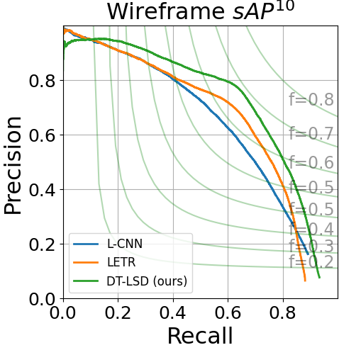
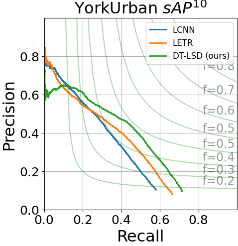
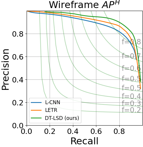
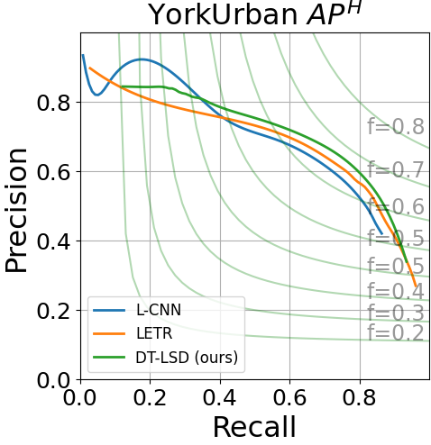
We compare DT-LSD to many state-of-the-art models in Table 2. Our approach gives the most accurate result in all of our comparisons providing new state-of-the-art results in both datasets. In the Wireframe dataset, DT-LSD performs better than SCAWP (the second best result) by around 2 points in the sAP metric. In the YorkUrban dataset, DT-LSD outperforms MLNET (the second best result) by around 1 percentage point in the sAP metric and 1.6 in the AP. Comparing to LETR, we show a significant gain in all metrics. Furthermore, we note that DT-LSD is trained with just 24 epochs, significantly faster than the 825 epochs required for LETR. At the same time, DT-LSD runs at nearly 9 frames per second.
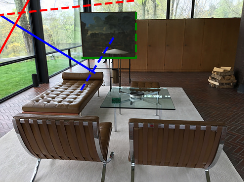
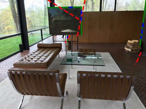
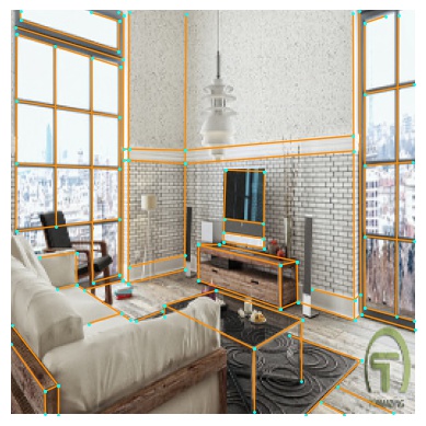
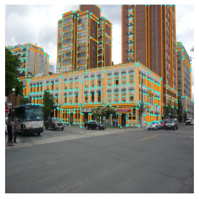
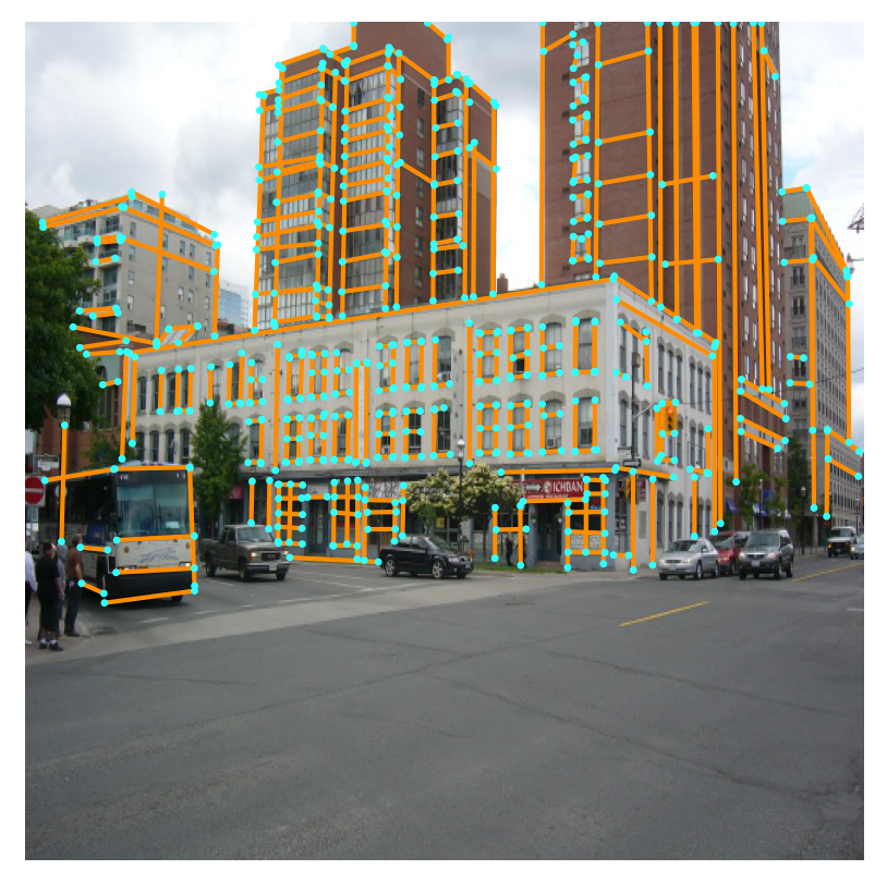
We show the Precision-Recall (PR) curves for sAP10 and AP in Fig. 5. DT-LSD has low performance for low recall values but surpasses LETR and L-CNN for recall values greater than 0.1. We also provide qualitative comparative results in Fig. 6. The images clearly show that the transformer-based approaches (LETR and DT-LSD) perform significantly better than LCNN and HAWP. Upon closer inspection, we can see that DT-LSD avoids noisy line detections that appear in LETR (e.g., inspect the center regions of third-row images).
4.4 Ablation Studies
4.4.1 Line Contrastive Denoising
Our comparisons are based on the number of epochs and the sAP metric as summarized in Table 3. For a fair comparison, we train all the DINO555We use DINO-ResNet50-4scale from [26]. variations using ResNet50 [8] as the backbone.
Compared to the 500 epochs required for the vanilla DETR, DINO converges at just 36 epochs. Furthermore, plain DINO results in a maximum accuracy drop of 0.6, while our additions boost performance significantly (e.g., compare 66.3 and 68.8 versus 53.8 and 57.2).
The performance improvement against vanilla DETR is because DINO uses the MultiScale Deformable Attention mechanism described in Eq. 3, which promotes the cross- and intra-scale interaction. However, DINO has a lower performance than LETR. Fig. 4 shows that the contrastive denoising (CDN) technique from DINO does not work for line segments because applying CDN to line segments results in scaling and translating both positive and negative queries. Therefore, these two operations lead to the model accepting non-line-segment candidates as potential candidates. We test our idea by removing the box scaling. We noticed an improvement of around 7 points for sAP10. We gain 3 extra points for sAP10 by adding the line scaling technique, reaching a score of . By combining the line scaling and the line rotation (our line contrastive denoising technique), we obtain the maximum of in sAP10.
Based on our experiments, we conclude that our enhancing method and training technique are effective since DINO with LCDN outperforms LETR using a lower-parameter backbone and fewer training epochs. We want to highlight that the input size of the image for all DINO variations was for both training and testing. On the other hand, vanilla DETR and LETR resize the images following the procedure described in Sec. 4.1 for training, and they resize the image with the shortest side of at least 1100 pixels for testing.
| Model | Epochs | sAP5 | sAP10 | sAP15 |
|---|---|---|---|---|
| Vanilla DETR | 500 | - | 53.8 | 57.2 |
| LETR | 825 | - | 65.2 | 67.1 |
| DINO | 36 | 45.8 | 53.2 | 56.7 |
| - box scaling | 36 | 51.7 | 60.0 | 63.5 |
| + line scaling | 36 | 56.5 | 63.4 | 66.2 |
| + line rotation | 36 | 60.7 | 66.3 | 68.7 |
4.4.2 Feature maps
An important element of our model is the feature maps generated by the backbone. Here, we evaluate the effectiveness of different feature maps and backbones. We report the results in Table 4. All models are trained using 24 epochs. Adding the S1 feature map produces more precise line segments while slowing down our inference time (measured in the number of frames per second (FPS)). Using SwinL as the backbone gives the best results, but slows down the inference speed. For example, the configuration SwinL with 5 feature maps achieves a score of in the sAP10 at 10.5 FPS.
4.4.3 Image upsampling
Most transformer-based algorithms use upsampling techniques to improve their performance. To evaluate the effects of upsampling an image, we train and test our model at different resolutions for 24 epochs. As documented in Table 5, upsampling benefits both CNN- and transformer-based models. First, we train DT-LSD following popular CNN-based methods by resizing the original image to 512512. For DT-LSD 512, we obtain the fastest inference time at 13.6 FPS among all DT-LSD variations.
Motivated by DETR-based models [2, 29, 15, 10, 21, 26, 20], we also apply scale augmentation consisting of resizing the input image so that the shortest side is a minimum of 480 pixels and a maximum of 800 pixels, while the longest side is a maximum of 1333 pixels. Here, we choose five different testing sizes, 1) 480, the minimum size used for training, 2), 512, the size used for CNN-based line segment detectors, 3) 640, the size use for YOLO detectors, 4) 800, the maximum size used for training, and 5) 1100, LETR’s [21] testing size.
We note that this scaling technique improved our results over 512512. For example, DT-LSD 480† produces better results than DT-LSD 512. As the testing size increases, the sAP metric improves while reducing inference speed (as measured by FPS). As a balance between speed and precision, we choose DT-LSD 640† because it increases sAP10 and sAP15 by around 2 points, while its FPS is only by 2.9 fps less than DT-LSD 520†. We did not choose DT-LSD 800† because the 0.4 improvement in sAP does not justify a drop of 2.5 fps in inference performance.
| Model | Train | Test | sAP10 | sAP15 | FPS |
|---|---|---|---|---|---|
| Size | Size | ||||
| HAWP | 512 | 512 | 65.7 | 67.4 | - |
| HAWP | 832 | 832 | 67.7 | 69.1 | - |
| HAWP | 832 | 1088 | 65.7 | 67.1 | - |
| DT-LSD | 512 | 512 | 67.8 | 70.3 | 13.6 |
| DT-LSD | 800∗ | 480† | 69.0 | 71.5 | 12.2 |
| DT-LSD | 800∗ | 520† | 69.5 | 71.8 | 11.8 |
| DT-LSD | 800∗ | 640† | 71.7 | 73.9 | 8.9 |
| DT-LSD | 800∗ | 800† | 72.3 | 74.3 | 6.4 |
| DT-LSD | 800∗ | 1100† | 72.2 | 74.2 | 4.7 |
4.4.4 Training Epochs
We report the results for training DT-LSD with 12, 24, and 36 epochs in Table 6. DT-LSD gets to competitive performance after training with just 12 epochs. At 12 epochs, DT-LSD achieves a sAP10 of 68.4. There is very little difference between 24 and 36 epochs. At 36 epochs, we get a minor increase of 0.3, 0.2, and 0.1 in the sAP5, sAP10, and sAP15, respectively.
| Number of Epochs | sAP5 | sAP10 | sAP15 |
|---|---|---|---|
| 12 | 65.2 | 68.4 | 69.7 |
| 24 | 66.6 | 71.7 | 73.9 |
| 36 | 66.9 | 71.9 | 74.0 |
4.4.5 Transfer Learning
We report results based on pre-training on different datasets in Table 7. For our experiments, we use 24 epochs. In our first example, the backbone was pre-trained with the ImageNet-22k dataset [5]. In our second example, the DINO was pre-trained using the COCO object detection dataset [13]. From the results, it is clear that it is essential to pre-train the entire network and not just the backbone.
| Pretrained Weights | sAP5 | sAP10 | sAP15 |
|---|---|---|---|
| ImageNet-22k | 10.8 | 12.7 | 15.6 |
| COCO | 66.6 | 71.7 | 73.9 |
5 Conclusion
We introduced DT-LSD, a transformer-based model for line segment detection. DT-LSD uses cross-scale interactions to speed up convergence and improve results. Our approach uses pre-training on the COCO dataset to learn low-level features. Our extensive experiment showed that end-to-end transformer-based model can surpass CNN-based methods. Additionally, we opened new opportunities for new line segment detection methods that do not require post-processing steps.
In future work, we will consider the development of specialized backbones for transformer-based models. Additionally, an important observation from this work is that DT-LSD needs the COCO pre-trained weights to achieve state-of-the-art results. Therefore, we will also focus on the implementation of the network that is trained from scratch.
References
- [1] John Canny. A computational approach to edge detection. IEEE Transactions on Pattern Analysis and Machine Intelligence, PAMI-8(6):679–698, 1986.
- [2] Nicolas Carion, Francisco Massa, Gabriel Synnaeve, Nicolas Usunier, Alexander Kirillov, and Sergey Zagoruyko. End-to-end object detection with transformers. In European conference on computer vision, pages 213–229. Springer, 2020.
- [3] Jifeng Dai, Haozhi Qi, Yuwen Xiong, Yi Li, Guodong Zhang, Han Hu, and Yichen Wei. Deformable convolutional networks. In Proceedings of the IEEE international conference on computer vision, pages 764–773, 2017.
- [4] Xili Dai, Haigang Gong, Shuai Wu, Xiaojun Yuan, and Yi Ma. Fully convolutional line parsing. Neurocomputing, 506:1–11, 2022.
- [5] Jia Deng, Wei Dong, Richard Socher, Li-Jia Li, Kai Li, and Li Fei-Fei. Imagenet: A large-scale hierarchical image database. In 2009 IEEE conference on computer vision and pattern recognition, pages 248–255. IEEE, 2009.
- [6] Patrick Denis, James H Elder, and Francisco J Estrada. Efficient edge-based methods for estimating manhattan frames in urban imagery. In Computer Vision–ECCV 2008: 10th European Conference on Computer Vision, Marseille, France, October 12-18, 2008, Proceedings, Part II 10, pages 197–210. Springer, 2008.
- [7] Richard O. Duda and Peter E. Hart. Use of the hough transformation to detect lines and curves in pictures. Commun. ACM, 15(1):11–15, jan 1972.
- [8] Kaiming He, Xiangyu Zhang, Shaoqing Ren, and Jian Sun. Deep residual learning for image recognition. In Proceedings of the IEEE conference on computer vision and pattern recognition, pages 770–778, 2016.
- [9] Kun Huang, Yifan Wang, Zihan Zhou, Tianjiao Ding, Shenghua Gao, and Yi Ma. Learning to parse wireframes in images of man-made environments. In CVPR, June 2018.
- [10] Feng Li, Hao Zhang, Shilong Liu, Jian Guo, Lionel M Ni, and Lei Zhang. Dn-detr: Accelerate detr training by introducing query denoising. In Proceedings of the IEEE/CVF Conference on Computer Vision and Pattern Recognition, pages 13619–13627, 2022.
- [11] Hao Li, Huai Yu, Jinwang Wang, Wen Yang, Lei Yu, and Sebastian Scherer. Ulsd: Unified line segment detection across pinhole, fisheye, and spherical cameras. ISPRS Journal of Photogrammetry and Remote Sensing, 178:187–202, 2021.
- [12] Tsung-Yi Lin, Priya Goyal, Ross Girshick, Kaiming He, and Piotr Dollár. Focal loss for dense object detection. In Proceedings of the IEEE international conference on computer vision, pages 2980–2988, 2017.
- [13] Tsung-Yi Lin, Michael Maire, Serge Belongie, James Hays, Pietro Perona, Deva Ramanan, Piotr Dollár, and C Lawrence Zitnick. Microsoft coco: Common objects in context. In Computer Vision–ECCV 2014: 13th European Conference, Zurich, Switzerland, September 6-12, 2014, Proceedings, Part V 13, pages 740–755. Springer, 2014.
- [14] Yancong Lin, Silvia L Pintea, and Jan C van Gemert. Deep hough-transform line priors. 2020.
- [15] Shilong Liu, Feng Li, Hao Zhang, Xiao Yang, Xianbiao Qi, Hang Su, Jun Zhu, and Lei Zhang. DAB-DETR: Dynamic anchor boxes are better queries for DETR. In International Conference on Learning Representations, 2022.
- [16] Ze Liu, Yutong Lin, Yue Cao, Han Hu, Yixuan Wei, Zheng Zhang, Stephen Lin, and Baining Guo. Swin transformer: Hierarchical vision transformer using shifted windows. In Proceedings of the IEEE/CVF International Conference on Computer Vision (ICCV), 2021.
- [17] Alejandro Newell, Kaiyu Yang, and Jia Deng. Stacked hourglass networks for human pose estimation. In Bastian Leibe, Jiri Matas, Nicu Sebe, and Max Welling, editors, Computer Vision - 14th European Conference, ECCV 2016, Proceedings, Lecture Notes in Computer Science (including subseries Lecture Notes in Artificial Intelligence and Lecture Notes in Bioinformatics), pages 483–499, Germany, 2016. Springer Verlag. Publisher Copyright: © Springer International Publishing AG 2016.; 14th European Conference on Computer Vision, ECCV 2016 ; Conference date: 08-10-2016 Through 16-10-2016.
- [18] Ashish Vaswani, Noam Shazeer, Niki Parmar, Jakob Uszkoreit, Llion Jones, Aidan N Gomez, Ł ukasz Kaiser, and Illia Polosukhin. Attention is all you need. In I. Guyon, U. Von Luxburg, S. Bengio, H. Wallach, R. Fergus, S. Vishwanathan, and R. Garnett, editors, Advances in Neural Information Processing Systems, volume 30. Curran Associates, Inc., 2017.
- [19] R.G. von Gioi, J. Jakubowicz, J.-M. Morel, and G. Randall. LSD: A fast line segment detector with a false detection control. IEEE Transactions on Pattern Analysis and Machine Intelligence, 32(4):722–732, apr 2010.
- [20] Yingming Wang, Xiangyu Zhang, Tong Yang, and Jian Sun. Anchor detr: Query design for transformer-based detector. In Proceedings of the AAAI Conference on Artificial Intelligence, volume 36, pages 2567–2575, 2022.
- [21] Yifan Xu, Weijian Xu, David Cheung, and Zhuowen Tu. Line segment detection using transformers without edges. In Proceedings of the IEEE/CVF Conference on Computer Vision and Pattern Recognition, pages 4257–4266, 2021.
- [22] Nan Xue, Song Bai, Fudong Wang, Gui-Song Xia, Tianfu Wu, and Liangpei Zhang. Learning attraction field representation for robust line segment detection. In IEEE Conference on Computer Vision and Pattern Recognition (CVPR), 2019.
- [23] Nan Xue, Tianfu Wu, Song Bai, Fu-Dong Wang, Gui-Song Xia, Liangpei Zhang, and Philip H.S. Torr. Holistically-attracted wireframe parsing. In CVPR, 2020.
- [24] Nan Xue, Tianfu Wu, Song Bai, Fu-Dong Wang, Gui-Song Xia, Liangpei Zhang, and Philip HS Torr. Holistically-attracted wireframe parsing: From supervised to self-supervised learning. IEEE Transactions on Pattern Analysis and Machine Intelligence, 2023.
- [25] Jian Yang, Yuan Rao, Qing Cai, Eric Rigall, Hao Fan, Junyu Dong, and Hui Yu. Mlnet: An multi-scale line detector and descriptor network for 3d reconstruction. Knowledge-Based Systems, 289:111476, 2024.
- [26] Hao Zhang, Feng Li, Shilong Liu, Lei Zhang, Hang Su, Jun Zhu, Lionel M. Ni, and Heung-Yeung Shum. Dino: Detr with improved denoising anchor boxes for end-to-end object detection, 2022.
- [27] Jiahui Zhang, Jinfu Yang, Fuji Fu, and Jiaqi Ma. Structural asymmetric convolution for wireframe parsing. Engineering Applications of Artificial Intelligence, 128:107410, 2024.
- [28] Yichao Zhou, Haozhi Qi, and Yi Ma. End-to-end wireframe parsing. In ICCV 2019, 2019.
- [29] Xizhou Zhu, Weijie Su, Lewei Lu, Bin Li, Xiaogang Wang, and Jifeng Dai. Deformable detr: Deformable transformers for end-to-end object detection. arXiv preprint arXiv:2010.04159, 2020.