Duality for pairs of upward bipolar plane graphs and submodule lattices
Abstract.
Let and be acyclic, upward bipolarly oriented plane graphs with the same number of edges. While can symbolize a flow network, has only a controlling role. Let and be bijections from , …, to the edge set of and that of , respectively; their role is to define, for each edge of , the corresponding edge of . Let be an element of an Abelian group . An -tuple , , of elements of is a solution of the paired-bipolar-graphs problem , , if whenever is the “all-or-nothing-flow” capacity of the edge for , …, and is a maximal directed path of , then by fully exploiting the capacities of the edges corresponding to the edges of and neglecting the rest of the edges of , we have a flow process transporting from the source (vertex) of to the sink of . Let , , , where and are the “two-outer-facet” duals of and , respectively, and and are defined naturally. We prove that and have the same solutions. This result implies George Hutchinson’s self-duality theorem on submodule lattices.
Key words and phrases:
Upward plane graph, edge capacity, George Hutchinson’s self-duality theorem, lattice identity1991 Mathematics Subject Classification:
06C05, 05C211. Introduction
We present and prove the main result in Sections 2—4, intended to be readable for most mathematicians. Section 5, an application of the preceding sections, presupposes a modest familiarity with some fundamental concepts from (universal) algebra and, mainly, from lattice theory.
Sections 2–4 prove a duality theorem, Theorem 1, for some pairs of finite, oriented planar graphs. The first graph, , is a flow network with edge capacities belonging to a fixed Abelian group. The other graph plays a controlling role: each of its maximal paths determines a set of edges of to be used at their full capacities while neglecting the rest of the edges; see Section 2 for a preliminary illustration.
2. An introductory example
Before delving into the technicalities of Section 3, consider the following example.
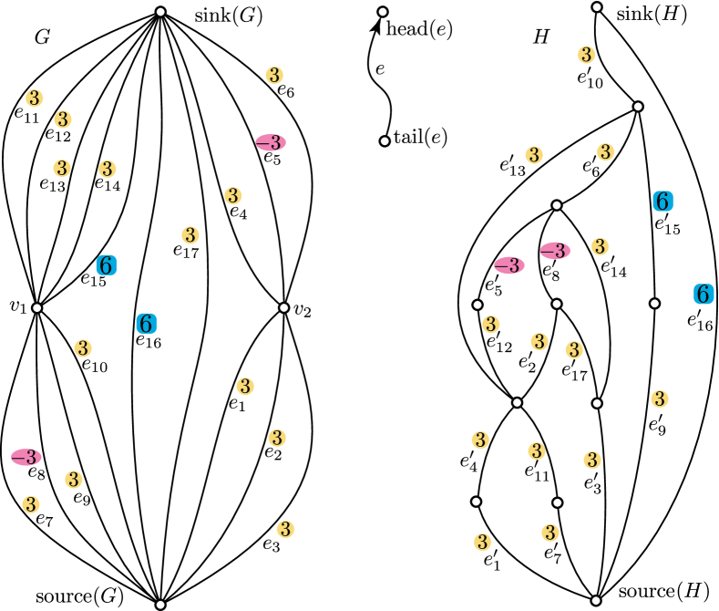
In Figure 1, and are oriented graphs. With the convention that every edge is upward oriented (like in the case of Hasse diagrams of partially ordered sets), the arrowheads are omitted. The subscripts supply a bijective correspondence between the edge set of and that of . We can think of as a hypothetical concrete system in which the arcs (i.e., the edges) are transit routes, pipelines, fiber-optic cables, or freighters (or passenger vehicles) traveling on fixed routes, etc. The numbers in colored geometric shapes are the capacities of the arcs of . (Even though we repeat these numbers on the arcs of , they still mean the capacities of the corresponding arcs of ; the arcs of have no capacities.) These numbers are “all-or-nothing-flow” capacities, that is, each arc should be either used at full capacity or avoided; this stipulation is due to physical limitations or economic inefficiency. (However, there can be parallel arcs with different capacities; see, for example, and .) The vertices of are repositories (or warehouses, depots, etc.). In contrast to , the graph is to provide visual or digital information within a hypothetical control room. Each maximal directed path of defines a method to transport exactly units (such as pieces, tons, barrels, etc.) of something from to without changing the final contents of other repositories. For example, , , is a maximal directed path of ; its meaning for is that we use exactly the arcs , , and of . Namely, we use to transport (units of something) from to , to transport 6 from to , and to transport 3 from to . Depending on the physical realization of , we can use , and in this order, in any order, or simultaneously. No matter which of the ten maximal paths of we choose, the result of the transportation is the same. The negative sign of at and means that the arc is to transport 3 in the opposite direction (that is, downward). The scheme of transportation just described is very adaptive. Indeed, when choosing one of the ten maximal paths of , several factors like speed, cost, the operational conditions of the edges, etc. can be taken into account.
3. Paired-bipolar-graphs problems and schemes
First, we recall some, mostly well-known and easy, concepts and fix our notations. They are not unique in the literature, but we try to use the most expressive ones. We go mainly after Auer at al. [1]111At the time of writing, freely available at http://dx.doi.org/10.1016/j.tcs.2015.01.003 . and Di Battista at al. [7]222At the time of writing, freely available at https://doi.org/10.1016/0925-7721(94)00014-X .. In the present paper, every graph is assumed to be finite and directed. Sometimes, we say digraph to emphasize that our graphs are directed. A (directed edge) of a graph starts at its tail, denoted by , and ends at its head, denoted by . Occasionally, we say that goes from to ; see the middle of Figure 1. We can also say that is an outgoing edge from and an incoming edge into . For a vertex , let and stand for the set of edges incoming into and that of edges outgoing from , respectively. Sometimes, is denoted by an arrowhead put on . The vertex set (set of all vertices) and the edge set of a graph are denoted by and , respectively. The graph containing no directed cycle is said to be acyclic. Such a graph has no loop edges, since there is no cycle of length 1, and it is oriented, that is, for all . A vertex is a source or a sink if or , respectively. A bipolarly oriented graph or, briefly saying, a bipolar graph is an acyclic digraph that has exactly one source, has exactly one sink, and has at least two vertices. For such a graph , and denote the source and the sink of , respectively. The uniqueness of and that of imply that in a bipolar graph ,
| (3.1) |
Next, guided by Section 2 and Figure 1, we introduce the concept of a paired-bipolar-graphs problem. This problem with one of its solutions forms a paired-bipolar-graphs scheme. For sets and , denotes the set of functions from to .
Definition 1.
-
(pb1)
Assume that and are bipolar graphs with the same number of edges. Assume also that and are bijections, and for ; then defined by is again a bijection. Let be an Abelian group, and let be an element of . (In Section 2, , the additive group of all integers, and .)
-
(pb2)
By a system of contents we mean a function , i.e., a member of . For , is the content of . The following three systems333The notations of these systems and other acronyms are easy to locate in the PDF of the paper. For example, in most PDF viewers, a search for “Cntinit” or “bnd(” gives the (first) occurrence of or (to be defined later), respectively. of contents deserve particular interest. The -initial system of contents is the function defined by
The -terminal system of contents is defined by
The -transporting system of contents is defined by
(3.2) -
(pb3)
With respect to the pointwise addition, the systems of contents form an Abelian group, namely, a direct power of . The computation rule in this group is that for all . For example, .
-
(pb4)
Let be an -tuple of elements of . The effect of an edge of on with respect to is the system of contents defined by
(3.3) note that occurs on the left but on the right.
-
(pb5)
For and a directed path in or a -element subset of , the effect of or on with respect to is the following system of contents:
(3.4) -
(pb6)
The paired-bipolar-graphs problem is the 6-tuple , , , which we denote by
(3.5) We say that is a solution of this paired-bipolar-graphs problem if for each maximal directed path in ,
(3.6) -
(pb7)
If is a solution of , , , then we say that the 7-tuple , , is paired-bipolar-graphs scheme and we denote this scheme by
(3.7)
For example, Figure 1 determines , where is the additive group of integers. As the numbers in colored geometric shapes form a solution, the figure defines a paired-bipolar-graphs scheme, too. Even though we do not use the following two properties of the figure, we mention them. First, the paired-bipolar-graphs problem defined by the figure has exactly one solution. Second, if , we change to the -element additive group of integers modulo , and is (the residue class of) rather than 6, then the problem determined by the figure has no solution.
The next section says more about paired-bipolar-graphs problems but only for specific bipolar graphs, including those in Figure 1.
4. Bipolar plane graphs and the main theorem
For digraphs and , a pair of functions is an isomorphism from onto if both and are bijections, and for , and . Hence, and have been abstract sets and, in essence, a graph has been the system so far. However, in case of a plane graph , is a finite subset of the plane and consists of oriented Jordan arcs (i.e., homeomorphic images of such that each arc goes from a vertex to a vertex ; see the middle part of Figure 1. On the other hand, is a planar graph if it is isomorphic to a plane graph. Note the difference: a plane graph is always a planar graph but not conversely.
The boundary of a plane graph consists of those arcs of that can be reached (i.e., each of their points can be reached) from any sufficiently distant point of the plane by walking along an open Jordan curve crossing no arc of the graph. Usually, we cannot define the boundary of a planar (rather than plane) graph.
Definition 2.
An upward bipolar plane graph444To widen the scope of the main result, our definition of “upward” is seemingly more general than the standard one occurring in the literature. However, up to graph isomorphism, our definition is equivalent to the standard one in which “upward” has its visual meaning; see Theorem 2, taken from Platt [11], later. Furthermore, if we went after the standard definition, then we should probably call the duals of these graphs “rightward”, so we should introduce one more concept. is a bipolar plain graph such that both and are on the boundary of . An upward bipolarly oriented planar graph is a digraph isomorphic to an upward bipolar plane graph.
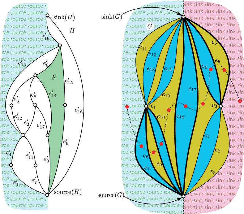
Next, let be an upward bipolar plane graph. The arcs of divide the plane into regions. Exactly one of these regions is geometrically unbounded; we call the rest of the regions inner facets. Take a Jordan curve such555We stipulate that has exactly one point at infinity and, if possible, is a projective line. that connects and in the projective plane and the affine part (the set of those points of that are not on the line at infinity) lies in the unbounded region. Then divides the unbounded region into two parts called outer facets . In Figure 2, is the union of the two thick dotted half-lines. The facets of are its inner facets and the two outer facets. In Figure 2, any two facets of sharing an arc are indicated by different colors (or by distinct shades in a grey-scale version).
Definition 3.
For an upward bipolar plane graph , we define the dual of , which we denote by , in the following way. Let be the set of all facets of , including the two outer facets. For each edge , we define the dual edge , as follows. Let and be the two facets such that the arc is on their boundaries. Out of these two facets, is the one on the left when we walk along from to 666Miller and Naor [10] call this the “left-hand rule”, since if our left thumb points in the direction of , then the left index finger shows the direction of ., while the other facet is . The edge set of is . In Figure 2, and are the left outer facet and the right outer facet. (Only a bounded part of each of these two geometrically unbounded facets is drawn.) Note that occurring before this definition belongs neither to nor to .
Note that there are isomorphic upward bipolar plane graphs and such that and are non-isomorphic; this is why we cannot define the dual of an upward bipolarly oriented planar graph. Observe that the dual of an upward bipolar plane graph is a bipolar graph777This is why Definition 3 deviates from the literature, where has only one outer facet, the outer region. Fact 1, to be formulated later, asserts more., so the following definition makes sense.
Definition 4.
With upward bipolar plane graphs and , let , , be a paired-bipolar-graphs problem; see (3.5). Define the bijections and by and , respectively, for ; here and are edges of the dual graphs defined in Definition 3. Then the dual of the paired-bipolar-graphs problem is the paired-bipolar-graphs problem
| (4.1) |
Briefly and roughly saying, we obtain the dual problem by interchanging the two graphs and dualizing both.
Theorem 1.
Let , , be a paired-bipolar-graphs problem such that both and are upward bipolar plane graphs. Then and the dual problem have exactly the same solutions.
This theorem, to be proved soon, trivially implies the following statement.
Corollary 1.
For , , , , , and as in Theorem 1 and for every , , , is a paired-bipolar-graphs scheme if and only if so is , , .
An arc in the plane is strictly ascending if for all . A plane graph is ascending if all its arcs are strictly ascending. Platt [11] proved888Indeed, as and are on , we can connect them by a new arc without violating planarity. Furthermore, we can add parallel arcs to any arc. Thus, Platt’s result applies. the following result, mentioned also in Auer at al. [1].
Theorem 2 (Platt [11]).
Each upward bipolar plain graph is isomorphic to an upward bipolar ascending plain graph.
Proof of Theorem 1.
Let and be as in the theorem. Theorem 2 allows us to assume that and are upward bipolar ascending plain graphs; see Figure 1 for an illustration. As the graphs are ascending, Figure 1 satisfactorily reflects generality. Note that the summation in (3.4) does not depend on the order in which the edges of a directed path are listed. Hence, we often give a directed path by the set of its edges. We claim that for any nonempty ,
| (4.2) |
For , this is clear by (3.3). The case and (3.4) imply the general case of (4.2), since
and the two summations after the equality sign above can be interchanged.
Assume that is a solution of . To show that is a solution of , too, take a maximal directed path in . In Figure 2, , , and, furthermore, consists of the thick edges of . Note that (3.1), with instead of , is valid for . Denote by the set of vertices of path ; it consists of some facets of . To mark these facets in the figure and also for a later purpose, for each facet , we pick a point called capital999Since we think of the facets as path-connected countries on the map. in the geometric interior of . These capitals are the red pentagon-shaped points in Figure 2. We assume that the capital of , the left outer facet, is far on the left, that is, its abscissa is smaller than that of every vertex of . Similarly, the capital of is far on the right. We need to show that
| (4.3) |
are the same. So we need to show that for all , .
First, we deal with the case when is an internal facet of ; see on the left of Figure 2. As is ascending, the set of arcs on the boundary of is partitioned into a left half and a right half . Furthermore, all arcs on (as well as in ) are ascending. Let belongs to and belongs to . In Figure 2, and . For a directed path , let and denote the tail of the first edge and the head of the last edge of , respectively.
For later reference, we point out that this paragraph to prove (the forthcoming) (4.6) uses only the following property of and : the directed paths
| (4.4) |
Take a subset such that and is a maximal directed path in . In Figure 2, . Note that and is also a maximal directed path in . As is a solution of , , ,
| (4.5) |
simply because both are . By (3.4), both sides of (4.5) are sums. Subtracting from both sides, we obtain that
| (4.6) |
Connect the capitals of the facets belonging to by an open Jordan curve such that for each , the arc and have no geometric point in common and, furthermore, for each , and has exactly one geometric point in common and this point is neither nor . In Figure 2, is the thin dashed curve. Let is (geometrically) below . Similarly, let be the set of those vertices of that are above . Note that and . In Figure 2, and . Consider the sum
| (4.7) | ||||
| (4.8) |
where the first equality comes from (3.4). If , , then
in virtue of (3.3), eliminate each other in the inner summation in (4.8). If , , then does not influence the inner summation at all. As is ascending, the case and does not occur. So (4.8) depends only on those for which and . However, by the definitions of , , , , and , these subscripts are exactly the members of . Thus, we can change in (4.8) to . For such an , only is in and, by (3.3), only contributes to the inner summation in (4.8). Therefore, we conclude that
| (4.9) |
As and have played the same role so far, we also have that
| (4.10) |
Therefore, combining (4.6), (4.9), and (4.10), we obtain that
| (4.11) |
For and , by the left-hand rule quoted in Footnote 6, and . So, at the sign below, we can use (3.3) and that is not the endpoint of any further edge of . Using (3.4), (4.3), (4.9), and (4.10), too,
| (4.12) | |||
| (4.13) | |||
| (4.14) |
Next, we deal with the case . So is the outer facet left to ; see Figure 2. We modify the earlier argument as follows. Let is on the left boundary of . In Figure 2, , , , . Now is the set of outgoing edges from in . As is a maximal directed path in ,
| (4.15) |
Similarly to (4.7)–(4.8), we take the sum
| (4.16) |
Like earlier, the inner sum in (4.16) is 0 unless and , that is, unless . Thus, we can change the range of the outer sum in (4.16) from to ; note that in Figure 2. For , the inner sum is . Therefore, (4.16) turns into
| (4.17) |
So (4.17), (4.15), (3.2), , and imply that
| (4.18) |
Similarly to (4.14), but now there is no incoming edge into and so “the earlier ” is and not needed, we have that
| (4.19) | |||
| (4.20) |
By (4.20) and (4.18), . Since by (3.2) and (4.3), we obtain the required equality .
The treatment for the remaining case could be similar, but we present a shorter approach. By (3.2), (4.3), and the dual of (4.2),
| (4.21) |
We already know that for each except possibly for , on the left of (4.21) equals the corresponding summand on the right. This fact and (4.21) imply that , as required.
After settling all three cases, we have shown that and in (4.3) are the same. This proves that any solution of is also a solution of .
To prove the converse, we need the following easy consequence of Platt [11].
Fact 1 (Platt [11]).
If is an upward bipolar plane graph, then its dual, , is isomorphic to an upward bipolar plain graph.
We can extract Fact 1 from Platt [11] as follows. As earlier but now for each facet of , pick a capital in the interior of . For any two neighboring facets and , connect and by a new arc through the common bordering arc of and . The capitals and the new arcs form a plane graph isomorphic to , in notation, . As is an upward bipolar plain graph by Definition 2, we obtain Fact 1.
Temporarily, we call the way to obtain from above a prime construction; the indefinite article is explained by the fact that the vertices and the arcs of can be chosen in many ways in the plane. The transpose of a graph is obtained from by reversing all its edges. For , stands for the transpose of ; note that , , and .
Resuming the proof of Theorem 1, Theorem 2 allows us to assume that and are ascending. Let be a plane graph obtained from by a prime construction; is isomorphic to . In Figure 2, only some vertices of are indicated by red pentagons and only some of its arcs are drawn as segments of the thin dashed open Jordan curve, but the figure is still illustrative. To obtain a graph isomorphic to , we apply a prime construction to so that the vertices of are the chosen capitals that form and, geometrically, the original arcs of are the chosen arcs of connecting these capitals. By the left-hand rule quoted in Footnote 6, is . Hence . Similarly, . Let us define and in the natural way by and . We claim that
| (4.22) |
The reason is simple: to neutralize that the edges are reversed, a solution of should be changed to . However, the source and the sink are interchanged, and this results in a second change of the sign. So, a solution of is also a solution of . Similarly, a solution of is a solution of , proving (4.22).
Finally, let be a solution of . Fact 1 allows us to apply the already proven part of Theorem 1 to instead of , and we obtain that is a solution of . We have seen that and . Apart from these isomorphisms, and are and , respectively. Thus, and have the same solutions. Hence is a solution of , and so (4.22) implies that is a solution of , completing the proof of Theorem 1. ∎
Remark 1.
Apart from applying the result of Platt [11], the proof above is self-contained. Even though Platt’s result may seem intuitively clear, its rigorous proof is not easy at all. Since a trivial induction instead of relying on Platt [11] would suffice for the particular graphs occurring in the subsequent section, our aim to give an elementary proof of Hutchinson’s self-duality theorem is not in danger.
5. Hutchinson’s self-duality theorem
The paragraph on pages 272–273 in [9] gives a detailed account on the contribution of each of the two authors of [9]. In particular, the self-duality theorem, to be recalled soon, is due exclusively to George Hutchinson. Thus, we call it Hutchinson’s self-duality theorem, and we reference Hutchinson [9] in connection with it. A similar strategy applies when citing his other exclusive results from [9].
The original proof of the self-duality theorem is deep. It relies on Hutchinson [8], which belongs mainly to the theory of abelian categories, on the fourteen-page-long Section 2 of Hutchinson and Czédli [9], and on the nine-page-long Section 3 of Hutchinson [9]. A second proof given by Czédli and Takách [6] avoids Hutchinson [8] and abelian categories, but relying on the just-mentioned Sections 2 and 3, it is still complicated. No elementary proof of Hutchinson’s self-duality theorem has previously been given; in light of Remark 1, we present such a proof here.
By a module over a ring with we always mean a unital left module, that is, holds for all . The lattice of all submodules of is denoted by . For , and means and , respectively, while is the submodule generated by . A lattice term is built from variables and the operation symbols and . For lattice terms and , the string “” is called a lattice identity. For example, is a lattice identity; in fact, it is one of the two (equivalent) distributive laws. To obtain the dual of a lattice term, we interchange and in it. For example, the dual of
| (5.1) | ||||
| (5.2) | ||||
The dual of a lattice identity is obtained by dualizing the lattice terms on both sides of the equality sign. For example, the dual of the above-mentioned distributive law is , the other distributive law.
Now we can state Hutchinson’s self-duality theorem.
Theorem 3 (Hutchinson [9, Theorem 7]).
Let be a ring with , and let be a lattice identity. Then holds in for all unital modules over if and only if so does the dual of .
Even the following corollary of this theorem is interesting. For , let be the class of Abelian groups101010We note but do not need that the s are exactly the varieties of Abelian groups. satisfying the identity with summands on the left. In particular, is the class of all Abelian groups.
Corollary 2 (Hutchinson [9]).
For and any lattice identity , holds in the subgroup lattices of all if and only if so does the dual of .
By treating each as a left unital module over the residue-class ring in the natural way, Corollary 2 follows trivially from Theorem 3.
Proof of Theorem 3.
We can assume that is of the form where and are lattice terms. Indeed, any identity of the form is equivalent to the conjunction of and . Thus, from now on, by a lattice identity we mean a universally quantified inequality of the form
| (5.3) |
The dual of , denoted by , is , where and are the duals of the terms and , respectively. Let us call in (5.3) a -balanced identity if every variable that occurs in the identity occurs exactly once in and exactly once in . For lattice identities and , we say that and are equivalent if for every lattice , holds in if and only if so does . As the first major step in the proof, we show that for each lattice identity ,
| (5.4) |
To prove (5.4), observe that the absorption law allows us to assume that every variable occurring in occurs both in and . Indeed, if occurs, say, only in , then we can change to . Let be the set111111(5.3) allows variables only from , so is a set. As usual, . of those lattice identities in (5.3) for which (5.4) fails but the set of variables occurring in is the same as the set of variables occurring in . We need to show that . Suppose the contrary. For an identity belonging to , let be the number of those variables that occur at least three times in (that is, more than once in or ). The notation comes from “badness”. Pick a member of that minimizes . As , we know that . Let be the set of variables of . As remains the same when we permute the variables, we can assume that occurs in at least three times. Let and denote the number of occurrences of in and that in , respectively; note that and . Clearly, there is a -ary term , …, , , …, such that each of , …, occurs in exactly once and is of the form
where is listed times in and . For example, if
then we can let
Similarly, there is an -ary term , …, , , …, such that each of , …, occurs in exactly once and is of the form
where is listed times in and is still Consider the -by- matrix of new variables; it has rows and columns. Let
be the vector of variables formed from the elements of . That is, to obtain , we have listed the entries of row-wise. We define the -ary terms
and we let . As each of the s occurs in each of and exactly once and the numbers of occurrences of did not change, . So, by the choice of , we know that is outside . Thus, is equivalent to a 1-balanced lattice identity.
Next, we prove that is equivalent to . Assume that holds in a lattice . Letting all the s equal and using the fact that the join and the meet are idempotent operations, it follows immediately that also holds in . Conversely, assume that holds in , and let the s and denote arbitrary elements of . Since the lattice terms and operations are order-preserving, we obtain that
showing that holds in . So is equivalent to . Hence, is equivalent to a -balanced identity, since so is . This contradicts that and proves (5.4).
Clearly, if is equivalent to a 1-balanced lattice identity , then the dual of is equivalent to the dual of , which is again a 1-balanced identity. Thus, it suffices to prove Theorem 3 only for 1-balanced identities. So, in the rest of the paper,
| (5.5) |
lattice identity.
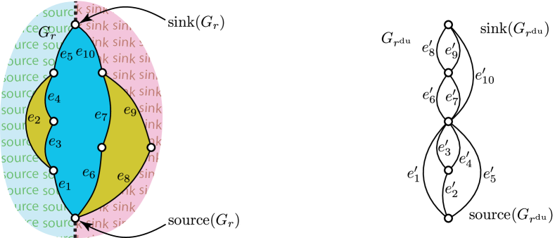
For a lattice term , will stand for the set of variables occurring in . We say that is repetition-free if each of its variables occurs in only once, that is, if is -balanced. With the lattice terms given (5.1) and (5.2), the following definition is illustrated by Figure 3.
Definition 5.
With each repetition-free lattice term , we are going to associate an upward bipolar ascending plane graph up to isomorphism and a bijection by induction as follows. If is a variable, then is the two-element upward bipolar plane graph with a single directed edge, and is the only possible bijection from the singleton to the singleton . For , we obtain by putting atop and identifying (in other words, gluing together) and . Then and . For , we obtain by bending or deforming, resizing, and moving and so that , , and the rest of is on the left of the rest of . Then and . If or , then let , that is, for and , .
In the aspect of , the lattice operations are associative but not commutative. A straightforward induction yields that for every lattice term ,
| (5.6) | |||
| (5.7) |
(5.6) and (5.7) are exemplified by Figure 3, where is given by facets.
The ring with 1 in the proof is fixed, and is its additive group. For in (5.5), we denote by the set of systems of contents of with respect to . That is, complying with the terminology of Definition 1(pb2),
| (5.8) |
For a unital module over (an -module for short), similarly to (5.8), let
Interrupting the proof of Theorem 3, we formulate and prove two lemmas.
Lemma 1.
For submodules , …, and elements of an -module , if and only if there exists an such that
| (5.9) |
for all edge . The same holds with and instead of and , respectively.
Letting , the lemma describes the containment . However, now that the lemma is formulated with , it will be easier to apply it later. Based on the rule that for , , we have that if and only if there is a such that and . (For the “only if” part: .) Hence, the lemma follows by a trivial induction on the length of ; the details are omitted. Alternatively (but with more work), one can derive the lemma from the congruence-permutable particular case of Czédli [2, Claim 1], [3, Proposition 3.1], [4, Lemma 3.3] or Czédli and Day [5, Proposition 3.1] together with the canonical isomorphism between and the congruence lattice of . The following lemma, in which and are defined in Definition 5, is crucial and less obvious.
Lemma 2.
Let be a ring with and let be a -balanced lattice identity as in (5.5). Then the following two conditions are equivalent.
-
(1)
For every (unital left) -module , holds in .
-
(2)
, , has a solution.
Proof of Lemma 2.
For , we denote and by and , respectively.
Assume that (1) holds. Let be the free unital -module121212We note but do not use the facts that can be treated an -module denoted by , and that we are defining is the th direct power of . generated by . For each , let be the submodule generated by . In other words, . Taking defined by (like an identity map) for , Lemma 1 implies that . So, as we have assumed (1), . Therefore, Lemma 1 yields a system of contents such that , , and for every , . Thus, for each , we can pick an such that
| (5.10) |
Let stand for the paired-bipolar-graphs problem occurring in (2). With the s in (5.10), let . We claim that is a solution of . To show this, let , …, be a maximal directed path in . Let us compute, using the equality for at and (5.10) at :
| (5.11) | |||
| (5.12) | |||
| (5.13) |
For , define and and and . Expressing (5.13) as a linear combination of the free generators of with coefficients taken from , the coefficient of is . Hence, it follows from (3.3) and (3.4) that
| (5.14) | ||||
| (5.15) |
is the coefficient of in (5.13) and, by (5.11), also in the linear combination expressing . On the other hand, the coefficients of , , and , in the straightforward linear combination expressing are , , and , respectively. Since is freely generated by , this linear combination is unique. Therefore, (5.15) is , , and for , , and , , respectively. Thus, the function applied on the right of (5.15) to is the same as defined in (3.2). As this holds for all , the just-mentioned function equals . Hence, is a solution of ; see (3.6). We have shown that (1) implies (2).
To show the converse implication, assume that (2) holds, and let be a solution of . Let be an -module, let , and let . It is convenient to let ; then we obtain an satisfying (5.9) for all . Note in advance that when we reference Section 4, , , and . For each ,
| (5.16) |
here depends on the choice of this path (and on ). With reference to (3.4), let
| (5.17) |
We know from Section 4 that (4.4) implies (4.6). Hence, the coefficient of in (5.17) does not depend on the choice of . Thus, is well defined, that is
| (5.18) |
As in (5.17) belongs to and its coefficient to , . So, . As the empty sum in is , we have that . Since is a solution of and is a maximal directed path in , it follows from (5.17), (3.6), (3.2), and (5.9) that
To see the third part of (5.9) with and instead of and , let . According to (5.16) but with instead of , let be the chosen directed path for . By (5.18), we can assume that is obtained from by adding to its end. So , ,
Hence, applying (3.4) to the coefficient of each of the in (5.17),
| (5.19) |
As and most of the summands above are zero by (3.3), (5.19) turns into
which belongs to since satisfies (5.9). Thus, Lemma 1 yields that . Therefore, , that is, (1) holds, completing the proof of Lemma 2. ∎
Next, we resume the proof of Theorem 3. As noted in (5.5), is 1-balanced. Clearly, so is . Letting is an -module and , , , Lemma 2 gives that
| (5.20) |
Tailoring Definition 4 to the present situation, define and , …, in the natural way by and . With , , , Lemma 2 yields that
| (5.21) |
Let denote the dual of ; see Definition 4. It follows from (5.6)–(5.7) and Definitions 3 and 4 that is the same as . Hence, (5.21) turns into
| (5.22) |
Finally, Theorem 1, (5.20), and (5.22) imply that holds in if and only if so does , completing the proof of Theorem 3. ∎
References
- [1] C. Auer, C. Bachmier, F. Brandenburg, A. Gleissner, K. Hanauer: Upward planar graphs and their duals. Theoretical Computer Science 571, 36–49 (2015) http://dx.doi.org/10.1016/j.tcs.2015.01.003
- [2] G. Czédli: A characterization for congruence semi-distributivity. Proc. Conf. Universal Algebra and Lattice Theory, Puebla (Mexico, 1982), Springer-Verlag Lecture Notes in Math. 1004, 104–110.
- [3] G. Czédli: Mal’cev conditions for Horn sentences with congruence permutability, Acta Math. Hungar. 44 (1984), 115–124
- [4] G. Czédli: Horn sentences in submodule lattices. Acta Sci. Math. (Szeged) 51 (1987), 17–33
- [5] G. Czédli, A. Day: Horn sentences with (W) and weak Mal’cev conditions. Algebra Universalis 19, (1984), 217–230
- [6] G. Czédli, G. Takách: On duality of submodule lattices, Discussiones Matematicae, General Algebra and Applications 20 (2000), 43–49.
- [7] G. Di Battista, P. Eades, R. Tamassia, I.G. Tollis: Algorithms for drawing graphs: an annotated bibliography. Computational Geometry 4 (1994), 235–282. https://doi.org/10.1016/0925-7721(94)00014-X
- [8] G. Hutchinson: A duality principle for lattices and categories of modules. J. Pure and Applied Algebra 10 (1977) 115–119.
- [9] G. Hutchinson, G. Czédli: A test for identities satisfied in lattices of submodules. Algebra Universalis 8, (1978), 269–309
- [10] G.L. Miller, J. Naor: Flow in planar graphs with multiple sources and sinks. SIAM J. Comput. 24/5. 1002–1017, October 1995
- [11] C.R. Platt: Planar lattices are planar graphs. J. Combinatorial Theory (B) 21, 30–39 (1976)