Dynamic analysis of influential stocks based on conserved networks

Let $p_{i}(\tau)$ $(i=1,2,\cdots,N;\tau=1,2,\cdots,M)$ be the daily closing price of stock $i$ at time $\tau$, one obtains the logarithmic return of $i$ over a time interval $\Delta\tau$ by

$$r_{i}(\tau)=\ln p_{i}(\tau)-\ln p_{i}(\tau-\Delta\tau).$$

(1)

In this paper we set $\Delta\tau=1$, so $r_{i}(\tau)$ represents the daily return of stock $i$ at time $\tau$. Then, the correlation coefficient between stocks $i$ and $j$ is defined by

$$w_{ij}=\frac{\langle r_{i}r_{j}\rangle-\langle r_{i}\rangle\langle r_{j}\rangle}{\sigma_{i}\sigma_{j}},$$

(2)

where $\langle r_{i}\rangle=\sum_{\tau=1}^{M}r_{i}(\tau)/M$ is the mean and $\sigma_{i}=\sqrt{\sum_{\tau=1}^{M}\left[r_{i}-\langle r_{i}\rangle\right]^{2}/M}$ is the standard deviation. The ensemble of $w_{ij}$ forms the correlation matrix $\bm{W}$ of a stock market in a window of width $M$.

To filter $w_{ij}$, we use the P-threshold method and set the following hypothesis test [22],

	$\displaystyle H_{0}:$	$\displaystyle w_{ij}=0,$			(3)
	$\displaystyle H_{1}:$	$\displaystyle w_{ij}\neq 0.$			(4)

The corresponding test statistic is

$$T_{ij}=w_{ij}\sqrt{\frac{n-2}{1-w_{ij}^{2}}}\sim t_{n-2},$$

(5)

where $n$ is the sample size and $n-2$ is the degree of freedom. Given a significance level $\alpha$, one should reject $H_{0}$ if the absolute value of the test statistic exceeds the cut-off value $t_{\alpha/2}(n-2)$, namely, if

$$|T_{ij}|>t_{\alpha/2}(n-2).$$

(6)

To maximize the number of discoveries while controlling the fraction of false discoveries, we perform the multiple hypothesis test based on the Bonferroni correction. Specially, for the significance level of $\alpha=0.01$, we include any interactions between stocks if $|T_{ij}|>t_{\alpha/N(N-1)}(n-2)$. Since the Bonferroni correction assumes complete independence between the tested p-values, one may consider further the False Discovery Rate (FDR) approach [31] to relax the assumption of independence. As a consequence, more edges among stocks will be maintained. For smoothing purpose, we adopt the moving-window method [32]. Assuming the width of each window is $M$ and the sliding interval is $\Delta M$, one can obtain a series of windows overlap with each other for any oberving period with proper choices of $M$ and $\Delta M$. Inside each window, an edge is created between a pair of stocks $i$ and $j$ if $w_{ij}\neq 0$. This process is repeated throughout all the elements of the correlation matrix and finally a stock network is generated. Specially, we assume the network $G(V,E)$ is unweighted and undirected, which can be described by an adjacency matrix $\bm{A}=(a_{uv})_{N\times N}$ with elements

$$a_{uv}=\biggl{\{}\begin{array}[]{ll}1,&\quad\mbox{if $u$ and $v$ are connected,}\\ 0,&\quad\mbox{otherwise.}\end{array}$$

(7)

A typical stock market usually experiences various financial situations, including bull and bear runs, business as usual and financial crises. Of great importance is to delve into reliable indicators of the crisis from the market. However, the 2008 financial crisis has highlighted the main limitations of standard models, as they cannot detect the crisis even by using posterior data [33]. Here, we address this issue by means of conserved networks. According to different states associated with a crisis, we divide the whole investigating period into $5$ stages: the normal stage before the crisis, the stage of the transition from the normal state to the crisis, the stage during the crisis, the stage of the transition from the crisis to the normal state and the stage after the crisis. Inside any stage, there are a number $K$ of consecutive windows overlap with each other, based on which $K$ stock networks are constructed. Furthermore, we assume that the interactions between significant stocks will persist while the interactions between insignificant stocks will vary with time, which leads to the idea of conserved networks: for any pair of stocks, an edge between them in the corresponding conserved network exists if and only if all these $K$ networks within the stage have this edge. As a consequence, we obtain $5$ conserved networks, which characterize dynamic characteristics of the investigating period.

The most influential stocks may help us understand risk propagation in a stock market and design corresponding control measures. To represent nodal influence in each conserved network, we adopt the concept of centrality. In this paper, we consider four typical measures: degree centrality (DC), eigenvector centrality (EC), closeness centrality (CC) and betweenness centrality (BC).

Given a stock network $G(V,E)$, the DC of node $u\in V$ is define by [34]

$$\texttt{DC}(u)=k_{u},$$

(8)

where $k_{u}=\sum_{v=1}^{|V|}a_{uv}$ is the degree of node $u$ and $|V|$ is the number of nodes. Although the DC is the simplest centrality measure, it can be illuminating. In stock markets, it seems reasonable to suppose that stocks with connections to many others might have more access to information than those with fewer connections. A natural extension of the DC is EC, defined as [35]

$$\texttt{EC}(u)=\bm{\upsilon}_{u}^{\texttt{max}},$$

(9)

where $\bm{\upsilon}^{\texttt{max}}$ is the eigenvector corresponding to the largest eigenvalue of the adjacency matrix $\bm{A}$ and $\bm{\upsilon}_{u}^{\texttt{max}}$ is the $u$th element of $\bm{\upsilon}^{\texttt{max}}$ corresponding to stock $u$. As a consequence, the stock $u$ with larger $\texttt{EC}(u)$ can be important because it has many neighbors (even though those stocks may not be important themselves) or because it has important neighbors of high degrees.

Both the DC and EC only consider local information of a network. Regarding global information, some entirely different measures of centrality have been suggested incorporating shortest path lengths. One is CC, defined as [34]

$$\texttt{CC}(u)=\frac{|V|-1}{\sum_{v\in V}l(u,v)},$$

(10)

where $l(u,v)$ is the shortest path length from node $u$ to node $v$. According to Eq. (10), the smaller average distance from the stock $u$ to others, the larger value of $\texttt{CC}(u)$ it has. BC is another different concept of centrality, initially proposed by Bavelas [36] and generalized by Freeman [37],

$$\texttt{BC}(u)=\frac{\eta(s,u,t)}{\sum_{s\neq u\neq t}\eta(s,t)},$$

(11)

where $\eta(s,u,t)$ is the number of those shortest paths passing through $u$ and $\eta(s,t)$ is the total number of the shortest paths from node $s$ to node $t$. In contrast to the CC, the BC measures the extent to which a stock lies on paths between other stocks.

Different centrality measures yield different ranks of nodal influence. To synthesize multiple centralities, we regard each rank as an order statistic [38] and obtain a Q-statistic from the joint cumulative distribution of the $n$-dimensional order statistic:

$$Q(\gamma_{1},\gamma_{2},\cdots,\gamma_{n})=n!\int_{0}^{\gamma_{1}}\int_{q_{1}}^{\gamma_{2}}\cdots\int_{q_{n-1}}^{\gamma_{n}}\texttt{d}q_{n}\texttt{d}q_{n-1}\cdots\texttt{d}q_{1},$$

(12)

where $\gamma_{i}$ is the rank ratio for centrality $i$ and $q_{i}$ is the lower bound of the $(i+1)$th order statistic. In present work, we use $4$ centrality measures, hence $n=4$. In fact, the above integration can be calculated in a fast way

$$Q(\gamma_{1},\gamma_{2},\cdots,\gamma_{n})=n!Q_{n}$$

(13)

with $Q_{k}=\sum_{i=1}^{k}(-1)^{i-1}Q_{k-i}\gamma_{k-i+1}^{i}/i!$. The larger value of $Q$, the greater influence the node has.

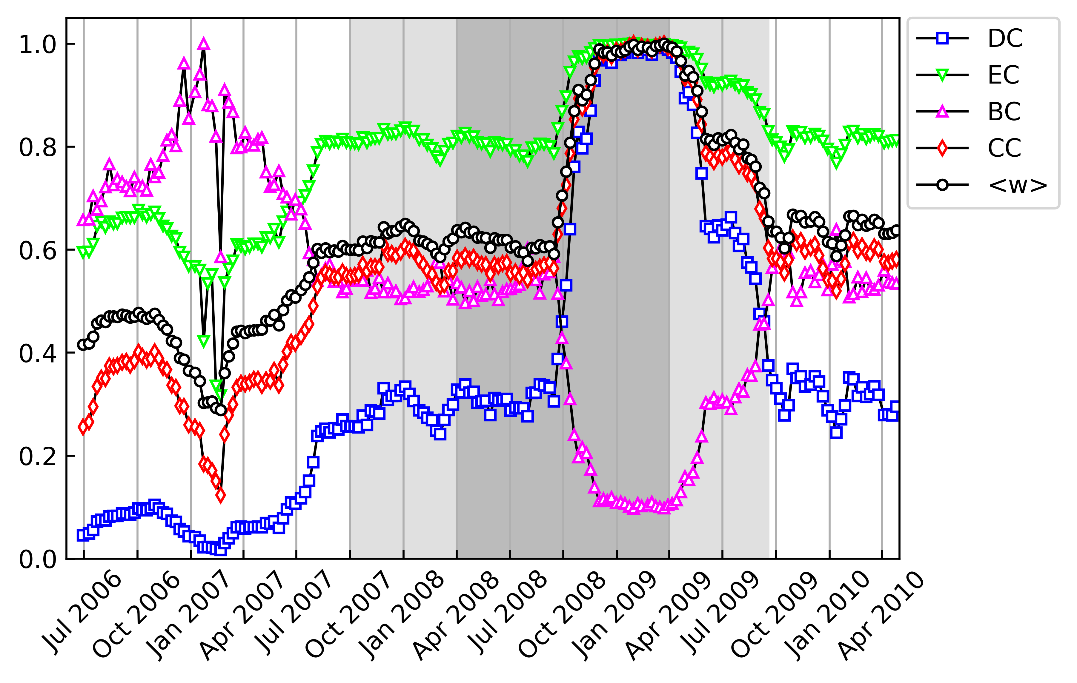
First of all, we divide the investigated period through moving windows. By setting the width of each window as $M=125$ (about half a year) and the moving step as $\Delta M=5$ (about a week), we obtain $193$ windows. For each window, we fix the significance level at $\alpha=0.01$, based on which a correlation network is constructed. As a result, we obtain $193$ consecutive networks for the whole period. Then, we calculate the centrality of each node, the average of which is used to stand for the characteristics of the network. For each network, we consider the DC, EC, CC and BC, respectively. Figure 1 shows the evolution of four centralities in comparison to the evolution of the average correlation coefficient $\langle w\rangle$. For comparison, we normalize each plot by the corresponding maximum of the investigating period. However, it is not essential. The dark gray interval corresponds to the middle stage of the crisis and the two light gray intervals respectively correspond to the early transition from the normal state to the crisis and the late transition from the crisis to the normal state. Remarkably, the DC, EC and CC display the same trend with $\langle w\rangle$, while the BC evolves in the opposite way. According to Eq. (8), one has $\langle\texttt{DC}\rangle=\sum_{u\in V}k_{u}/|V|=2|E|/|V|=(|V|-1)e$, where $|E|$ is the number of edges and $e=2|E|/|V|/(|V|-1)$ is the density of edges. Moreover, the edge density is proportional to $\langle w\rangle$. Therefore, both the DC and EC exhibit the same trend as $\langle w\rangle$. As to the CC and BC (see Eqs. (10) and (11)), the higher density of edges, the smaller distance that a node reach all the others, hence the larger value of the CC. On the contrary, the number of connected pairs of nodes increases, resulting in the decrease of the BC. Overall, the four measures can serve as good indicators of the market evolution from the macro perspective.

Considering the 2008 financial crisis, we divide the period from January 2006 to April 2010 into $5$ stages: the normal stage before the crisis, the stage of the transition from the normal state to the crisis, the stage during the crisis, the stage of the transition from the crisis to the normal state and the stage after the crisis. For each stage, we generate a conserved network. Table 1 shows the basic characteristics of the $5$ conserved networks, including the number of stocks $N$, the number of edges $E$, the average degree $\langle k\rangle$, the average clustering coefficient $\langle c\rangle$ and the average shortest path length $\langle l\rangle$. One notices apparent differences between these networks. For instance, the conserved network in the crisis is relatively dense because of the higher systemic risk. As a result, $\langle k\rangle$ and $\langle c\rangle$ are larger while $\langle l\rangle$ is smaller. But these topologies only provide macro information of the market development.

The 2008 financial crisis is due to the U.S. financial problem of subprime mortgages. Mortgage is a loan taken from bank to buy a house, which is an agreement between homebuyers and banks. In general, people with low credit and low income can not get a loan from retail banks. But since year 2000’s, a third party got involved, namely investment banks. These investment banks started buying mortgage agreements from the retail banks. In this way, the retail banks sold the loans to investment banks to have zero liability and the mortgages bought by the investment banks were used to form Mortgage Backed Security. Although the Mortgage Backed Security is a special category of subprime mortgages with higher risk, it yields higher return at the same time. As more people were becoming eligible for the mortgage, the demand for homes started increasing. More people had money (borrowed) to buy a new home. The price of residential properties only went up, hence creating the bubble. Table 2 lists $10$ most influential stocks identified from the conserved network corresponding to the normal stage before the crisis (from June 30th 2006 to September 25th 2007). As is expected, $6$ stocks are from the real estate sector.

Investment banks made the loans were issued to people who had little capability to payback the loan. Inevitably, some of them eventually could not afford the monthly payments and their property went for foreclosure. At a point in 2007-2008, there were more houses on sale than there were buyers for it. This triggered a steady price fall. The housing bubble burst. When property prices started going down, people who had bought the property with the sole purpose of “buying low and selling high”stopped paying the mortgage. This led to more loan defaults and more foreclosures. As a result, the share price of the Mortgage Backed Security started to fall continuously and eventually started to affect on big investors that could not cover this urgency. So the crisis came into being. Table 3 lists $10$ most influential stocks identified from the conserved network corresponding to the early transition from the normal state to the crisis (from October 2nd 2007 to Marc 26th 2008), among which $6$ stocks are financials, indicating the first shock of the crisis.

After the burst of the bubble in the housing market, many investment banks had more liabilities than assets and faced a big trouble of liquidity. For example, the New Century Financial Corporation filed for Chapter 11 bankruptcy protection in April 2008 because of repurchase agreements and the Lehman Brothers announced bankrupt in September 2008 due to asset deterioration. In addition to investment banks, many insurance companies and financial institutions have also been greatly impacted. A conspicuous example is the American International Group, which lost $250$ billion dollars in the second quarter of 2008 and was taken over by the U.S. government finally. Soon after the earthquake in the financial market, the real economy was also shocked. On the one hand, the depression of the housing market caused correlated companies to fold. One the other hand, the rising unemployment and the shrink of personal wealth decreased consuming intention for industrial products. Table 4 lists $10$ most influential stocks identified from the conserved network corresponding to the stage during the crisis (from April 2nd 2008 to March 30th 2009). We find that not only financial institutions but also correlated industrial companies were involved with enormous losses.

To contain the crisis, the Troubled Assets Relief Program was carried out in October 2008, which authorized the United States Treasury to spend up to $700$ billion dollars to purchase trouble assets both domestically and internationally. The act was widely credited with restoring stability and liquidity to the financial sector, unfreezing the markets for credit and capital and lowering borrowing costs for households and businesses. This, in turn, helped restore confidence in the financial system and restart economic growth. Another dose of fiscal stimulus is monetary easing. The lower interest rate spurred businesses to make new investments, spurred industrials to invest in renovations and spurred purchases of major durable goods like cars. Table 5 lists $10$ most influential stocks identified from the conserved network corresponding to the late transition from the crisis to the normal state (from April 6th 2009 to September 18th 2009), among which $8$ stocks are industrials, implying the initial recovery.

In fact, the speed of the recovery from the 2008 financial crisis has been unusually slow. Nevertheless, under the percolation of the stimulating policy of quantitative easing, the U.S. economy began to recover since the middle of 2009. With the reduction of the systematic risk and the rising opportunity for business, the stock market boomed again. Table 6 lists $10$ most influential stocks identified from the conserved network corresponding to the stage after the crisis (from September 25th 2009 to April 26th 2010), suggesting that the market is active across various sectors, including financials, industrials, materials, real estate and energy.

References

- [1] Mantegna R N and Stanley H E 2000 An Introduction to Econophysics: Correlations and Complexity in Finance (Cambridge: Cambridge University Press)
- [2] Campbell J, Lo A W and MacKinlay A C 1997 The Econometrics of Financial Markets (Princeton: Princeton University Press)
- [3] Laloux L, Cizeau P, Bouchaud J P and Potters M 1999 Phys. Rev. Lett. 83 1467
- [4] Plerou V, Gopikrishnan P, Rosenow B, Amaral L A N and Stanley H E 1999 Phys. Rev. Lett. 83 1471
- [5] Potters M and Bouchaud J P 2021 A First Course in Random Matrix Theory (Cambridge: Cambridge University Press)
- [6] Eom C, Oh G, Jung W S, Joeng H and Kim S 2009 Physica A 388 900
- [7] Song D M, Tumminello M, Zhou W X and Mantegna R N 2011 Phys. Rev. E 84 026108
- [8] Jiang X F, Chen T T and Zheng B 2014 Sci. Rep. 4 5321
- [9] Wang D, Zhang X, Horvatic D, Podobnik B and Stanley H E 2017 Chaos 27 023104
- [10] Djauhari M A and Gan S L 2016 J. Stat. Mech. 093401
- [11] Newman M E J 2003 SIAM Rev. 45 167
- [12] Bonanno G, Caldarelli G, Lillo F and Mantegna R N 2003 Phys. Rev. E 68 046130
- [13] Onnela J P, Kaski K and Kertesz J 2004 Eur. Phys. J. B 38 353
- [14] Tumminello M, Aste T, Di Matteo T and Mantegna R N 2005 Proc. Natl. Acad. Sci. USA 102 10421
- [15] Boginski V, Butenko S and Pardalos P M 2005 Comput. Statist. Data Anal. 48 431
- [16] Tumminello M, Di Matteo T, Aste T and Mantegna R N 2007 Eur. Phys. J. B 55 209
- [17] Liu J, Tse C K and He K 2011 Quant. Finance 11 817
- [18] Wang G J, Xie C and Chen S 2017 J. Econ. Interact. Coord. 12 561
- [19] Xu X J, Wang K, Zhu L and Zhang L J 2018 Physica A 509 1080
- [20] Wilinski M, Sienkiewicz A, Gubiec T, Kutner R and Struzik Z R 2013 Physica A 392 5963
- [21] Wilinski M, Ikeda Y and Aoyama H 2018 J. Stat. Mech 023405
- [22] Xu R, Wong W K, Chen G and Huang S 2017 Sci. Rep. 7 41379
- [23] Musciotto F, Marotta L, Piilo J and Mantegna R N 2018 Palgrave Commun. 4 92
- [24] Yang C, Shen Y and Xia B Y 2013 Mod. Phys. Lett. B 27 1350022
- [25] Bardoscia M, Livan G and Marsili M 2012 J. Stat. Mech. P08017
- [26] Bongiorno C and Challet D 2021 EPL 133 48001
- [27] Abhijit B, Chandrasekhar A G, Esther D and Jackson M O 2013 Science 341 1236498
- [28] Wang S, Schäfer R and Guhr T 2016 Eur. Phys. J. B 89 105
- [29] Benzaquen M, Mastromatteo I, Eisler Z and Bouchaud J P 2017 J. Stat. Mech. P023406
- [30] Roy R B and Sarkar U K 2011 Proc. of International Conference on Advances in Social Networks Analysis and Mining (Kaohsiung, Taiwan) pp 567
- [31] Benjamini Y and Hochberg Y 1995 J. Roy. Stat. Soc. B 57 449
- [32] Onnela J P, Chakraborti A, Kaski K, Kertész J and Kanto A 2003 Phys. Rev. E 68 056110
- [33] Stiglitz J E 2016 Towards a General Theory of Deep Downturns (Cambridge: Palgrave Macmillan)
- [34] Freeman L C 1978-1979 Soc. Netw. 1 215
- [35] Bonacich P F 1987 Am. J. Soc. 92 1170
- [36] Bavelas A 1948 Hum. Organ. 7 16
- [37] Freeman L C 1977 Sociometry 40 35
- [38] Dekking F M, Kraaikamp C, Lopuhaä H P and Meester L E 2005 A Modern Introduction to Probability and Statistics (London: Springer)
- [39] Langville A and Meyer C 2006 Google’s PageRank and Beyond: The Science of Search Engine Rankings (Princeton: Princeton University Press)
- [40] Mastromatteo I, Zarinelli E and Marsili M 2012 J. Stat. Mech. P03011
- [41] Squartini T, Caldarelli G, Cimini G, Gabrielli A and Garlaschelli D 2018 Phys. Rep. 757 1