Dynamic DH-MBIR for Phase-Error Estimation from Streaming Digital-Holography Data
Abstract
Directed energy applications require the estimation of digital-holographic (DH) phase errors due to atmospheric turbulence in order to accurately focus the outgoing beam. These phase error estimates must be computed with very low latency to keep pace with changing atmospheric parameters, which requires that phase errors be estimated in a single shot of DH data. The digital holography model-based iterative reconstruction (DH-MBIR) algorithm is capable of accurately estimating phase errors in a single shot using the expectation-maximization (EM) algorithm. However, existing implementations of DH-MBIR require hundreds of iterations, which is not practical for real-time applications.
In this paper, we present the Dynamic DH-MBIR (DDH-MBIR) algorithm for estimating isoplanatic phase errors from streaming single-shot data with extremely low latency. The Dynamic DH-MBIR algorithm reduces the computation and latency by orders of magnitude relative to conventional DH-MBIR, making real-time throughput and latency feasible in applications. Using simulated data that models frozen flow of atmospheric turbulence, we show that our algorithm can achieve a consistently high Strehl ratio with realistic simulation parameters using only 1 iteration per timestep.
Index Terms:
Coherent Imaging, Phase Retrieval, Atmospheric Turbulence, Digital Holography, Directed Energy, Wavefront SensingI Introduction
The goal of a directed energy system is to focus a beam of light on a distant object. In terrestrial applications, this can be difficult because atmospheric turbulence introduces random phase errors (or distortions) that tend to disperse the otherwise focused beam. A solution to this problem is to pre-distort the phase of the outgoing beam. This can be done by first performing wavefront sensing (WFS), in which the phase distortion of incoming light is measured. The outgoing light can then be pre-distorted with the conjugate phase. However, this approach requires that the WFS be performed with very low latency, so that the phase corrections can be used before the atmospheric distortion changes.
Traditionally, WFS is performed with a Shack-Hartmann wavefront sensor. However, since the Shack-Hartmann method is based on hardware, it is limited in speed and is effective only with moderate turbulence strength [1].
Alternatively, digital holography (DH) sensors can be used to estimate the wavefront from direct measurements of the light. DH sensors measure the amplitude and phase of incoming light by interfering the received light with a reference beam. The resulting complex-valued measurements can then be used to computationally estimate phase distortions by solving an inverse problem [2].
The Image Sharpening (IS) algorithm is one approach to estimating phase distortions from DH data [3]. This method is optimization-based and models the phase distortion with a Zernike expansion. However, the measured reflection from coherent light contains speckle [4], which reduces the effectiveness of the IS algorithm. A solution to this speckle problem is to take multiple shots of DH data in which the speckle is decorrelated, but this increases the latency of the WFS, which is not acceptable in directed energy systems.
The DH model-based iterative reconstruction (DH-MBIR) approach in [5] uses a probabilistic model that accounts for speckle together with prior information or regularization. This approach represents a target image using the real-valued reflectance, which is smoother than the complex-valued reflection coefficients associated with speckle; hence reflectance is more amenable to regularization. This approach yields state-of-the-art estimates of images and pupil-plane phase errors using single-shot DH data. However, the current version of DH-MBIR is designed to process a single shot of DH data, and it requires hundreds of iterations per shot, hence is not practical in a real directed energy system.
In this paper, we introduce the Dynamic DH-MBIR algorithm (DDH-MBIR) that can reconstruct a streaming sequence of single-shot DH data with only 1 iteration per shot. This results in a low-latency, high-throughput algorithm for dynamic reconstruction of phase errors due to atmospheric turbulence.
The DDH-MBIR algorithm has two key advantages:
-
•
It uses temporal correlation in both and to dramatically reduce the number of iterations per time-step.
-
•
It avoids poor quality solutions associated with local minima by incorporating the bootstrap step into the dynamic update process.
Our simulation results demonstrate that under realistic assumptions, the Dynamic DH-MBIR algorithm can achieve highly accurate, low latency phase error estimation in a streaming system using single-shot DH data in each frame.
II Forward Model
A DH sensor allows us to measure the complex electromagnetic field reflected from an object using spatial-heterodyne interferometry. As in [5], we model the complex-valued measurements at time as
| (1) |
where is the rasterized vector of complex DH measurements, is the vector of unknown complex reflection coefficients from the illuminated object, is a vector of complex measurement noise, and is a linear transformation that is dependent on the unknown phase error, .
If the wavelength of the light is small compared to the resolved pixel size on the object, then the reflection coefficient, , is accurately modeled as a circularly symmetric, complex Gaussian with unknown variance, . In this case, is real-valued reflectance with and .
We assume an isoplanatic propagation model in which the phase distortion, , occurs close to the detector [6] (however, our proposed method also applies in the anisoplanatic case). The isoplanatic linear forward model can be decomposed as
where is a diagonal matrix that models the camera aperture, is a diagonal matrix of phase distortions, is a normalized 2D discrete Fourier transform (DFT), and is a diagonal matrix of quadratic phase factors resulting from Fresnel propagation [7].
III The DH-MBIR Algorithm
Our goal is to estimate the unknown phase errors, , from the measurements, . To do this, we will also need to estimate the object reflectance, . Importantly, the reflectance is typically a smoother quantity with higher spatial correlation relative to the reflection coefficient, , hence is more amenable to accurate estimation. Thus, our goal will be to compute at each time-step the joint-MAP estimate
| (2) |
Direct minimization of (2) is not tractable due to the nonlinear relationship between and . However, the DH-MBIR algorithm solves this problem by using the expectation-maximization (EM) algorithm to solve for the MAP estimate using the iterative application of surrogate functions [5].
The DH-MBIR algorithm has the form
; while not converged do end while
where the function computes one iteration of the EM algorithm. We also note that the computation of the function is dominated by the application of two FFTs [8] and has roughly the same computational cost as one iteration of the IS algorithm.
However, the existing DH-MBIR algorithm is impractically slow for two reasons. First, it requires hundreds of iterations of the function. Second, since the underlying function being minimized is non-convex, the algorithm tends to become trapped in local minimum. This second problem has been largely solved using a bootstrapping technique proposed by Pellizzari [9] in which the reconstructed image is reset to a backprojected estimate every 200 iterations.
IV Dynamic DH-MBIR Algorithm
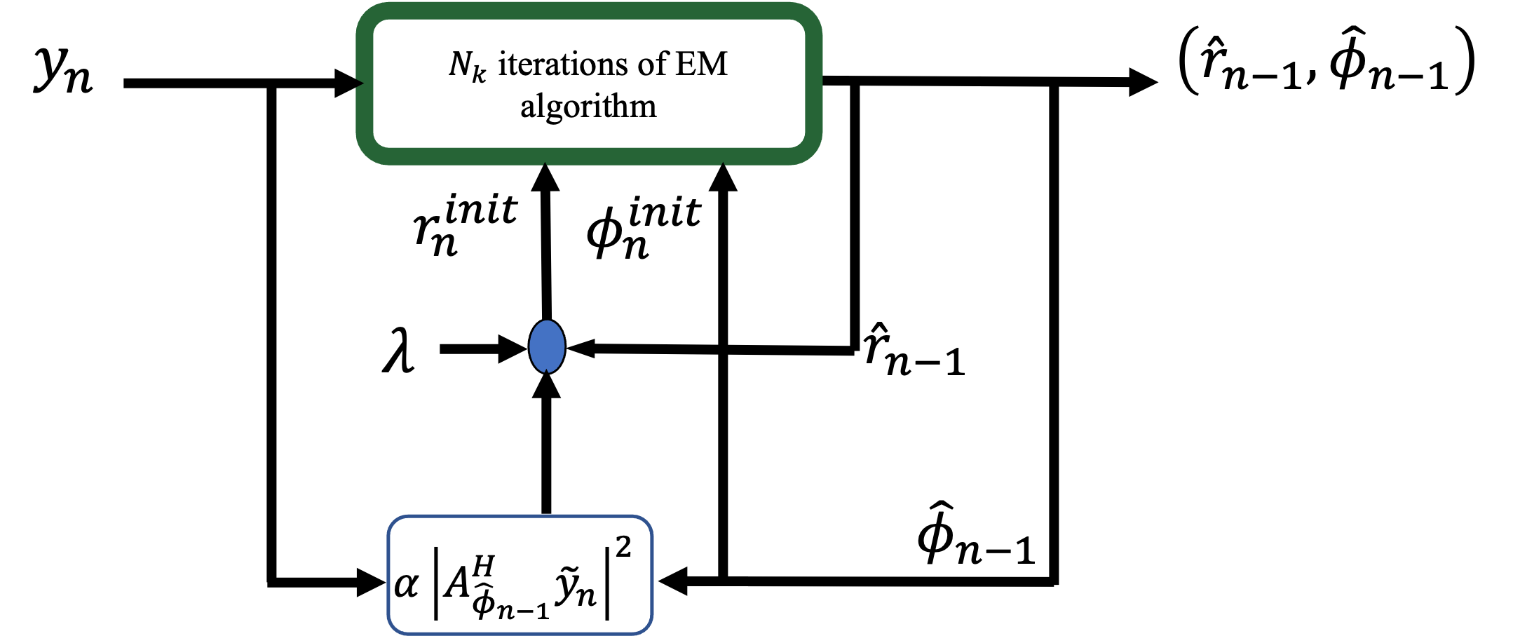
In directed energy applications, must be estimated at a sufficiently high sampling rate, , that the atmospheric phase distortion is nearly unchanged between samples. For this, we propose the Dynamic DH-MBIR (DDH-MBIR) algorithm for estimating and from a streaming sequence of DH data, . Figures 1 and 2 show the pseudo-code and a flow diagram for DDH-MBIR. With each iteration, the data is read, normalized, and then residual tip/tilt removed using least-squares regression. Next, the value of is initialized, and iterations of the EM algorithm are performed.
function DDH_MBIR() ; ; while Data is available do for to do end for WriteData() end while end function
The key innovation of the DDH-MBIR algorithm is the initialization of given by
| (3) |
This initialization leverages the temporal correlation of both and to dramatically reduce the number of EM iterations per time step, (we show later that yields high quality estimates of the phase distortion on simulation data under practical conditions). This initialization is formed by a weighted sum of two terms where and are user selectable weights in the range . Since does not typically change substantially between samples, the first term, , provides a good initial condition for the estimation of .
The second term uses the magnitude squared of the back-projected data. This is typically how images are formed with DH data, and in particular, this is the term that is used in the bootstrapping algorithm of [9]. Intuitively, this second term incorporates a small amount of continuous bootstrapping into the dynamic update loop, which keeps the DDH-MBIR output away from solutions associated with local minima.
Finally, the RemoveTipTilt() function removes the linear component of the phase corresponding to spatial shifts of the reconstructed image; and the Normalize() function is defined as
| (4) |
where is the mean value of and is the number of entries in . This normalization allows algorithmic parameters to be chosen more robustly.
V Experimental Results
In this section, we present estimation results from synthetic data using the Dynamic DH-MBIR algorithm.
V-A Data Simulation
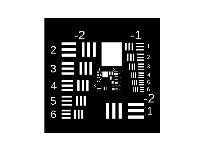
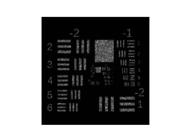
We generated data using the 1951 USAF resolution test chart for along with a frozen flow phase-error model as specified in [10] for . We also removed the piston, tip, and tilt of the phase-errors because we are interested only in estimating the higher-order aberrations. At each timestep, the DH data, , was generated as in [5].
Furthermore, we used an isoplanatic model, image and phase distortion array sizes of where , a sampling frequency of , a Greenwood frequency , a turbulence strength of where is the diameter of the aperture and is Fried’s parameter [11], a wavelength of , and an SNR of .
Using these parameters, we find the magnitude of the phase displacement between time samples by scaling Equation 4.15 in [12] to convert from m/s to pixels/sample. This gives
In our simulation we assumed a flow downward and to the right, which gives a vector displacement of pixels per time step.
V-B Algorithm Parameters and Metrics
In all our simulations, the DDH-MBIR parameters are , , which were found to be the best in a grid search over the range and .
We used peak Strehl ratio, , to evaluate the quality of the phase-errors estimates, where
and is the estimated phase, is back-propagation through a vacuum, and indicates the maximum value of the argument.
V-C Results
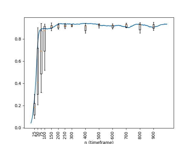
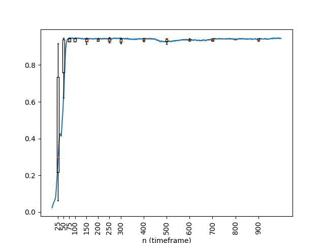
Figures 3 ( or 1 iteration per time step) and 4 () show a box and whiskers plot over 10 simulations, with results from a typical simulation overlaid in blue. In both cases, the Strehl ratio achieves a value within 150 timeframes. However, the case achieves a slightly higher Strehl ratio with less variation at the cost of approximately twice the computation and latency.
The inset in Figure 4 shows the Strehl ratio of a particular simulation versus the time for four different values of . Notice that more iterations per timeframe improves the Strehl ratio but that works well and achieves a Strehl ratio of greater than .
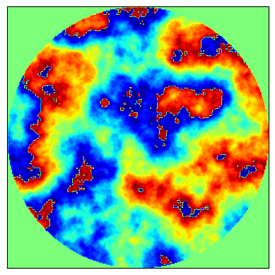
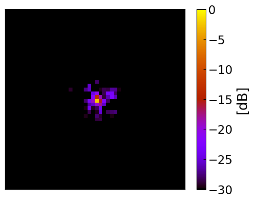
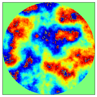
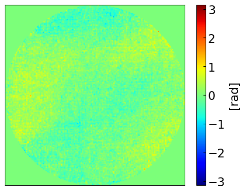
Figure 5 shows the true and estimated phase-errors for time and iterations per timeframe. The residual phase plot is computed by subtracting the true and estimated phase, and the residual PSF is computed by taking the inverse FFT of the residual phase. Both the residual phase and PSF indicate that even with the phase is accurately reconstructed.
VI Conclusion
We described the Dynamic DH-MBIR algorithm for quickly estimating phase-errors due to atmospheric turbulence. Using synthetic DH data generated from frozen flow phase-errors with no boiling, we showed that this algorithm can achieve a Strehl ratio greater than within timeframes using only iteration of the EM algorithm per timeframe. Since the computational cost of each iteration of the Dynamic DH-MBIR algorithm is dominated by two 2D FFTs [8], this makes the Dynamic DH-MBIR algorithm practical for real-time implementation.
References
- [1] J. D. Barchers, D. L. Fried, and D. J. Link, “Evaluation of the performance of hartmann sensors in strong scintillation,” Applied optics, vol. 41, no. 6, pp. 1012–1021, 2002.
- [2] M. F. Spencer, R. A. Raynor, M. T. Banet, and D. K. Marker, “Deep-turbulence wavefront sensing using digital-holographic detection in the off-axis image plane recording geometry,” Optical Engineering, vol. 56, no. 3, p. 031213, 2016. [Online]. Available: https://doi.org/10.1117/1.OE.56.3.031213
- [3] S. T. Thurman and J. R. Fienup, “Phase-error correction in digital holography,” JOSA A, vol. 25, no. 4, pp. 983–994, 2008.
- [4] J. W. Goodman, Speckle Phenomena in Optics, Theory and Applications. Englewood Colorado: Roberts and Company, 2006.
- [5] C. Pellizzari, R. Trahan III, H. Zhou, S. Williams, S. Williams, B. Nemati, M. Shao, and C. A. Bouman, “Optically coherent image formation and denoising using plug and play inversion framework,” JOSA, 2017.
- [6] C. J. Pellizzari, M. F. Spencer, and C. A. Bouman, “Imaging through distributed-volume aberrations using single-shot digital holography,” JOSA A, vol. 36, no. 2, pp. A20–A33, 2019.
- [7] J. D. Schmidt, “Numerical simulation of optical wave propagation with examples in matlab,” in Numerical simulation of optical wave propagation with examples in MATLAB. SPIE Bellingham, WA, 2010.
- [8] V. Sridhar, S. J. Kisner, S. P. Midkiff, and C. A. Bouman, “Fast algorithms for model-based imaging through turbulence,” in Artificial Intelligence and Machine Learning in Defense Applications II, vol. 11543. International Society for Optics and Photonics (SPIE), 2020, p. 118360D.
- [9] C. J. Pellizzari, M. F. Spencer, and C. A. Bouman, “Phase-error estimation and image reconstruction from digital-holography data using a bayesian framework,” JOSA A, vol. 34, no. 9, pp. 1659–1669, 2017.
- [10] S. Srinath, L. A. Poyneer, A. R. Rudy, and S. M. Ammons, “Computationally efficient autoregressive method for generating phase screens with frozen flow and turbulence in optical simulations,” Opt. Express, vol. 23, no. 26, pp. 33 335–33 349, Dec 2015. [Online]. Available: https://opg.optica.org/oe/abstract.cfm?URI=oe-23-26-33335
- [11] D. L. Fried, “Greenwood frequency measurements,” Journal of The Optical Society of America A-optics Image Science and Vision, vol. 7, pp. 946–947, 1990.
- [12] R. K. Tyson, Introduction to Adaptive Optics. SPIE, Mar. 2000. [Online]. Available: https://spiedigitallibrary.org/ebooks/TT/Introduction-to-Adaptive-Optics/eISBN-9780819478603/10.1117/3.358220