11email: hoang.m.pham@campus.tu-berlin.de 11email: sering@math.tu-berlin.de
Dynamic Equilibria in Time-Varying Networks††thanks: Funded by the Deutsche Forschungsgemeinschaft (DFG, German Research Foundation) under Germany’s Excellence Strategy – The Berlin Mathematics Research Center MATH+ (EXC-2046/1, project ID: 390685689).
Abstract
Predicting selfish behavior in public environments by considering Nash equilibria is a central concept of game theory. For the dynamic traffic assignment problem modeled by a flow over time game, in which every particle tries to reach its destination as fast as possible, the dynamic equilibria are called Nash flows over time. So far, this model has only been considered for networks in which each arc is equipped with a constant capacity, limiting the outflow rate, and with a transit time, determining the time it takes for a particle to traverse the arc. However, real-world traffic networks can be affected by temporal changes, for example, caused by construction works or special speed zones during some time period. To model these traffic scenarios appropriately, we extend the flow over time model by time-dependent capacities and time-dependent transit times. Our first main result is the characterization of the structure of Nash flows over time. Similar to the static-network model, the strategies of the particles in dynamic equilibria can be characterized by specific static flows, called thin flows with resetting. The second main result is the existence of Nash flows over time, which we show in a constructive manner by extending a flow over time step by step by these thin flows.
Keywords:
Nash flows over time dynamic equilibria deterministic queuing time-varying networks dynamic traffic assignment.1 Introduction
In the last decade the technological advances in the mobility and communication sector have grown rapidly enabling access to real-time traffic data and autonomous driving vehicles in the foreseeable future. One of the major advantages of self-driving and communicating vehicles is the ability to directly use information about the traffic network including the route-choice of other road users. This holistic view of the network can be used to decrease travel times and distribute the traffic volume more evenly over the network. As users will still expect to travel along a fastest route it is important to incorporate game theoretical aspects when analyzing the dynamic traffic assignment. The results can then be used by network designers to identify bottlenecks beforehand, forecast air pollution in dense urban areas and give feedback on network structures. In order to obtain a better understanding of the complicated interplay between traffic users it is important to develop strong mathematical models which represent as many real-world traffic features as possible. Even though the more realistic models consider a time-component, the network properties are considered to stay constant in most cases. Surely, this is a serious drawback as real road networks often have properties that vary over time. For example, the speed limit in school zones is often reduced during school hours, roads might be completely or partially blocked due to construction work and the direction of reversible lanes can be switched, causing a change in the capacity in both directions. A more exotic, but nonetheless important setting are evacuation scenarios. Consider an inhabited region of low altitude with a high risk of flooding. As soon as there is a flood warning everyone needs to be evacuated to some high-altitude-shelter. But, due to the nature of rising water levels, roads with low altitude will be impassable much sooner than roads of higher altitude. In order to plan an optimal evacuation or simulate a chaotic equilibrium scenario it is essential to use a model with time-varying properties. This research work is dedicated to providing a better understanding of the impact of dynamic road properties on the traffic dynamics in the Nash flow over time model. We will transfer all essential properties of Nash flows over time in static networks to networks with time-varying properties.
1.1 Related Work
The fundamental concept for the model considered in this paper are flows over time or dynamic flows, which were introduced back in 1956 by Ford and Fulkerson [8, 9] in the context of optimization problems. The key idea is to add a time-component to classical network flows, which means that the flow particles need time to travel through the network. In 1959 Gale [10] showed the existence of so called earliest arrival flows, which solve several optimization problems at once, as they maximize the amount of flow reaching the sink at all points in time simultaneously. Further work on these optimal flows is due to Wilkinson [26], Fleischer and Tardos [7], Minieka [18] and many others. For formal definitions and a good overview of optimization problems in flow over time settings we refer to the survey of Skutella [23].
In order to use flows over time for traffic modeling it is important to consider game theoretic aspects. Some pioneer work goes back to Vickrey [24] and Yagar [27]. In the context of classical (static) network flows, equilibria were introduced by Wardrop [25] in 1952. In 2009 Koch and Skutella [15] (see also [16] and Koch’s PhD thesis [14]) started a fruitful research line by introducing dynamic equilibria, also called Nash flows over time, which will be the central concept in this paper. In a Nash flow over time every particle chooses a quickest path from the origin to the destination, anticipating the route choice of all other flow particles. Cominetti et al. showed the existence of Nash flows over time [3, 4] and studied the long term behavior [5]. Macko et al. [17] studied the Braess paradox in this model and Bhaskar et al. [1] and Correa et al. [6] bounded the price of anarchy under certain conditions. In 2018 Sering and Skutella [21] transferred Nash flows over time to a model with multiple sources and multiple sinks and in the following year Sering and Vargas Koch [22] considered Nash flows over time in a model with spillback.
A different equilibrium concept in the same model was considered by Graf et al. [11] by introducing instantaneous dynamic equilibria. In these flows over time the particles do not anticipate the further evolution of the flow, but instead reevaluate their route choice at every node and continue their travel on a current quickest path. In addition to that, there is an active research line on packet routing games. Here, the traffic agents are modeled by atomic packets (vehicles) of a specific size. This is often combined with discrete time steps. Some of the recent work on this topic is due to Cao et al. [2], Harks et al. [12], Peis et al. [19] and Scarsini et al. [20].
1.2 Overview and Contribution
In the base model, which was considered by Koch and Skutella [16] and by the follow up research [1, 3, 4, 5, 6, 17, 21], the network is constant and each arc has a constant capacity and constant transit time. In real-world traffic, however, temporary changes of the infrastructure are omnipresent. In order to represent this, we extend the base model to networks with time-varying capacities (including the network inflow rate) and time-varying transit times.
We start in Section 2 by defining the flow dynamics of the deterministic queuing model with time-varying arc properties and proving some first auxiliary results. In particular, we describe how to turn time-dependent speed limits into time-dependent transit times. In Section 3 we introduce some essential properties, such as the earliest arrival times, which enable us to define Nash flows over time. As in the base model, it is still possible to characterize such a dynamic equilibrium by the underlying static flow. Taking the derivatives of these parametrized static flows provides thin flows with resetting, which are defined in Section 4. We show that the central results of the base model transfer to time-varying networks, and in particular, that the derivatives of every Nash flow over time form a thin flow with resetting. In Section 5 we show the reverse of this statement: Nash flows over time can be constructed by a sequence of thin flows with resetting, which, in the end, proves the existence of dynamic equilibria. We close this section with a detailed example. Finally, in Section 6 we present a conclusion and give a brief outlook on further research directions.
2 Flow Dynamics
We consider a directed graph with a source and a sink such that each node is reachable by . In contrast to the Koch-Skutella model, which we will call base model from now on, this time each arc is equipped with a time-dependent capacity and a time-dependent speed limit , which is inversely proportional to the transit time. We consider a time-dependent network inflow rate denoting the flow rate at which particles enter the network at . We assume that the amount of flow an arc can support is unbounded and that the network inflow is unbounded as well, i.e., for all we require that
Later on, in order to be able to construct Nash flows over time, we will additionally assume that all these functions are right-constant, i.e., for every there exists an such that the function is constant on .
2.0.1 Speed limits.
Let us focus on the transit times first. We have to be careful how to model the transit time changes, since we do not want to lose the following two properties of the base model:
-
(i)
We want to have the first-in-first-out (FIFO) property for arcs, which leads to FIFO property of the network for Nash flows over time [16, Theorem 1].
-
(ii)
Particles should never have the incentive to wait on a node.
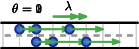
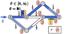
In other words, we cannot simply allow piecewise-constant transit times, since this could lead to the following case: If the transit time of an arc is high at the beginning and gets reduced to a lower value at some later point in time, then particles might overtake other particles on that arc. Thus, particles might arrive earlier at the sink if they wait right in front of the arc until its transit time drops. Hence, we let the speed limit change over time instead. In order to keep the number of parameters of the network as small as possible, we assume that the lengths of all arcs equal and, instead of a transit time, we equip every arc with a time-dependent speed limit . Thus, a particle might traverse the first part of an arc at a different speed than the remaining distance if the maximal speed changes midway; see Figure 1.


2.0.2 Transit times.
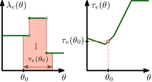
Note that we assume the point queue of an arc to always right in front of the exit. Hence, a particle entering arc at time immediately traverses the arc of length with a time-dependent speed of . The transit time is therefore given by
Since we required to be unbounded for , we always have a finite transit time. For an illustrative example see Figure 3.
The following lemma shows some basic properties of the transit times.
Lemma 1 ().
For all and almost all we have:
-
(i)
The function is strictly increasing.
-
(ii)
The function is continuous and almost everywhere differentiable.
-
(iii)
For almost all we have .
These statement follow by simple computation and some basic Lebesgue integral theorems. The proof can be found in the appendix on page 7.
2.0.3 Speed ratios.
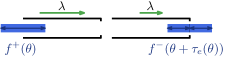
The ratio in Lemma 1 (iii) will be important to measure the outflow of an arc depending on the inflow. We call the speed ratio of and it is defined by . Figuratively speaking, this ratio describes how much the flow rate changes under different speed limits. If, for example, , as depicted in Figure 3, this means that the speed limit was twice as high when the particle entered the arc as it is at the moment the particle enters the queue. In this case the flow rate is halved on its way, since the same amount of flow that entered within one time unit, needs two time units to leave it. With the same intuition the flow rate is increased whenever . Note that in figures of other publications on flows over time the flow rate is often pictured by the width of the flow. But for time-varying networks this is not accurate anymore as the transit speed can vary. Hence, in this paper the flow rates are given by the width of the flow multiplied by the current speed limit.
A flow over time is specified by a family of locally integrable and bounded functions denoting the in- and outflow rates. The cumulative in- and outflows are given by
A flow over time conserves flow on all arcs :
| (1) |
and conserves flow at every node for almost all :
| (2) |
A particle entering an arc at time reaches the head of the arc at time where it lines up at the point queue. Thereby, the queue size at time is defined by .
We call a flow over time in a time-varying network feasible if we have for almost all that
| (3) |
and for almost all .
Note that the outflow rate depends on the speed ratio if the queue is empty (see Figure 3). Otherwise, the particles enter the queue, and therefore, the outflow rate equals the capacity independent of the speed ratio. Furthermore, we observe that every arc with a positive queue always has a positive outflow, since the capacities are required to be strictly positive. And finally, (3) implies (1), which can easily be seen by considering the derivatives of the cumulative flows whenever we have an empty queue, i.e., . By (3) we have that . Hence, (2) and (3) are sufficient for a family of functions to be a feasible flow over time.
The waiting time of a particle that enters the arc at time is defined by
As we required to be unbounded for the set on the right side is never empty. Hence, is well-defined and has a finite value. In addition, is continuous since is always strictly positive. The exit time denotes the time at which the particles that have entered the arc at time finally leave the queue. Hence, we define . In Figure 4 we display an illustrative example for the definition of waiting and exit times.
With these definitions we can show the following lemma.
Lemma 2 ().
For a feasible flow over time it holds for all , and that:
-
(i)
.
-
(ii)
for all .
-
(iii)
.
-
(iv)
For with and we have .
-
(v)
The functions are monotonically increasing.
-
(vi)
The functions and are continuous and almost everywhere differentiable.
-
(vii)
For almost all we have
3 Nash Flows Over Time
In order to define a dynamic equilibrium we consider the particles as players in a dynamic game. For this the set of particles is identified by the non-negative reals denoted by . The flow volume is hereby given by the Lebesgue-measure, which means that with contains a flow volume of . The flow particles enter the network according to the ordering of the reals beginning with particle . It is worth noting that a particle can be split up further so that for example one half takes a different route than the other half. As characterized by Koch and Skutella, a dynamic equilibrium is a feasible flow over time, where almost all particles only use current shortest paths from to . Note that we assume a game with full information. Consequently, all particles know all speed limit and capacity functions in advance and have the ability to perfectly predict the future evolution of the flow over time. Hence, each particle perfectly knows all travel times and can choose its route accordingly. We start by defining the earliest arrival times for a particle .
The earliest arrival time functions map each particle to the earliest time it can possibly reach node . Hence, it is the solution to
| (4) |
Note that for all the earliest arrival time function is non-decreasing, continuous and almost everywhere differentiable. This holds directly for and for it follows inductively, since these properties are preserved by the concatenation and by the minimum of finitely many functions.
For a particle we call an arc active if . The set of all these arcs are denoted by and these are exactly the arcs that form the current shortest paths from to some node . For this reason we call the subgraph the current shortest paths network for particle . Note that is acyclic and that every node is reachable by within this graph. The arcs where particle experiences a waiting time when traveling along shortest paths only are called resetting arcs denoted by .
Nash flows over time in time-varying networks are defined in the exact same way as Cominetti et al. defined them in the base model [3, Definition 1].
Definition 1 (Nash flow over time).
We call a feasible flow over time a Nash flow over time if the following Nash flow condition holds:
| (N) |
where is the set of particles for which arc is active.
As Cominetti et al. showed in [4, Theorem 1] these Nash flows over time can be characterized as follows.
Lemma 3.
A feasible flow over time is a Nash flow over time if, and only if, for all and all we have .
Since the exit and the earliest arrival times have the same properties in time-varying networks as in the base model, this lemma follows with the exact same proof that was given by Cominetti et al. for the base model [4, Theorem 1]. The same is true for the following lemma; see [4, Proposition 2].
Lemma 4.
Given a Nash flow over time the following holds for all particles :
-
(i)
.
-
(ii)
.
-
(iii)
.
4 Thin Flows
Thin flows with resetting, introduced by Koch and Skutella [16], characterize the derivatives and of Nash flows over time in the base model. In the following we will transfer this concept to time-varying networks.
Consider an acyclic network with a source and a sink , such that every node is reachable by . Each arc is equipped with a capacity and a speed ratio . Furthermore, we have a network inflow rate of and an arc set . We obtain the following definition.
Definition 2 (Thin flow with resetting in a time-varying network).
A static - flow of value together with a node labeling is a thin flow with resetting on if:
| (TF1) | |||||
| (TF2) | |||||
| (TF3) | |||||
The derivatives of a Nash flow over time in time-varying networks do indeed form a thin flow with resetting as the following theorem shows.
Theorem 4.1.
For almost all the derivatives and of a Nash flow over time form a thin flow with resetting on in the current shortest paths network with network inflow rate as well as capacities and speed ratios for each arc .
Proof.
Let be a particle such that for all arcs the derivatives of , , and exist and as well as . This is given for almost all .
In order to construct Nash flows over time in time-varying networks, we first have to show that there always exists a thin flow with resetting.
Theorem 4.2 ().
Consider an acyclic graph with source , sink , capacities , speed ratios and a subset of arcs , as well as a network inflow . Furthermore, suppose that every node is reachable from . Then there exists a thin flow with resetting on .
This proof works exactly as the proof for the existence of thin flows in the base model presented by Cominetti et al. [4, Theorem 3]. In addition, a detailed proof utilizing Kakutani’s fixed point theorem is given in the appendix.
5 Constructing Nash Flows Over Time
In the remaining part of this paper we assume that for all the functions and as well as the network inflow rate function are right-constant. In order to show the existence of Nash flows over time in time-varying networks we use the same -extension approach as used by Koch and Skutella in [16] for the base model. The key idea is to start with the empty flow over time and expand it step by step by using a thin flow with resetting.
Given a restricted Nash flow over time on , i.e., a Nash flow over time where only the particles in are considered, we obtain well-defined earliest arrival times for particle . Hence, by Lemma 4 we can determine the current shortest paths network with the resetting arcs , the capacities and speed ratios for all arcs as well as the network inflow rate . By Theorem 4.2 there exists a thin flow on with resetting on . For we set . We extend the - and -functions for some by
and the in- and outflow rate functions by
We call this extended flow over time -extension. Note that means that is empty, and the same holds for .
An -extension is a restricted Nash flow over time, which we will prove later on, as long as the stays within reasonable bounds. Similar to the base model we have to ensure that resetting arcs stay resetting and non-active arcs stay non-active for all particles in . Since the transit times may now vary over time, we have the following conditions for all :
| (5) | ||||
| (6) |
Furthermore, we need to ensure that the capacities of all active arcs and the network inflow rate do not change within the phase:
| (7) | ||||
| (8) | ||||
| Finally, the speed ratios need to stay constant for all active arcs, i.e., | ||||
| (9) | ||||
Lemma 5.
Given a restricted Nash flow over time on then for right-constant capacities and speed limits there always exists a feasible .
Proof.
For the maximal feasible we call the interval a thin flow phase.
Lemma 6 ().
An -extension is a feasible flow over time and the extended -labels coincide with the earliest arrival times, i.e., they satisfy Equation 4 for all .
The final step is to show that an -extension is a restricted Nash flow over time on and that we can continue this process up to .
Theorem 5.1 ().
Given a restricted Nash flow over time on in a time-varying network and a feasible then the -extension is a restricted Nash flow over time on .
Proof.
Finally, we obtain our main result:
Theorem 5.2 ().
There exists a Nash flow over time in every time-varying network with right-constant speed limits, capacities and network inflow rates.
Proof.
The process starts with the empty flow over time, i.e., a restricted Nash flow over time for . We apply Theorem 5.1 with a maximal feasible . If one of the is unbounded we are done. Otherwise, we obtain a sequence , where is a restricted Nash flow over time for , with a strictly increasing sequence . In the case that this sequence has a finite limit, say , we define a restricted Nash flow over time for by using the point-wise limit of the - and -labels, which exists due to monotonicity and boundedness of these functions. Note that there are only finitely many different thin flows, and therefore, the derivatives and are bounded. Then the process can be restarted from this limit point. This so called transfinite induction argument works as follows: Let be the set of all particles for which there exists a restricted Nash flow over time on constructed as described above. The set cannot have a maximal element because the corresponding Nash flow over time could be extended by using Theorem 5.1. But cannot have an upper bound either since the limit of any convergent sequence would be contained in this set. Therefore, there exists an unbounded increasing sequence . As a restricted Nash flow over time on contains a restricted Nash flow over time on we can assume that there exists a sequence of nested restricted Nash flow over time. Hence, we can construct a Nash flow over time on by taking the point-wise limit of the - and -labels, completing the proof. ∎


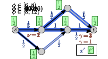


5.0.1 Example.
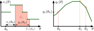
An example of a Nash flow over time in a time-varying network together with the corresponding thin flows is shown in Figure 5 on the next page. On the top: The network properties before time (left side) and after time (right side). In the middle: There are seven thin flow phases. Note that the third and forth phase (both depicted in the same network) are almost identical and only the speed ratio of arc changes, which does not influence the thin flow at all. At the bottom: Some key snapshots in time of the resulting Nash flow over time. The current speed limit is visualized by the length of the green arrow and, for , the reduced capacity is displayed by a red bottle-neck.
As displayed at the top the capacity of arc drops from to at time and, at the same time, the speed limit of arc decreases from to . The first event for particle is due to a change of the speed ratio leading to an increase of . For particle , the top path becomes active and is taken by all following flow as particles on arc are still slowed down. For particle , the speed ratio at arc changes back to but, as this arc is inactive, this does not change anything. Particle is the first to experience the reduced capacity on arc . The corresponding queue of this arc increases until the bottom path becomes active. This happens in two steps: first only the path up to node becomes active for , and finally, the complete path is active from onwards.
6 Conclusion and Open Problems
In this paper, we extended the base model that was introduced by Koch and Skutella, to networks which capacities and speed limits that changes over time. We showed that all central results, namely the existence of dynamic equilibria and their underlying structures in form of thin flow with resetting, can be transfered to this new model. With these new insights it is possible to model more general traffic scenarios in which the network properties are time-dependent. In particular, the flooding evacuation scenario, which was mentioned in the introduction, could not be modeled (not even approximately) in the base model.
There are still a lot of open question concerning time-varying networks. For example, it would be interesting to consider other flows over time in this setting, such as earliest arrival flows or instantaneous dynamic equilibria (see [11]) and show their existence. Can the proof for the bound of the price of anarchy [6] be transfered to this model, or is it possible to construct an example where the price of anarchy is unbounded?
References
- [1] Bhaskar, U., Fleischer, L., Anshelevich, E.: A stackelberg strategy for routing flow over time. Games and Economic Behavior 92, 232–247 (2015)
- [2] Cao, Z., Chen, B., Chen, X., Wang, C.: A network game of dynamic traffic. In: Proc. of the 2017 ACM Conf. on Economics and Comp. pp. 695–696 (2017)
- [3] Cominetti, R., Correa, J., Larré, O.: Existence and uniqueness of equilibria for flows over time. In: Intern. Colloquium on Automata, Languages, and Programming. pp. 552–563. Springer (2011)
- [4] Cominetti, R., Correa, J., Larré, O.: Dynamic equilibria in fluid queueing networks. Operations Research 63(1), 21–34 (2015)
- [5] Cominetti, R., Correa, J., Olver, N.: Long term behavior of dynamic equilibria in fluid queuing networks. In: Integer Programming and Combinatorial Optimization. pp. 161–172. Springer (2017)
- [6] Correa, J., Cristi, A., Oosterwijk, T.: On the price of anarchy for flows over time. In: Proc. of the 2019 ACM Conf. on Economics and Comp. pp. 559–577 (2019)
- [7] Fleischer, L., Tardos, É.: Efficient continuous-time dynamic network flow algorithms. Operations Research Letters 23(3-5), 71–80 (1998)
- [8] Ford, L.R., Fulkerson, D.R.: Constructing maximal dynamic flows from static flows. Operations research 6, 419–433 (1958)
- [9] Ford, L.R., Fulkerson, D.R.: Flows in Networks. Princeton University Press (1962)
- [10] Gale, D.: Transient flows in networks. The Michigan Mathematical Journal 6(1), 59–63 (1959)
- [11] Graf, L., Harks, T., Sering, L.: Dynamic flows with adaptive route choice. Mathematical Programming (2020)
- [12] Harks, T., Peis, B., Schmand, D., Tauer, B., Vargas Koch, L.: Competitive packet routing with priority lists. ACM Transactions on Econo. and Comp. 6(1), 4 (2018)
- [13] Kakutani, S.: A generalization of brouwer’s fixed point theorem. Duke Mathematical Journal 8, 457–459 (1941)
- [14] Koch, R.: Routing Games over Time. Ph.D. thesis, Technische Universität Berlin (2012). https://doi.org/10.14279/depositonce-3347
- [15] Koch, R., Skutella, M.: Nash equilibria and the price of anarchy for flows over time. In: Intern. Symp. on Algorithmic Game Theory. pp. 323–334. Springer (2009)
- [16] Koch, R., Skutella, M.: Nash equilibria and the price of anarchy for flows over time. Theory of Computing Systems 49(1), 71–97 (2011)
- [17] Macko, M., Larson, K., Steskal, L.: Braess’s paradox for flows over time. Theory of Computing Systems 53(1), 86–106 (2013)
- [18] Minieka, E.: Maximal, lexicographic, and dynamic network flows. Operations Research 21(2), 517–527 (1973)
- [19] Peis, B., Tauer, B., Timmermans, V., Vargas Koch, L.: Oligopolistic competitive packet routing. In: 18th Workshop on Algorithmic Approaches for Transportation Modelling, Optimization, and Systems (2018)
- [20] Scarsini, M., Schröder, M., Tomala, T.: Dynamic atomic congestion games with seasonal flows. Operations Research 66(2), 327–339 (2018)
- [21] Sering, L., Skutella, M.: Multi-source multi-sink Nash flows over time. In: 18th Workshop on Algorithmic Approaches for Transportation Modelling, Optimization, and Systems. vol. 65, pp. 12:1–12:20 (2018)
- [22] Sering, L., Vargas Koch, L.: Nash flows over time with spillback. In: Proc. of the Thirtieth Annual ACM-SIAM Symp. on Discrete Algo. pp. 935–945. SIAM (2019)
- [23] Skutella, M.: An introduction to network flows over time. In: Research trends in combinatorial optimization, pp. 451–482. Springer (2009)
- [24] Vickrey, W.S.: Congestion theory and transport investment. The American Economic Review 59(2), 251–260 (1969)
- [25] Wardrop, J.G.: Some theoretical aspects of road traffic research. Proc. of the institution of civil engineers 1(5), 767–768 (1952)
- [26] Wilkinson, W.L.: An algorithm for universal maximal dynamic flows in a network. Operations Research 19(7), 1602–1612 (1971)
- [27] Yagar, S.: Dynamic traffic assignment by individual path minimization and queuing. Transp. Res. 5(3), 179–196 (1971)
7 Appendix: Technical Proofs
See 1
Proof.
-
(i)
Consider two points in time , then is strictly smaller than since
where the strict inequality holds, since is always strictly positive. The last equality follows by the definition of . Hence, with the definition of we have .
-
(ii)
Since is monotone, Lebesgue’s theorem for the differentiability of monotone functions implies that it is almost everywhere differentiable. The same is then true for . The continuity follows directly from the definition since is always strictly positive.
-
(iii)
By the definition of we have
Taking the derivatives of both sides and using Lebesgue’s differentiation theorem together with the chain rule, we obtain
Since is always strictly positive, we get
∎
See 2
Proof.
-
(i)
This follows directly from the definition of the waiting time .
-
(ii)
By equation (3) we have that almost everywhere. Hence, we have by definition that is the minimal value such that
Thus, we obtain for that
Or in short: for . Since is non-decreasing we obtain for all that
- (iii)
-
(iv)
Since we obtain with the monotonicity of together with Lemma 1 (i) that
hence, (3) provides for almost all .
Thus, the definition of implies that equals
Here, we substitute by in order to obtain the first equation. Note that the condition is always satisfied since the right hand side equals and is therefore strictly positive by assumption. Hence, we obtain
-
(v)
Considering two points in time , we show that . Since is non-decreasing, (iii) implies that
(10) If this holds with strict inequality, we obtain by monotonicity of that . If equation (10) holds with equality we have two cases. If , (iv) states that . If , (ii) applied to implies that . Since by Lemma 1 (i) we have , and thus,
-
(vi)
The continuity of follows since is always strictly positive and is continuous, as it is the difference of two continuous functions. Finally, is continuous since it is the sum of three continuous functions.
By (v) the function is non-decreasing for all , and hence, Lebesgue’s theorem for the differentiability of monotone functions states that is almost everywhere differentiable. Since is monotone this also holds for since it is the difference of two almost everywhere differentiable functions. As a sum of almost everywhere differentiable functions, has this property as well.
-
(vii)
The definition of states that
Taking the derivative on both sides we obtain by using the chain rule that
If we have by equation (3) that , and therefore, dividing by (which is strictly positive by assumption) yields
∎
See 4.2
Proof.
Let be the compact, convex and non-empty set of all static --flows of value and let be defined by
where are the node labels associated with uniquely defined by
| (11) |
The existence of a fixed point of is provided by Kakutani’s fixed point theorem [13]
Theorem 7.1 (Kakutani’s Fixed Point Theorem).
Let be a compact, convex and non-empty subset of and , such that for every the image is non-empty and convex. Suppose the set is closed. Then there exists a fixed point of , i.e., .
All conditions are satisfied:
-
•
The set is non-empty, because there has to be at least one path from to with for each arc on . If we set for all arcs on and set every other value to we obtain an element in .
-
•
To see that is convex, note that the arcs that can be used for sending flow, i.e., the ones satisfying , are fixed within the set . Furthermore, every convex combination of two elements only uses arcs that are also used by or .
-
•
In order to show that the function graph is closed let be a sequence within this set, i.e., . Since both sequences, and , are contained in the compact set they both have a limit and within . Let be the sequence of associated node labels of and the node label of . Note that the mapping is continuous, and therefore, it holds that . We prove that . Suppose there is an arc with and . But since is continuous there has to be an such that and for all , which is a contradiction. Hence, is closed.
Since all conditions for Kakutani’s fixed point theorem are satisfied, there has to be a fixed point of . Let be the corresponding node labeling. We show that the pair satisfies the thin flow conditions. Equations TF1 and TF2 follow immediately by (11). For every arc with it holds that since , which shows Equation TF3. Thus, forms a thin flow with resetting, which completes the proof. ∎
See 6
Proof.
Flow conservation on nodes (2) holds since for all we have
Next, we show that the feasibility condition (3) is satisfied. For this we first consider arcs with , which implies . By (TF3) we have that . Since is constant during the thin flow phase, so is , and therefore, we have for all that
In other words, stays active during the thin flow phase.
We consider the outflow rate at time for . In the case of the feasibility condition follows from prior phases. Otherwise, , and therefore,
In the case that we either have , but then there is nothing to show since the interval would be empty, or , which means by (TF2) that either is not active, or it is active but non-resetting. In both cases we have and since for all the queue stays empty during this phase. (3) follows since holds for all . Altogether, we showed that the -extension is indeed a feasible flow over time.
It remains to show that Equation 4 holds, which implies that the extended -functions denote the earliest arrival times. First of all we have
Since is always strictly positive, is the minimal value with this property, which shows (4) for . For we distinguish between three cases for every given arc .
Case 1:
.
Since satisfies (6) it is satisfied for all , and hence,
Case 2:
and .
Since is active we have and (TF2) implies . No
queue builds up as , which means
for all . Combining these yields
Case 3:
since either (if ) or, in the case of , we have
Hence, for all we obtain
This shows that there is no arc with an exit time earlier than the earliest arrival time, and therefore, the left hand side of (4) is always smaller or equal to the right hand side.
It remains to show that the equation holds with equality. For every node there is at least one arc with in the thin flow due to (TF2). No matter if this arc belongs to Case 2 or Case 3 the corresponding equation holds with equality, which shows for all that
This shows that (4) is also satisfied for , which completes the proof. ∎
Lemma 7 (Differentiation rule for a minimum).
For every element of a finite set let be a function that is differentiable almost everywhere and let for all . It holds that is almost everywhere differentiable with
| (12) |
for almost all where .
Proof.
Let such that all , for all , are differentiable, which is almost everywhere. Since all functions are continuous at we have for sufficiently small that for all . It follows that
Note that every point where all are differentiable, but for which the left derivative of does not coincide with the right derivative of , is a proper crossing of at least two functions. Therefore, these points are isolated and form a null set. Hence, we have for almost all . ∎