Dynamic Graph Learning based on Graph Laplacian
Abstract
The purpose of this paper is to infer a global (collective) model of time-varying responses of a set of nodes as a dynamic graph, where the individual time series are respectively observed at each of the nodes. The motivation of this work lies in the search for a connectome model which properly captures brain functionality upon observing activities in different regions of the brain and possibly of individual neurons. We formulate the problem as a quadratic objective functional of observed node signals over short time intervals, subjected to the proper regularization reflecting the graph smoothness and other dynamics involving the underlying graph’s Laplacian, as well as the time evolution smoothness of the underlying graph. The resulting joint optimization is solved by a continuous relaxation and an introduced novel gradient-projection scheme. We apply our algorithm to a real-world dataset comprising recorded activities of individual brain cells. The resulting model is shown to not only be viable but also efficiently computable.
Index Terms:
Dynamic Graph Learning, Graph Signal Processing, Sparse Signal, Convex OptimizationI Introduction
The increased and ubiquitous emergence of graphs is becoming an excellent tool for quantifying interaction between different elements in great variety of network systems. Analyzing and discovering the underlying structure of a graph for a given data set has become central to a variety of different signal processing research problems which may be interpreted as graph structure recovery. For example, in social media [1], such as Facebook and LinkedIn, the basic interaction/relation between two individuals being represented by a link, yields the notion of a graph known as the social network, which is used for inferring further characteristics among all involved individuals [2]. Similarly, in physics [3] and chemistry [4], graphs are widely used to capture the interactions among atoms/molecules to study the behavior of different materials. The rather recent connectome paradigm[5] in neuros-science, is based on the hypothesis that the brain is a massively connected network and its behavior variation and connectivity, particularly in response to controlled external, can be used to investigate brain’s structures and ideally its functionality [6, 7].
Existing analysis approaches of connectivity of neuron signals and associated problems can be categorized into two main groups, Noise correlation analysis[8, 9], which is often applied by neuro- scientists to uncover the connectivity among neurons, Static graph learning [10, 11], which, by way of an optimization procedure, tries to attain a fixed graph over time. Noise correlation is commonly used in neuro-science to establish connectivity between every pair of neurons if their noise correlation over a short time is significant.
This method, however, requires many observations, making it hard to obtain an acceptable connectivity estimation over that interval. Additionally the acquired connectivity does not lend to simple rationalization following an experiment with a specific stimilus.
In the second track, research on estimating graph structures for a given data set has been active and includes graph learning. Research on the latter
has primarily been based on graphs’ topology and signals’ smoothness, and the application of the graph Laplacian has been predominant.
Other recent work includes deep neural network modeling, and the training/testing was performed on graph datasets to ultimately generate a graph to represent patterns under given signals. These studies have primarily focussed on a static graph, with signals non-sparse and the assumption of consistency of the graph over time. These models require sufficiently adequate samples for training and testing, once again making difficult to use on neuronal signals with a typically low sample size, in order to glean the desired variations over small time intervals.
Graphs’ dynamics with clear potential impact on temporal data characterization, have also been of interest by many researchers [12, 13]. In this theme, the models are used to predict the links given previous graphs and associated signals. All these approaches require much prior information on known structures and plenty of data for training and predicting future graphs.
Building on the wealth of prior research work in neuro-science and graph learning [11], we propose a new model, with a dynamic structure goal to track neurons’ dynamic connectivity over time. To that end, our proposed graph will include vertices/nodes for nodes, and their connectivity is reflected by the graph edges whose attribute is determined by the probability/intensity of connection between every pair of neurons.
To proceed, the outline of our paper follows in order our contributions in the sequel. Firstly, exploiting the insight from prior research on graph learning with graph Laplacian [11, 14], we propose an optimization formulation, which can yield a graph over each short time interval which in turn reflects the evolving transformation of the connectivity. Secondly, we modify our model to fit sparse signals so that we can verify our optimized solution on a neuronal signal dataset. Thirdly, we apply three alternative methods to simplify the optimization procedures, to simplify the solution procedures of the optimization problems, and help reach the optimal points. We finally proceed to test our proposed model on a neuronal dataset, to help improve our understanding on the neuronal interaction and their process of transferring signals.
II Problem Setup and Background
For notation clarity and throughout the paper, we will adopt an upper and lower case bold letter to respectively denote a matrix and a vector, and the superscripts to respectively denote its tranpose and inverse. The operator denotes a matrix trace. The identity, zero and ”1” matrices are respectively denoted by
, and , while represents the -th row, -th column element of .
Our neuronal-activity dataset will consist of neuron/nodes, and will be characterized by a connectivity graph , where denotes the vertex set , is the edge set with attributes reflecting the connectivity between each pair of vertices quantified by as a connectivity strength. A time series of observations with , is associated with each node . For simplicity in our derivations, we will aggregate the nodes’ finite length time series into a matrix , where . Our problem formulation will seek for each observed , either a static graph or a time dependent graph series of graphs .
The well known graph Laplacian of an undirected graph can describe its topology, and can serve as the second derivative operator of the underlying graph. The corresponding Laplacian matrix is commonly defined as [15], with , for , adjacent nodes, and otherwise, and where denotes the degree of node . Its simple matrix expression is , where is a diagnal matrix of degrees.
The Laplacian matrix may also usefully adopt, in some context, a second derivative interpretation of graphs: Given an assignment of real number to the nodes, the Laplacian matrix may be found as the second derivative of as ,
where denotes a N-dimensional vector whose elements are all 0s, except the -th element being respectively 1 and -th element -1. As may be seen, represents the first derivative of the edge between the -th and -th node.
The notion of a Laplacian will be exploited in this sequel as a structural regularizer when an optimal graph is sought for a given data set.
III Dynamic Graph Learning
III-A Static Graph Learning
Prior to proposing the dynamic structure learning of a graph, we first recall the principles upon which static graph learning was based [11]. Using the Laplacian quadratic form, , as a smoothness regularizer of the signals , and the degree of connectivity as a tuning parameter, [11] discovers a -sparse graph from noisy signals , by seeking the solution of the following,
| (1) |
where and are tuning parameters, is the noiseless signals and its noisy observation. is the adjacency weight matrix for the undirected graph, with the additional relaxation of the individual weights to the interval .
III-B Dynamic Graph Learning
Note that in [11] a single connectivity graph is inferred for the entire observation time interval, thus overlooking the practically varying connections between every two nodes over time. To account for these variations and towards capturing the true underlying structure of the graph, we propose to learn the dynamics of the graph. Relating these dynamics to the brain signals which are of practical interest, they would not only reflect the signals (as a response to the corresponding stimuli) in that time interval, but also account for their dependence on those in the previous graph and time interval. To that end, we can account for the similarity of temporally adjacent graphs in the overall functionality of the sequence of graphs consistent with the observed data. Selecting a 1-norm distance of connectivity weight matrices between consecutive time intervals, we can proceed with the graph sequence discovery and hence the dynamics by seeking the solution to the following,
| (2) |
where is the penalty coefficient, is the observed data, is the noise-free data, is the weight matrix in the -th time interval, and is a tuning parameter.
III-C Dynamic Graph Learning from Sparse Signals
The solution given by [11] addresses the static graph learning, but the observed signals may often be sparse, which poses a problem: Noting that into the Laplacian quadratic form, we have , calculating the distance between two signals, and we minimize this term to find some nodes with tough connections, in another word, the values of the signals are similar in a small time interval. This equation also implies that if and are close to 0, their distance will also be close to 0. This thus introduces unexpected false edges when sparse signals are present. As a simple illustration, let us assume that sparse signals are rewritten as , where the dimension of is , is an matrix and is . Given that 2-norm is non-negative and the Laplacian matrix is positive semi-definite, we can find a trivial optimal solution of , where is sparse, such that , and the weight matrix can be represented by some block matrix, .
Since problem (3) is a convex and non-negative problem, it can be shown that the optimal loss value is 0 by inserting the solution and into optimization (3). This then shows that if sparse signals (which happens to be the case for brain firing patterns) are present, the solution to the formulated optimization may not be unique , furthermore, yielding some of these optimal points to result in connections between zeros-signal nodes (i.e. meaningless connections per our understanding).
Towards mitigating this difficulty, we introduce a constraint term to help focus on the nodes with significant values, specifically we constrain edge nodes energy to be of significance. This yields the following formulation,
| (3) |
where is a penalty coefficient, and is the -th node signal in the -th time interval. Since the weight matrix for an undirected graph is symmetric, therefore this additional part of the new optimization can be simplified as following:
| (4) |
where is a diagonal matrix defined above from weight matrix . Combining the two expressions from Eqs. (3) and (4) will yield the simpler form of Eq. (6). With a liitle more attention, one could note that this procedure naturally prefers nodes of higher energy by associating a higher weight.
IV Algorithmic Solution
The conventional use of Lagrangian duality for solving the above optimization model is costly in time and memory, and thus begs for an alternative.
IV-A Projection method
To address this difficulty, we consider the constraints as a subspace, where is the whole space for graphs, with , and , such that . Then, we introduce a projection method for projecting the updated into the subspace . Considering an updated weight matrix as a point in a high dimensional space, we minimize the distance between the point and the subspace within the whole space by enforcing
, and .
Applying the Lagrangian Duality on this minimization problem yields,
Claim:
| (5) |
IV-B Proximal operator
In light of the non-smoothness of norm, we call on the proximal operator to solve this part [16]. Firstly, the term in optimization (3) may be affected by the order of updating s. Therefore, to minimize the influence of the order of updating variables, we introduce new variables to replace the this term, and add a new constraint that . Through applying these new variables, updating is not influenced by the others weight matrices, and gives the relaxation between each two adjacent weight matrices. In the end, this would be equivalent to the previous optimization problem, with the advantage of its decreasing the impact on the optimization caused by the order of updating variables.
Claim: As a result, the Lagrangian duality form of the optimization yields the following,
| (6) |
Now we have the function of , denoted as , which is not a smooth but convex function over . To avoid smoothness point, we apply proximal operator to update by projecting the point into the defined convex domain and getting closer to the optimal point. The function is defined as where is some tuning parameter. It is clear that we achieve the optimal point , if and only if we have , therefore for the -th iteration, we update the variable as .
IV-C Algorithm
The function of can be regarded as a convex smooth function, which allows the calculation of the derivative of the optimization formulation over and setting the value to 0.
| (7) |
Since the functions of s are smooth, we use gradient descent to update each . The whole algorithm is presented in Algorithm 1.
V Experiments and results
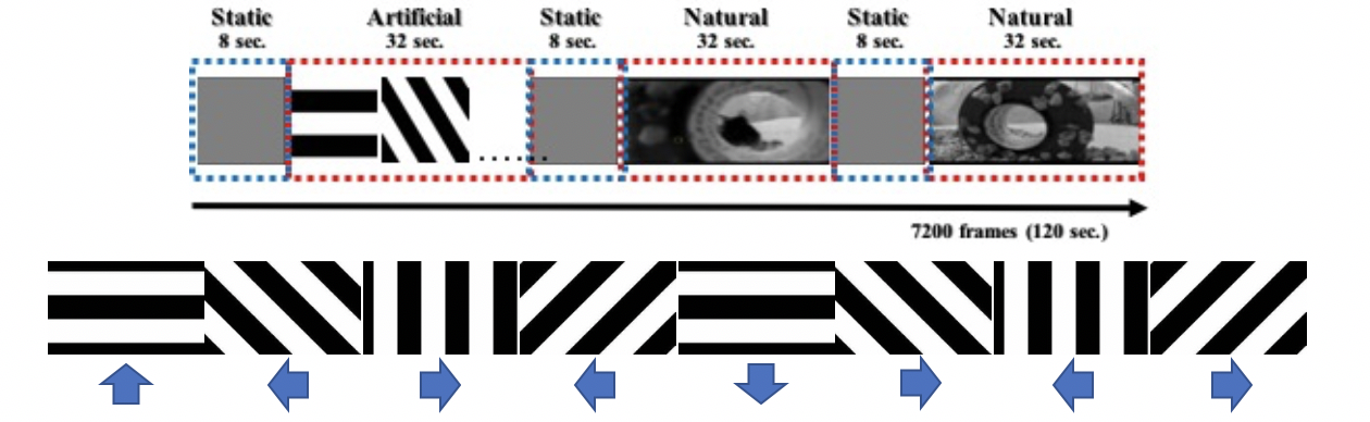
The data in these experiments were measured in S. L. Smith’s Laboratory at UCSB[8]. They use a two-photon electro-microscope [17] to collect fluorescent signals. The whole experiment consists of 3 specific scenarios with a 20 trial measurement, and the stimuli in each trial are the same. The stimuli for each of the scenarios are shown in Figure 1, and consist of ”gray” movie, artificial movie, natural movie 1 and natural movie 2. The dataset includes 590 neurons in V1 area and 301 neurons in AL area, and the sample rate is approximately 13.3 Hz. To select the most consistent 50 neurons in V1 area , We calculate the correlation between signals in every 2 trials for each neuron, and we choose the 50 neurons with the highest mean correlation.
In addition to the similarity under similar stimuli, there is memory across the change of stimuli. The brain’s reaction time for stimuli is 100ms approximately and the delay of the device is around 50 to 100ms, the time difference between 2 time points is 75ms; therefore, we choose in the optimization model to capture the change within 150ms, and we have 25 to 26 graphs for each stimulus. We choose to restrict a sparse graph, 5 percent of number of complete graph. Applying the same parameters on the signals of 20 trials, we have 8 graphs for each trial, where great variations can be observed between different trials. Therefore, we transform the weight matrix to an adjacent matrix through considering the weight matrix as the probability of connectivity between neurons, remove the edges with probability less than 0.5 and set other edges’ weight to 1, then we add the adjacency matrices from different trials in the same time interval, and we choose the value of edges greater than 5.
Through transforming the weight matrix of each graph into a vector and calculating correlation coefficient between every two vectors, e.g. the element value of -th row and -th column of the matrix stands for the correlation between -th and -th graphs’ weight vectors and the matrix is symmetric obviously, the red dash lines divide the plot into small blocks, representing the exact time interval corresponding to each specific stimulus which is shown on the left of the plot, and Fig. 2 gives an intuitive view on the memories between consecutive stimuli and similarities of graphs activated by similar stimuli.
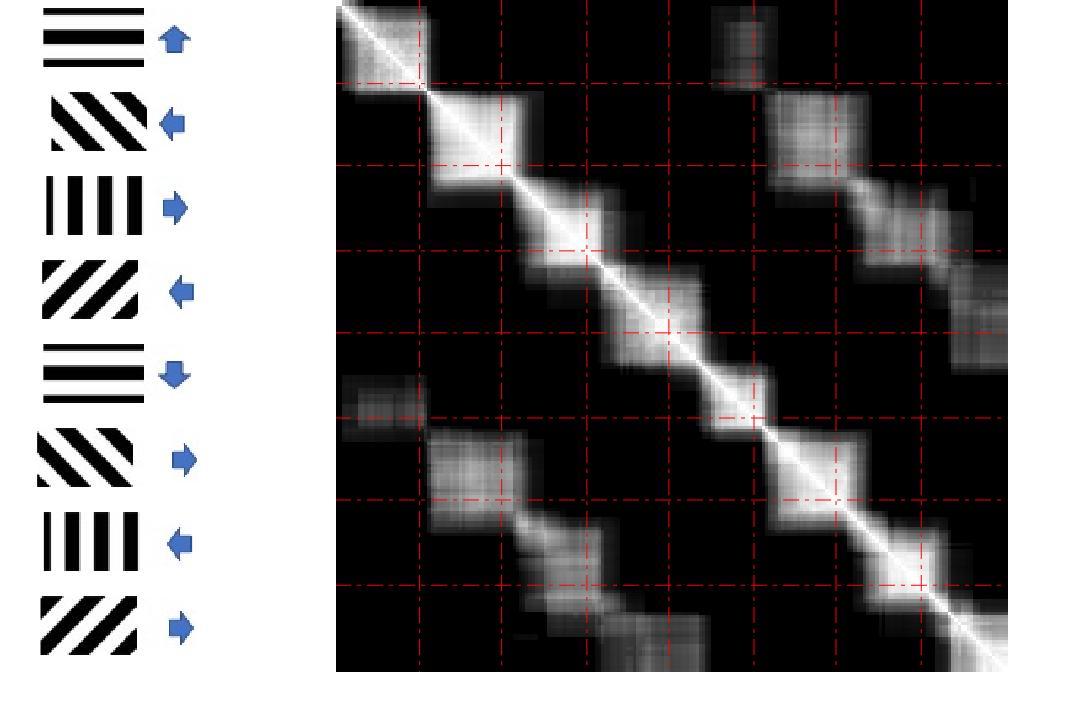
From this neuron signal dataset, we observe variations of neurons’ connectivity over trials, but it preserves similar patterns for similar stimuli in V1 area. Through looking into different time scales, we also show the memorial patterns from one stimulus across to another. These observations can be seen as a basic step for studying brains’ functional connectivity reflecting to the specific stimuli.
VI Conclusion
This paper introduces an optimization model for learning dynamics of sparse graphs with sparse signals based on the graph Laplacian and its smoothness assumption without prior knowledge on the signals. Through applying three alternative solution methods, this model learns a single graph in a short time interval and a set of graphs over the whole signals, and it can capture the small change of graphs in a brief time interval. In the experiment, we solve the difficulty of the low sample rate for detecting graphs, and discover the functional connectivity on specific stimuli instead of revealing the physical connections of neurons. More future research should focus on discovering brains with more datasets and measuring methods, which will support future discovery on understanding how neurons collaborate with each other and how brains work. A future plan is to optimize the model to learn the transformation of graphs.
References
- [1] S. Jagadish and J. Parikh, “Discovery of friends using social network graph properties,” Jun. 3 2014, uS Patent 8,744,976.
- [2] Y. Huang, A. Panahi, H. Krim, and L. Dai, “Fusion of community structures in multiplex networks by label constraints,” in 2018 26th European Signal Processing Conference (EUSIPCO). IEEE, 2018, pp. 887–891.
- [3] G. Audi, A. Wapstra, and C. Thibault, “The ame2003 atomic mass evaluation:(ii). tables, graphs and references,” Nuclear physics A, vol. 729, no. 1, pp. 337–676, 2003.
- [4] A. A. Canutescu, A. A. Shelenkov, and R. L. Dunbrack Jr, “A graph-theory algorithm for rapid protein side-chain prediction,” Protein science, vol. 12, no. 9, pp. 2001–2014, 2003.
- [5] O. Sporns, Discovering the human connectome. MIT press, 2012.
- [6] R. Polanía, W. Paulus, A. Antal, and M. A. Nitsche, “Introducing graph theory to track for neuroplastic alterations in the resting human brain: a transcranial direct current stimulation study,” Neuroimage, vol. 54, no. 3, pp. 2287–2296, 2011.
- [7] G. K. Ocker, Y. Hu, M. A. Buice, B. Doiron, K. Josić, R. Rosenbaum, and E. Shea-Brown, “From the statistics of connectivity to the statistics of spike times in neuronal networks,” Current opinion in neurobiology, vol. 46, pp. 109–119, 2017.
- [8] Y. Yu, J. N. Stirman, C. R. Dorsett, and S. L. Smith, “Mesoscale correlation structure with single cell resolution during visual coding,” bioRxiv, p. 469114, 2018.
- [9] H. Sompolinsky, H. Yoon, K. Kang, and M. Shamir, “Population coding in neuronal systems with correlated noise,” Physical Review E, vol. 64, no. 5, p. 051904, 2001.
- [10] H. P. Maretic, D. Thanou, and P. Frossard, “Graph learning under sparsity priors,” in 2017 IEEE International Conference on Acoustics, Speech and Signal Processing (ICASSP). Ieee, 2017, pp. 6523–6527.
- [11] S. P. Chepuri, S. Liu, G. Leus, and A. O. Hero, “Learning sparse graphs under smoothness prior,” in 2017 IEEE International Conference on Acoustics, Speech and Signal Processing (ICASSP). IEEE, 2017, pp. 6508–6512.
- [12] P. Goyal, S. R. Chhetri, and A. Canedo, “dyngraph2vec: Capturing network dynamics using dynamic graph representation learning,” Knowledge-Based Systems, 2019.
- [13] P. Goyal, N. Kamra, X. He, and Y. Liu, “Dyngem: Deep embedding method for dynamic graphs,” arXiv preprint arXiv:1805.11273, 2018.
- [14] X. Dong, D. Thanou, P. Frossard, and P. Vandergheynst, “Learning laplacian matrix in smooth graph signal representations,” IEEE Transactions on Signal Processing, vol. 64, no. 23, pp. 6160–6173, 2016.
- [15] F. R. Chung and F. C. Graham, Spectral graph theory. American Mathematical Soc., 1997, no. 92.
- [16] N. Parikh, S. Boyd et al., “Proximal algorithms,” Foundations and Trends® in Optimization, vol. 1, no. 3, pp. 127–239, 2014.
- [17] N. Ji, J. Freeman, and S. L. Smith, “Technologies for imaging neural activity in large volumes,” Nature neuroscience, vol. 19, no. 9, p. 1154, 2016.
- [18] S. Boyd and L. Vandenberghe, Convex optimization. Cambridge university press, 2004.
- [19] F. Crick and C. Koch, “Are we aware of neural activity in primary visual cortex?” Nature, vol. 375, no. 6527, p. 121, 1995.
- [20] V. Kalofolias, “How to learn a graph from smooth signals,” in Artificial Intelligence and Statistics, 2016, pp. 920–929.
- [21] D. Wang, P. Cui, and W. Zhu, “Structural deep network embedding,” in Proceedings of the 22nd ACM SIGKDD international conference on Knowledge discovery and data mining. ACM, 2016, pp. 1225–1234.
- [22] S. Cao, W. Lu, and Q. Xu, “Deep neural networks for learning graph representations,” in Thirtieth AAAI Conference on Artificial Intelligence, 2016.
- [23] C. M. Niell and M. P. Stryker, “Modulation of visual responses by behavioral state in mouse visual cortex,” Neuron, vol. 65, no. 4, pp. 472–479, 2010.