Dynamic Sparse Training via Balancing the Exploration-Exploitation Trade-off
Abstract
Over-parameterization of deep neural networks (DNNs) has shown high prediction accuracy for many applications. Although effective, the large number of parameters hinders its popularity on resource-limited devices and has an outsize environmental impact. Sparse training (using a fixed number of nonzero weights in each iteration) could significantly mitigate the training costs by reducing the model size. However, existing sparse training methods mainly use either random-based or greedy-based drop-and-grow strategies, resulting in local minimal and low accuracy. In this work, to assist explainable sparse training, we propose important weights Exploitation and coverage Exploration to characterize Dynamic Sparse Training (DST-EE), and provide quantitative analysis of these two metrics. We further design an acquisition function and provide the theoretical guarantees for the proposed method and clarify its convergence property. Experimental results show that sparse models (up to 98% sparsity) obtained by our proposed method outperform the SOTA sparse training methods on a wide variety of deep learning tasks. On VGG-19 / CIFAR-100, ResNet-50 / CIFAR-10, ResNet-50 / CIFAR-100, our method has even higher accuracy than dense models. On ResNet-50 / ImageNet, the proposed method has up to 8.2% accuracy improvement compared to SOTA sparse training methods.
Index Terms:
Over-parameterization, neural network pruning, sparse trainingI Introduction
Increasing deep neural networks (DNNs) model size has shown superior prediction accuracy in a variety of real-world scenarios [1]. However, as model sizes continue to scale, a large amount of computation and heavy memory requirements prohibit the DNN training on resource-limited devices, as well as being environmentally unfriendly [2, 3, 4, 5, 6, 7]. A Google study showed that GPT-3 [8] (175 billion parameters) consumed 1,287 MWh of electricity during training and produced 552 tons of carbon emissions, equivalent to the emissions of a car for 120 years [9]. Fortunately, sparse training could significantly mitigate the training costs by using a fixed and small number of nonzero weights in each iteration, while preserving the prediction accuracy for downstream tasks.
Two research trends on sparse training have attracted enormous popularity. One is static mask-based method [10, 11, 5], where sparsification starts at initialization before training. Afterward, the sparse mask (a binary tensor corresponding to the weight tensor) is fixed. Such limited flexibility of subnetwork or mask selection leads to sub-optimal subnetworks with poor accuracy. To improve the flexibility, dynamic mask training has been proposed [12, 13, 14], where the sparse mask is periodically updated by drop-and-grow to search for better subnetworks with high accuracy, where in the drop process we deactivate a portion of weights from active states (nonzero) to non-active states (zero), vice versa for the growing process.
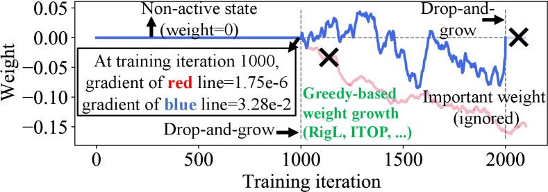
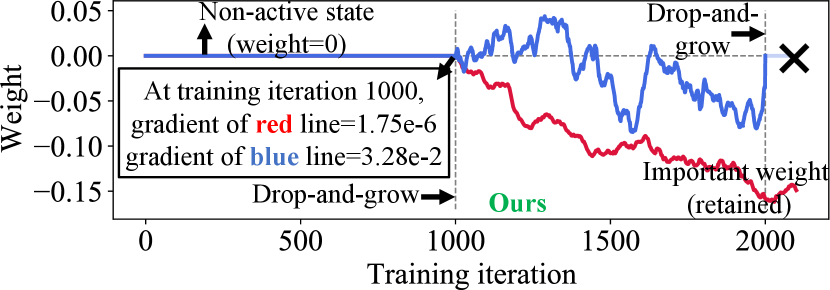
However, these methods mainly use either random-based or greedy-based growth strategies. The former one usually leads to lower accuracy while the latter one greedily searches for sparse masks with a local minimal in a short distance [15], resulting in limited weights coverage and thus a sub-optimal sparse model. As an illustration in Figure 1a using VGG-19/CIFAR-100, at one drop-and-grow stage (1,000th iteration), the gradient-based approach grows non-active weights with relatively large gradients but ignores small gradients. However, as training continues (e.g., at the 2,000th iteration), these non-active weights with small gradients will have large magnitude and hence are important to model accuracy [16, 17]. Therefore, they should be considered for the growth at the 1,000th iteration as shown in Figure 1b. In addition, more than 90% of non-active weights but important weights are ignored in 12 out of 16 convolutional layers.
To better preserve these non-active weights but important weights, we propose a novel weights Exploitation and coverage Exploration characterized Dynamic Sparse Training (DST-EE) to update the sparse mask and search for the “best possible” subnetwork. Different from existing greedy-based methods, which only exploit the current knowledge, we further explore and grow the weights that have never been covered in past training iterations, thus increasing the coverage of weights and avoiding the subnetwork searching process being trapped in a local optimum [18]. The contributions of the paper are summarized as follows:
-
•
To assist explainable sparse training, we propose important weights exploitation and weights coverage exploration to characterize sparse training. We further provide the quantitative analysis of the strategy and show the advantage of the proposed method.
-
•
We design an acquisition function for the growth process. We provide theoretical analysis for the proposed exploitation and exploration method and clarify the convergence property of the proposed sparse training method.
-
•
Our proposed method does not need to train dense models throughout the training process, achieving up to 95% sparsity ratio and even higher accuracy than dense training, with same amount of iterations. Sparse models obtained by the proposed method outperform the SOTA sparse training methods.
On VGG-19 / CIFAR-100, ResNet-50 / CIFAR-10, ResNet-50 / CIFAR-100, our method has even higher accuracy than dense models. On ResNet-50 / ImageNet, the proposed method has up to 8.2% accuracy improvement. On graph neural network (GNN), our method outperforms prune-from-dense using ADMM algorithm [19, 20, 21], achieving up to 23.3% higher link prediction accuracy.
II Related Work
Sparse Evolutionary Training (SET) [12] removed least magnitude valued weights and randomly grow the corresponding number of weights back at the end of each training epoch. SNFS [22] utilized exponentially smoothed momentum to find the important weights and layers, and redistributed pruned weights based on the mean momentum magnitude per layer. RigL [14] updated the sparsity topology of the sparse network during training using the same magnitude-based weights dropping method while growing back the weights using top-k absolute largest gradients, achieving better accuracy than static mask training under same sparsity. However, the greedy-based growth policy leading to limited weights coverage, therefore a sub-optimal sparse model. ITOP [1] discovered that the benefits of dynamic mask training come from its ability to consider across time all possible parameters. In addition, MEST [23] employed a gradually decreasing drop and grow rate with a more relaxed range of parameters for growing. However, both ITOP and MEST keep the same drop-and-growth strategy as the existing works and have limited weights coverage. GaP [24] divides the DNN into several partitions, growing one partition at a time to dense and pruning the previous dense partition to sparse, with the aim of covering all weights. However, it requires more training time than traditional pruning methods, which limits its application on resources limited scenarios.
III Important weights exploitation and coverage exploration
III-A Overview
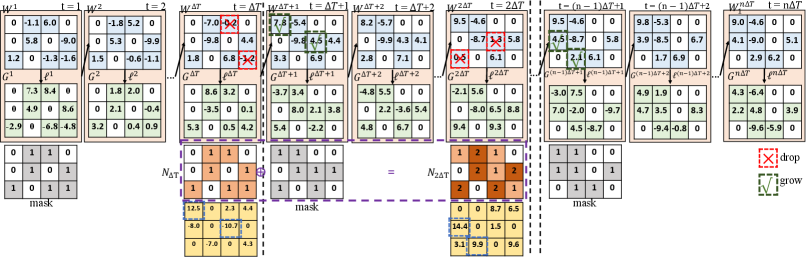
We formalize the sparse training process of the proposed DST-EE as follows. We define a -layer deep neural network with dense weight . During the training process, the weight of -th layer at -th iteration is denoted by . We randomly initialize sparse weight tensor as = with sparsity distribution of using ERK [12] initialization. Each sparse weight tensor within a layer has a corresponding mask tensor (zero elements masked by 0 and other elements masked by 1) with the same size. We define zero elements in weight tensor as non-active weights and others as active weights. For each iteration, we only update the active weights. In addition, every iteration, we update the mask tensor, i.e., for -th layer, we drop the weights that are closest to zero (i.e., smallest positive weights and the largest negative weights), the dropped weights are denoted by ArgTopK. We denote as the counter tensor that collects the occurrence frequency for each 1 mask. We initialize as a zero tensor with the same size as the corresponding weight tensor. Every iteration, the counter tensor is updated by adding the counter tensor with the existing mask tensor. We use to denote the importance score tensor in -th mask update. We design the following acquisition function to compute the importance score tensor
| (1) |
where the first term is the absolute gradient tensor of -th layer at -th iteration. is the loss of -th layer. is the input training data. In the second term , is the coefficient to balance between the two terms and is a positive constant to make the remainder as nonzero. For each importance score tensor, we identify the highest absolute values and select the indices. These corresponding mask values with the same indices will be set to 1s. In the next iteration, we update the weights using the new mask tensor. In the whole process, we maintain that the newly activated weights are the same amount as the previously deactivated weights. We repeat the aforementioned iterations till the end of training. The details of our method are illustrated in Algorithm 1, where means tensor matrix multiplication.
Figure 2 shows the training data flow of one layer using the proposed method. We use and to denote the weight and gradient tensor, respectively. is the total number of rounds of mask updates. is the loss to compute the gradient tensor. In the first iteration of each , the weight tensor has a corresponding binary mask tensor, where zero elements are masked by 0 in the mask tensor and other elements are masked by 1. is the counting tensor, indicating the number of non-zero occurrences in previous mask updates.
III-B Important Weights Exploitation in Sparse Training
In proposed sparse training, we exploit current knowledge (weights and gradients) and define the exploitation score to help decide the mask with the highest accuracy. More specifically, we define the exploitation score in -th mask update as the first item of Eq. (1), i.e., .
We further propose an evaluation metric to quantify the degree of exploitation for weight growth. With high degree of exploitation, the policy will find a model with local minimal with large loss reduction in a short time. Therefore, a growth policy is designed to have a high exploitation degree if it leads to a fast reduction in losses in the next iteration.
To formulate the evaluation metric, we denote as weight of a model, where denotes the weight element in the -th row and -th column of -th layer in the model. -th layer has rows and columns. We further define with same size of . The degree of exploitation is denoted as when the weight element in the -th row and -th column of -th layer is grown in sparse mask update iteration, then
| (2) |
To generalize, we use to denote the degree of exploitation of the model if k weights with indices of are grown, then
| (3) |
III-C Weights Coverage Exploration in Sparse Training
Besides exploitation, we simultaneously choose masks that have never been explored so the model will not be stuck in a bad local optimum. We define our exploration score as the second item in Eq. (1), i.e., , where is a counter tensor that collects the active (nonzero) occurrence frequency of each element. If an element with an active (nonzero) occurrence frequency of zero, it will have a corresponding higher exploration score than explored elements, thus being grown.
Inspired by RigL-ITOP [1], we use an evaluation metric to quantify the degree of exploration for weight growth. Assume is a binary vector to denote if the corresponding parameter in is explored (1) or not (0) throughout the process of sparse training. For exploration rate [1], we use the same formulation as RigL-ITOP [1], i.e., .
III-D Balancing the Exploitation-Exploration Trade-off
The mask tensor search task is challenging in sparse training. Firstly, the mask search task is a high-dimensional problem due to a large number of weights in DNNs. Secondly, the search space has many local minima and saddle points [25, 26] because of the non-convex loss function of DNNs [25, 26]. Therefore, the mask tensor search process is easily trapped in a bad local optimal because of its low global exploration efficiency [18] or needs a longer time to fully explore the loss landscape.
A better balance between exploration and exploitation can encourage search algorithms to better understand the loss landscape and help the sparse model escape from the bad local optima. The importance and challenges of balancing the exploration and exploitation tradeoff have been emphasized in many studies [27, 28]. However, they have not gained enough attention in sparse training. Therefore, there is a strong need to better control the balance and we propose to consider both the exploration and exploitation scores when choosing the mask. And our importance score in Eq. (1) combines the two scores and overcome the limitations of previous work.
| Dataset | #Epochs | CIFAR-10 | CIFAR-100 | ||||
|---|---|---|---|---|---|---|---|
| Sparsity ratio | 90% | 95% | 98% | 90% | 95% | 98% | |
| VGG-19(Dense) | 160 | 93.850.05 | 73.430.08 | ||||
| SNIP [10] | 160 | 93.63 | 93.43 | 92.05 | 72.84 | 71.83 | 58.46 |
| GraSP [11] | 160 | 93.30 | 93.04 | 92.19 | 71.95 | 71.23 | 68.90 |
| SynFlow [29] | 160 | 93.35 | 93.45 | 92.24 | 71.77 | 71.72 | 70.94 |
| STR [30] | 160 | 93.73 | 93.27 | 92.21 | 71.93 | 71.14 | 69.89 |
| SIS [31] | 160 | 93.99 | 93.31 | 93.16 | 72.06 | 71.85 | 71.17 |
| DeepR [32] | 160 | 90.81 | 89.59 | 86.77 | 66.83 | 63.46 | 59.58 |
| SET [12] | 160 | 92.46 | 91.73 | 89.18 | 72.36 | 69.81 | 65.94 |
| RigL [14] | 160 | 93.380.11 | 93.060.09 | 91.980.09 | 73.130.28 | 72.140.15 | 69.820.09 |
| DST-EE (Ours) | 160 | ||||||
| DST-EE (Ours) | 250 | 94.130.09 | 93.670.09 | 92.950.03 | 74.760.07 | 73.910.13 | 71.510.10 |
| ResNet-50(Dense) | 160 | 94.750.01 | 78.230.18 | ||||
| SNIP [10] | 160 | 92.65 | 90.86 | 87.21 | 73.14 | 69.25 | 58.43 |
| GraSP [11] | 160 | 92.47 | 91.32 | 88.77 | 73.28 | 70.29 | 62.12 |
| SynFlow [29] | 160 | 92.49 | 91.22 | 88.82 | 73.37 | 70.37 | 62.17 |
| STR [30] | 160 | 92.59 | 91.35 | 88.75 | 73.45 | 70.45 | 62.34 |
| SIS [31] | 160 | 92.81 | 91.69 | 90.11 | 73.81 | 70.62 | 62.75 |
| RigL [14] | 160 | 94.450.43 | 93.860.25 | 93.260.22 | 76.500.33 | 76.030.34 | 75.060.27 |
| DST-EE (Ours) | 160 | ||||||
| DST-EE (Ours) | 250 | 95.010.16 | 94.920.22 | 94.530.03 | 79.160.06 | 78.660.31 | 76.380.10 |
IV Theoretical Justification
We provide the convergence guarantee for our algorithm. We use to denote the loss function for our sparse training where is the data generation distribution. We use and to denote the complete stochastic and accurate gradients in terms of , respectively. For each round ( iterations), we update the mask and use to denote the mask selected for the q-th round, to denote the model weights after round training. Aligned with [24], we make the following assumptions:
Assumption 1.
(Smoothness). We assume the objective function is partition-wise L-smooth, i.e.,
where is in the same size with .
Assumption 2.
(Gradient noise) We assume for any t and q that
where and is independent of each other.
Assumption 3.
(Mask-incurred error) We assume that
where
Under Assumptions 1-3, we establish Proposition 1 to show that our sparse training algorithm converges to the stationary model at rate under the proper learning rate.
Proposition 1.
If the learning rate , the sparse models generated by our algorithm after Q mask updates will converge as follows:
| (4) | ||||
where is a constant depending on the stochastic gradient noise and the model initialization.
In regard to Proposition 1, we make the following remarks:
Remark 1.
During dense training, we do not have error introduced by the mask and have . As shown in Eq. (4), we will have , indicating that DST-EE will converge to a stationary point as .
Remark 2.
During sparse training, the performance of the model is affected by the error associated with stochastic gradient and introduced by the mask. Our algorithm improves the mask search by a better balance between exploitation and exploration, resulting in a more accurate model.
| Methods | Epochs | Training FLOPS | Inference FLOPS | Top-1 Acc | Training FLOPS | Inference FLOPS | Top-1 Acc |
|---|---|---|---|---|---|---|---|
| ( e18) | ( e9) | (%) | ( e18) | ( e9) | (%) | ||
| Dense | 100 | 3.2 | 8.2 | 76.80.09 | 3.2 | 8.2 | 76.80.09 |
| Sparsity ratio | - | ||||||
| SNIP [10] | - | 0.23 | 0.23 | - | 0.10 | 0.10 | - |
| GraSP [11] | 150 | 0.23 | 0.23 | 72.1 | 0.10 | 0.10 | 68.1 |
| DeepR [32] | - | n/a | n/a | 71.7 | n/a | n/a | 70.2 |
| SNFS [22] | - | n/a | n/a | 73.8 | n/a | n/a | 72.3 |
| DSR [13] | - | 0.40 | 0.40 | 73.3 | 0.30 | 0.30 | 71.6 |
| SET [12] | - | 0.23 | 0.23 | 72.90.39 | 0.10 | 0.10 | 69.60.23 |
| RigL [14] | 100 | 0.23 | 0.23 | 74.60.06 | 0.10 | 0.10 | 72.00.05 |
| MEST [23] | 100 | 0.23 | 0.23 | 75.39 | 0.10 | 0.10 | 72.58 |
| RigL-ITOP [1] | 100 | 0.42 | 0.42 | 75.840.05 | 0.25 | 0.24 | 73.820.08 |
| DST-EE(Ours) | 100 | 0.23 | 0.42 | 76.250.09 | 0.10 | 0.24 | 75.30.06 |
V Experimental Results
V-A Experimental Setup
We evaluate VGG-19 and ResNet-50 on CIFAR-10/CIFAR-100 and evaluate ResNet-50 on ImageNet. The model training and evaluation are performed with CUDA 11.1 on 8 Quadro RTX6000 GPUs and Intel(R) Xeon(R) Gold 6244 @ 3.60GHz CPU. We use a cosine annealing learning rate scheduler with an SGD optimizer. For CIFAR-10/100, we use a batch size of 128 and set the initial learning rate to 0.1. For ImageNet, we use a batch size of 128. We use the same sparsity initialization method ERK in the state-of-the-art sparse training method such as RigL [14] and ITOP [1]. To further validate the generalizability of the proposed method, we conduct experiments on graph neural network for link prediction tasks on ia-email [33] and wiki-talk [34] datasets.
V-B Experimental Results
CIFAR-10/CIFAR-100. The results of CIFAR-10/100 are shown in Table I. We compare our method with SOTA on VGG-19 and ResNet-50 models at sparsity of 90%, 95%, and 98%. To demonstrate the effectiveness of the proposed method, we compare it with three types of methods (i.e., pruning-at-initialization (SNIP, GraSP, SynFlow), dense-to-sparse training (STR, SIS), and dynamic sparse training (DeepR, SET, RigL)) from top to bottom. The results of baselines are obtained from the GraNet [35] paper. Overall, both pruning-at-initialization and dense to sparse methods have higher accuracy than dynamic sparse training (except for RigL (using ITOP [1] setting)). Among the various sparsity ratios, the proposed method achieves the highest accuracy for both VGG-19 and ResNet-50. Using typical training time (total training epochs is 160), there is almost no accuracy loss compared to the dense model at sparsity of 90% on both CIFAR-10 and CIFAR-100. On both VGG-19 and ResNet-50, the proposed method has the highest accuracy compared with SOTA sparse training methods at different sparsity on both CIFAR-10 and CIFAR-10 datasets. For VGG-19, our method has up to 3.3%, 4.6% and 6.7% increase in accuracy on CIFAR-10 and up to 11.1%, 15.3% and 18.8% higher performance in accuracy on CIFAR-100, at sparsity ratios 90%, 95% and 98%, respectively. For ResNet-50, our proposed method has accuracy improvement than RigL with the same training epochs. More specifically, on CIFAR-10, our method has 0.51, 0.86, 0.94 higher accuracy score at sparsity ratio 90%, 95%, 98%, respectively. On CIFAR-100, the accuracy improvements of the proposed method compared to the SOTA sparse training method are 2.2%, 2.0%, 0.83% at sparsity ratios of 90%, 95%, and 98%, respectively.
ImageNet. Table II shows the top-1 accuracy results, training and inference FLOPS on ResNet50 / ImageNet. We use the dense training model as our baseline. For other baselines, we select SNIP [10] and GraSP [11] as the static mask training baselines while adopting DeepR [32], SNFS [22], DSR [13], SET [12], RigL [14], MEST [23], RigL-ITOP [1] as the dynamic mask training baselines as shown in Table II. Compared to static mask training baselines, our proposed method has up to 5.8% and 10.6% increase in accuracy. For the dynamic mask training baselines, RigL is the recently popular baseline, compared with which the proposed method has 2.2% and 3.7% higher Top-1 accuracy at sparsity ratios of 80% and 90%, respectively. For the other two better baselines of sparse training, MEST and RigL-ITOP, our method has 1.1% and 0.5% higher accuracy at a sparsity ratio of 0.8, and 3.7% and 1.48% accuracy improvement at a sparsity ratio of 0.9, respectively.
| Methods | Epochs | Sparsity ratio | Sparsity ratio | Sparsity ratio |
|---|---|---|---|---|
| 80% | 90% | 98% | ||
| Dense | - | 79.72 | ||
| Prune-from-dense | 60 | 79.05 | 78.34 | 78.08 |
| DST-EE (ours) | 50 | 79.28 | 79.13 | 78.58 |
| Methods | Epochs | Sparsity ratio | Sparsity ratio | Sparsity ratio |
|---|---|---|---|---|
| 80% | 90% | 98% | ||
| Dense | - | 83.47 | ||
| Prune-from-dense | 60 | 83.19 | 82.95 | 67.18 |
| DST-EE (ours) | 50 | 83.77 | 83.29 | 82.82 |
Graph Neural Network. Experimental results of sparse training of graph neural network on wiki-talk [34] and ia-email [33] for link prediction task are shown in Table III and Table IV, respectively. We apply the proposed method to the two fully connected layers with uniform sparsity ratios at different sparsity levels, which are 80%, 90%, and 98%. We report the prediction accuracy of the best model searched in 50 training epochs. We compare our method with both the dense model and the best sparse model pruned from the dense model using ADMM algorithm. The prune-from-dense models are trained for 60 epochs in total, which of 20 pretraining epochs, 20 reweighted training epochs, and 20 retraining epochs after pruning. Experimental results show that at a sparsity of 0.8, our sparse training method has even better accuracy than the dense model. The proposed method has accuracy improvement compared with prune-from-dense on both datasets using even fewer training epochs. On wiki-talk [34], our method has 0.29%, 1.0% and 0.64% higher accuracy than prune-from-dense using ADMM algorithm at sparsity ratios of 80%, 90% and 98%, respectively. On ia-email [33], the proposed method has up to 23.3% accuracy improvement than prune-from-dense at a sparsity ratio of 98%.
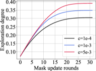
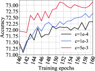
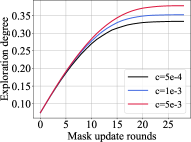
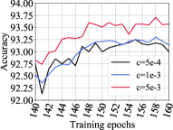
V-C Design Exploration on Different Exploration Degrees.
We investigate the effect of coefficients on exploration degree and test accuracy on VGG-19, CIFAR-10 / CIFAR-100 datasets as shown in Figure 3. The left subfigure in Figure 3a shows the different exploration degree curves generated using different tradeoff coefficients on CIFAR-100 with a sparsity of 0.95. We could see the larger , the higher degree of exploration of the sparse model. The right subfigure in Figure 3a illustrates the test accuracy curves for different coefficients. Within the coefficient range, the larger , the higher test accuracy. The combination of these two subfigures unveils the observation that the higher the exploration degree or higher weights coverage, the higher the test accuracy score. Similar observations are shown in Figure 3b, which validate our methods.
VI Conclusion
In this paper, we propose important weights exploitation and coverage exploration-driven growth strategy to characterize and assist explainable sparse training, update the sparse masks and search for the “best possible” subnetwork. We provide theoretical analysis for the proposed exploitation and exploration method and clarify its convergence property. We further provide the quantitative analysis of the strategy and show the advantage of the proposed method. We design the acquisition function to evaluate the importance of non-active weights for growth and grow the weights with top-k highest importance scores, considering the balance between exploitation and exploration. Extensive experiments on various deep learning tasks on both convolutional neural networks and graph neural networks show the advantage of DST-EE over existing sparse training methods. We conduct experiments to quantitatively analyze the effects of exploration degree. The observations validate the proposed method, i.e., our method could achieve a higher exploration degree and thus a higher test accuracy compared to greedy-based methods.
Acknowledgement
This work was partially funded by the Semiconductor Research Corporation (SRC) Artificial Intelligence Hardware program, and the UIUC HACC program.
References
- [1] Shiwei Liu and et.al. Do we actually need dense over-parameterization? in-time over-parameterization in sparse training. In ICML, pages 6989–7000. PMLR, 2021.
- [2] Shaoyi Huang and et.al. Sparse progressive distillation: Resolving overfitting under pretrain-and-finetune paradigm. In ACL, pages 190–200, 2022.
- [3] Hongwu Peng and et.al. A length adaptive algorithm-hardware co-design of transformer on fpga through sparse attention and dynamic pipelining. In DAC, pages 1135–1140, 2022.
- [4] Panjie Qi and et.al. Accommodating transformer onto fpga: Coupling the balanced model compression and fpga-implementation optimization. In GLSVLSI, 2021.
- [5] Hongwu Peng and et.al. Towards sparsification of graph neural networks. In ICCD. IEEE, 2022.
- [6] Panjie Qi and et.al. Accelerating framework of transformer by hardware design and model compression co-optimization. In ICCAD. IEEE, 2021.
- [7] Daniel Manu and et.al. Co-exploration of graph neural network and network-on-chip design using automl. In Proceedings of the 2021 on Great Lakes Symposium on VLSI, pages 175–180, 2021.
- [8] Tom B. Brown and et.al. Language models are few-shot learners. 2020.
- [9] David Patterson and et.al. Carbon emissions and large neural network training. arXiv preprint arXiv:2104.10350, 2021.
- [10] Namhoon Lee and et.al. Snip: Single-shot network pruning based on connection sensitivity. In ICLR, 2019.
- [11] Chaoqi Wang and et.al. Picking winning tickets before training by preserving gradient flow. ICLR, 2020.
- [12] Decebal Constantin Mocanu and et.al. Scalable training of artificial neural networks with adaptive sparse connectivity inspired by network science. Nature communications, 2018.
- [13] Hesham Mostafa and et.al. Parameter efficient training of deep convolutional neural networks by dynamic sparse reparameterization. In ICML. PMLR, 2019.
- [14] Utku Evci and et.al. Rigging the lottery: Making all tickets winners. In ICML, pages 2943–2952. PMLR, 2020.
- [15] Zheng He and et.al. Sparse double descent: Where network pruning aggravates overfitting. In ICML. PMLR, 2022.
- [16] Alex Renda and et.al. Comparing rewinding and fine-tuning in neural network pruning. arXiv preprint arXiv:2003.02389, 2020.
- [17] Ofir Zafrir and et.al. Prune once for all: Sparse pre-trained language models. arXiv preprint arXiv:2111.05754, 2021.
- [18] Zhiyong Li and et.al. Ps–abc: A hybrid algorithm based on particle swarm and artificial bee colony for high-dimensional optimization problems. Expert Systems with Applications, 2015.
- [19] Hongwu Peng and et.al. Accelerating transformer-based deep learning models on fpgas using column balanced block pruning. In ISQED. IEEE, 2021.
- [20] Shiyang Chen and et.al. Et: re-thinking self-attention for transformer models on gpus. In SC, pages 1–18, 2021.
- [21] Tianyun Zhang and et.al. A systematic dnn weight pruning framework using alternating direction method of multipliers. In ECCV, pages 184–199, 2018.
- [22] Tim Dettmers and et.al. Sparse networks from scratch: Faster training without losing performance. arXiv preprint arXiv:1907.04840, 2019.
- [23] Geng Yuan and et.al. Mest: Accurate and fast memory-economic sparse training framework on the edge. NeurIPS, 34, 2021.
- [24] Xiaolong Ma and et.al. Effective model sparsification by scheduled grow-and-prune methods. In ICLR, 2021.
- [25] Song Han and et.al. Dsd: Dense-sparse-dense training for deep neural networks. arXiv preprint arXiv:1607.04381, 2016.
- [26] Bo Xie and et.al. Diverse neural network learns true target functions. In Artificial Intelligence and Statistics. PMLR, 2017.
- [27] Matej Črepinšek and et.al. Exploration and exploitation in evolutionary algorithms: A survey. CSUR, 2013.
- [28] Robert C Wilson and et.al. Balancing exploration and exploitation with information and randomization. Current opinion in behavioral sciences, 2021.
- [29] Hidenori Tanaka and et.al. Pruning neural networks without any data by iteratively conserving synaptic flow. NeurIPS, 2020.
- [30] Aditya Kusupati and et.al. Soft threshold weight reparameterization for learnable sparsity. In ICML, 2020.
- [31] Sagar Verma and et.al. Sparsifying networks via subdifferential inclusion. In ICML, 2021.
- [32] Guillaume Bellec and et.al. Deep rewiring: Training very sparse deep networks. ICLR, 2018.
- [33] Ryan A. Rossi and Nesreen Ahmed. The network data repository with interactive graph analytics and visualization. In AAAI, 2015.
- [34] Stuart Cunningham and David Craig. Creator governance in social media entertainment. Social Media + Society, 5, 2019.
- [35] Shiwei Liu and et.al. Sparse training via boosting pruning plasticity with neuroregeneration. NeurIPS, 34:9908–9922, 2021.