Dynamical collective memory in fluidized granular materials
Abstract
Recent experiments with rotational diffusion of a probe in a vibrated granular media revealed a rich scenario, ranging from the dilute gas to the dense liquid with cage effects and an unexpected superdiffusive behavior at large times. Here we setup a simulation that reproduces quantitatively the experimental observations and allows us to investigate the properties of the host granular medium, a task not feasible in the experiment. We discover a persistent collective rotational mode which emerges at high density and low granular temperature: a macroscopic fraction of the medium slowly rotates, randomly switching direction after very long times. Such a rotational mode of the host medium is the origin of probe’s superdiffusion. Collective motion is accompanied by a kind of dynamical heterogeneity at intermediate times (in the cage stage) followed by a strong reduction of fluctuations at late times, when superdiffusion sets in.
Introduction - Granular media are systems made of macroscopic particles, shortened “grains”, whose diameter usually exceeds the hundreds of microns, ideally without an upper limit Jaeger et al. (1996); Andreotti et al. (0013). A typical list of granular materials includes sand, powders, cereals, cements, pharmaceuticals, but in certain contexts may incorporate planetary rocks such those in Saturn’s rings Brilliantov et al. (2015). The study of granular media originates from the several applications in chemistry, material sciences and in the management of geophysical hazards. Since several decades, however, it has become a fertile inspiration for theoretical physics, particularly in the framework of non-equilibrium statistical mechanics Pöschel and Brilliantov (2003); Abate and Durian (2008); Ness et al. (2018). In fact, grains can be described as particles which interact dissipatively Brilliantov and Pöschel (2004). Even in dilute conditions and under strong vibro-fluidization, the resemblance between a granular gas and a molecular gas is deceptive, hiding important dynamical differences Puglisi (2015). When packing fraction increases or external energy input decreases, the dissipative nature of granular interactions becomes more and more relevant, making the paradigms of equilibrium statistical physics inapplicable Forterre and Pouliquen (2008).
A state of driven granular matter which has received less attention than others is the liquid one, i.e. a regime of steady agitation, loosely interpreted as “ergodic”, where the spatial arrangement of grains is not a crystal but still shows some degree of order as in molecular liquids Puglisi et al. (2012); Kou et al. (2017). Granular liquids, because of dissipative interactions, display spatial correlations in the velocity field, a property which leads to strong violations of the Fluctuation-Dissipation relation and to interesting memory effects Puglisi et al. (2007); Sarracino et al. (2010a); Gnoli et al. (2014). Another common granular feature is the lack of energy equipartition, for instance in the inhomogeneity of “granular temperature” measured along different directions in an anisotropic setup Feitosa and Menon (2002).
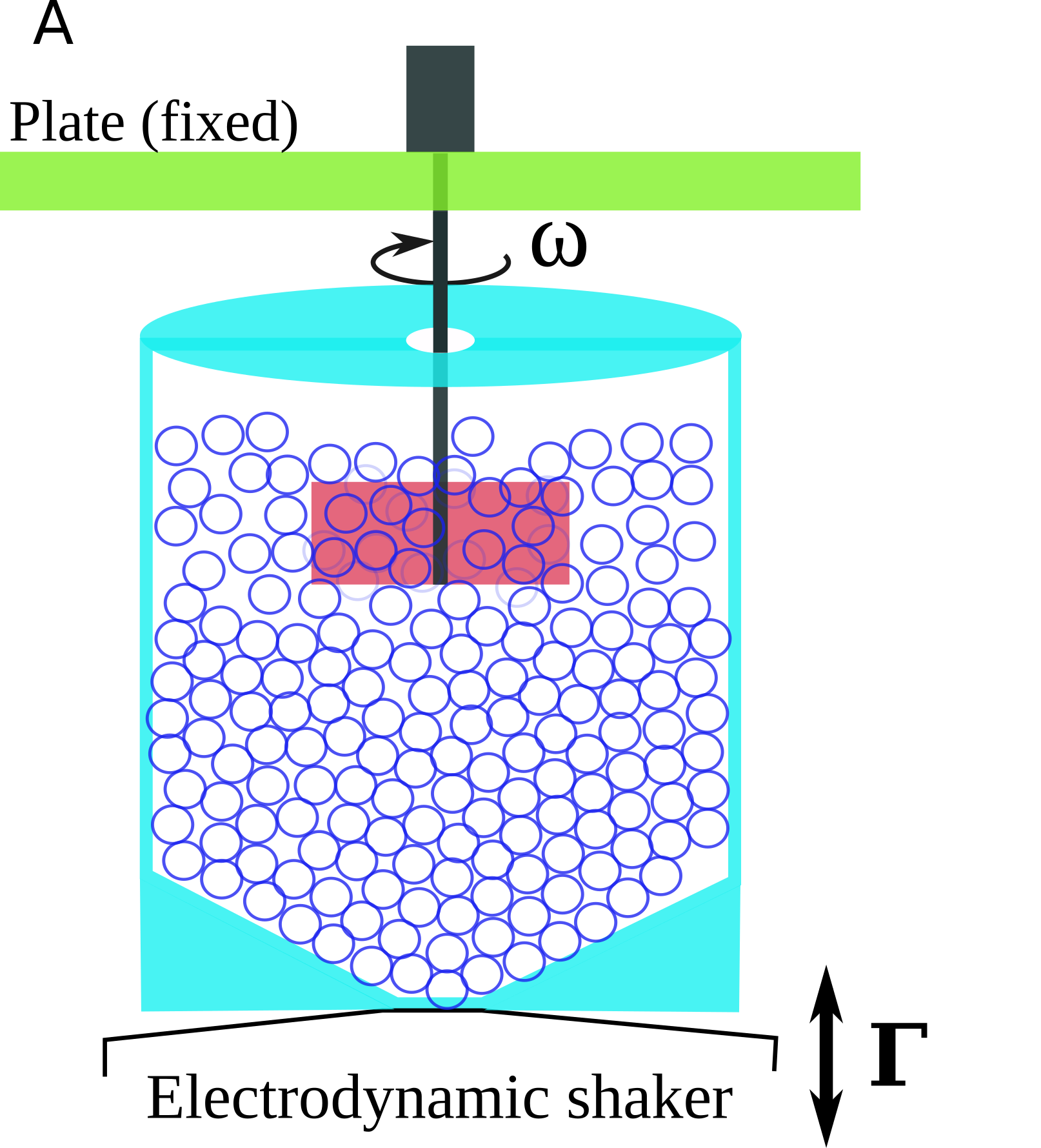
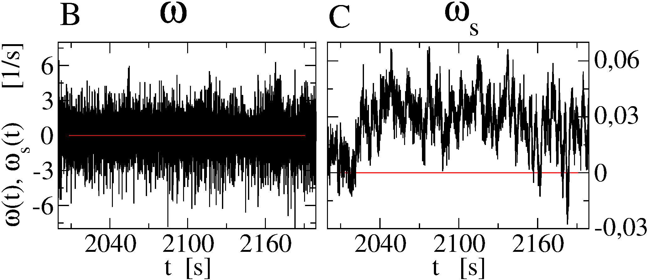
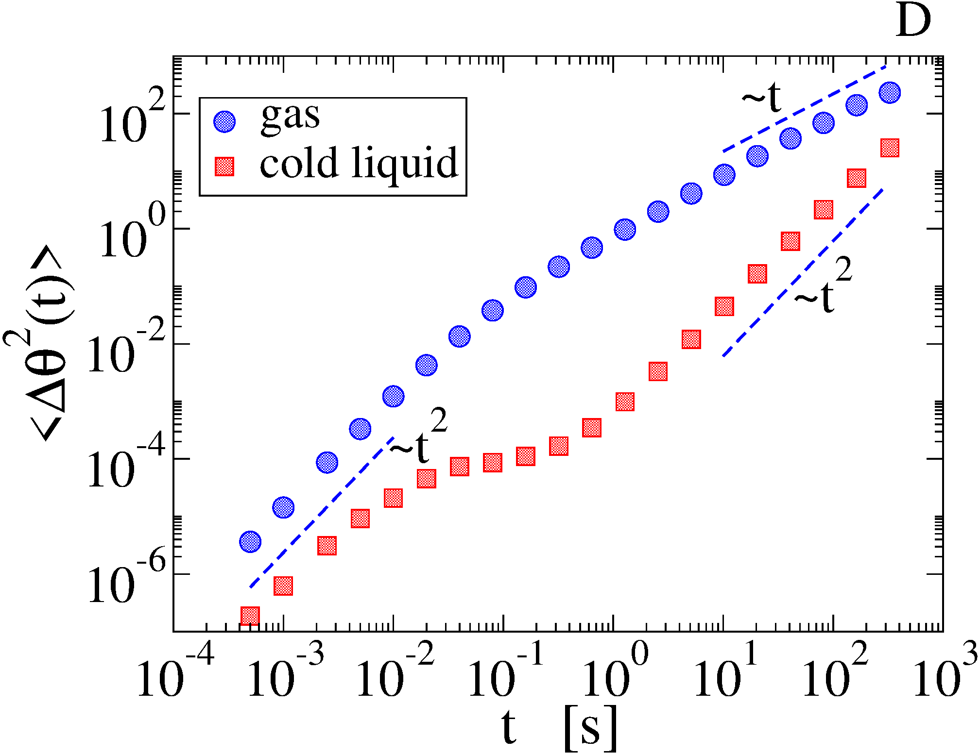
Recently, some of us have conducted a series of experiments with vibrofluidized granular materials, using a blade rotating around a suspended vertical axis as a sort of granular Brownian probe (see Fig. 1A) Scalliet et al. (2015). When the occupied volume fraction is low and vibration is strong, the medium behaves as a gas and the probe displays the typical ballistic-diffusive behavior in the angular mean squared displacement (msd, see Fig. 1D). At high density and weak vibration, the medium becomes a cold liquid and the msd reveals cage effects typical of attempted dynamical arrest. Most importantly, superdiffusion is observed at time delays larger than the onset of the transient cage effect. Filtering out high frequencies of the probe’s angular velocity, one sees a surprisingly long dynamical memory, which may induce quasi-ballistic (angular) flights of the probe for times of the order of tens of seconds (see 1B and 1C). Up to now only phenomenological models have caught this behavior Lasanta and Puglisi (2015), leaving unexplored its microscopic origin, which certainly resides in an unconventional dynamics of the granular host medium. Indeed, a crucial element of those simplified models is an emergent, effective, giant momentum of inertia of the probe, which may compare with that of the whole granular system. Analogies may be found in recent experimental works, where persistent collective motion Briand et al. (2018); Kou et al. (2018) or anomalous diffusion Kou et al. (2017) have been observed in vibrofluidized granular materials made of anisotropic particles, a crucial difference with the work discussed here. In this Letter we reproduce the experimental observations for the probe through a 3D discrete-elements model of the real setup including grains’ rotations and dissipation through normal and tangential interactions. After having shown the quantitative agreement between simulations and the experiment, we focus on the granular medium alone. Our results give direct evidence of a collective dynamical memory, originated in a kind of synchronization between grains movements over long time-scales.
Experimental and numerical setup. The experiment, realized in Scalliet et al. (2015), is sketched in Fig. 1A. Here we report the results of a numerical simulation which is meant to reproduce the setup (container, grains and rotator) in its spatial and temporal proportions. Both the real and the simulated systems consist of a cylinder-shaped recipient (diameter 90 mm, maximum height 47 mm and total volume 245 ), with an inverse-conical-shaped base, containing a number of steel spheres (diameter mm, mass g), representing the “granular medium”. The recipient is vertically vibrated: the real system was mounted on an electrodynamic shaker fed with a noisy signal (spectrum approximately flat in the range Hz and roughly empty outside that range), in the simulated system instead the container is vibrated with a sinusoidal law for its top vertical position , with a constant frequency Hz and amplitude mm. We recall that the maximum vertical acceleration (divided by gravity ) varies in the range and the maximum vertical velocity in mm/s. The effect of the shaking is the fluidization of the granular medium, which - depending on and - stays in a steady gas or liquid regime. The probe for diffusion is a blade (dimensions mm, momentum of inertia g mm2) mechanically isolated from the container, that can rotate around a centered vertical axis and takes energy only from collisions with the granular medium. The angular velocity of the blade and its absolute angle of rotation are measured in the experiment by an encoder with high spatial and temporal resolution (see Supplemental Materials in Scalliet et al. (2015)). The numerical simulations are performed with a discrete-elements model implemented by LAMMPS package Plimpton (1995) with interactions obeying a nonlinear visco-elastic Hertzian model that takes into account the relative deformation of the grains. In order to properly reproduce the soft collision dynamics, simulations run with a time step of s. Our macroscopic phenomena occur on time-scales larger than s, therefore we integrate the dynamics for total times s, spanning more than eight decades of time-steps. More details about the simulation, including the parameters that control the dissipative and the elastic contributions of the interaction, are given in the Supplemental Material (SM) sm . There the reader can also find a table with the correspondence between and best estimates of the packing fraction . We stress that, in view of the collective nature of the phenomena studied here, it is reasonable to expect a certain robustness of the results with respect to the microscopic details. Indeed, the main experimental phenomena are qualitatively reproduced in large regions of the parameters’ space. The effects of changing the dissipation of interactions, the mass or the diameter of particles are discussed in the SM sm . Here we focus on the particular set of values exhibiting the optimal quantitative agreement (within a tolerance of roughly ) with the experiment.
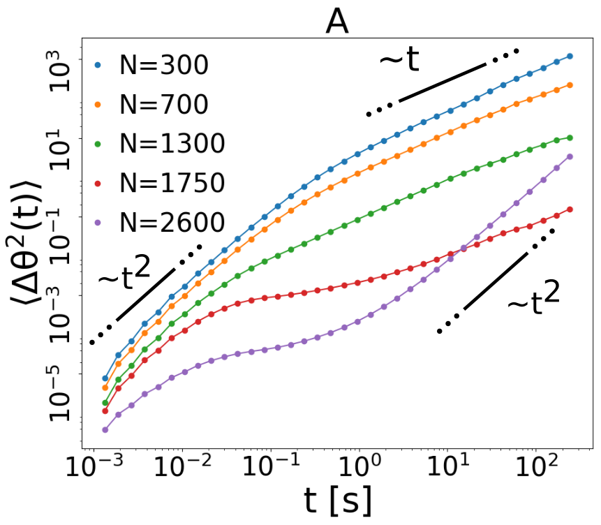
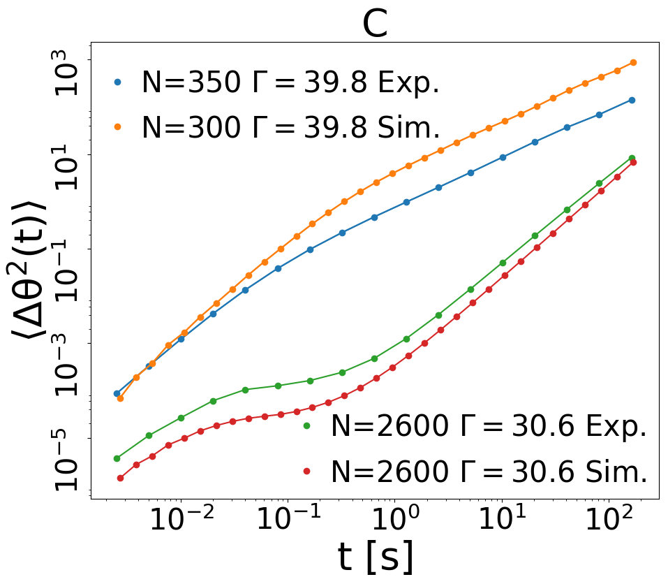
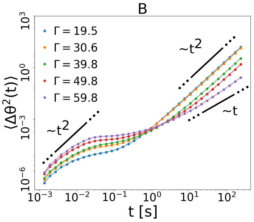
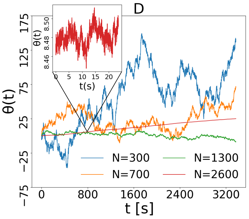
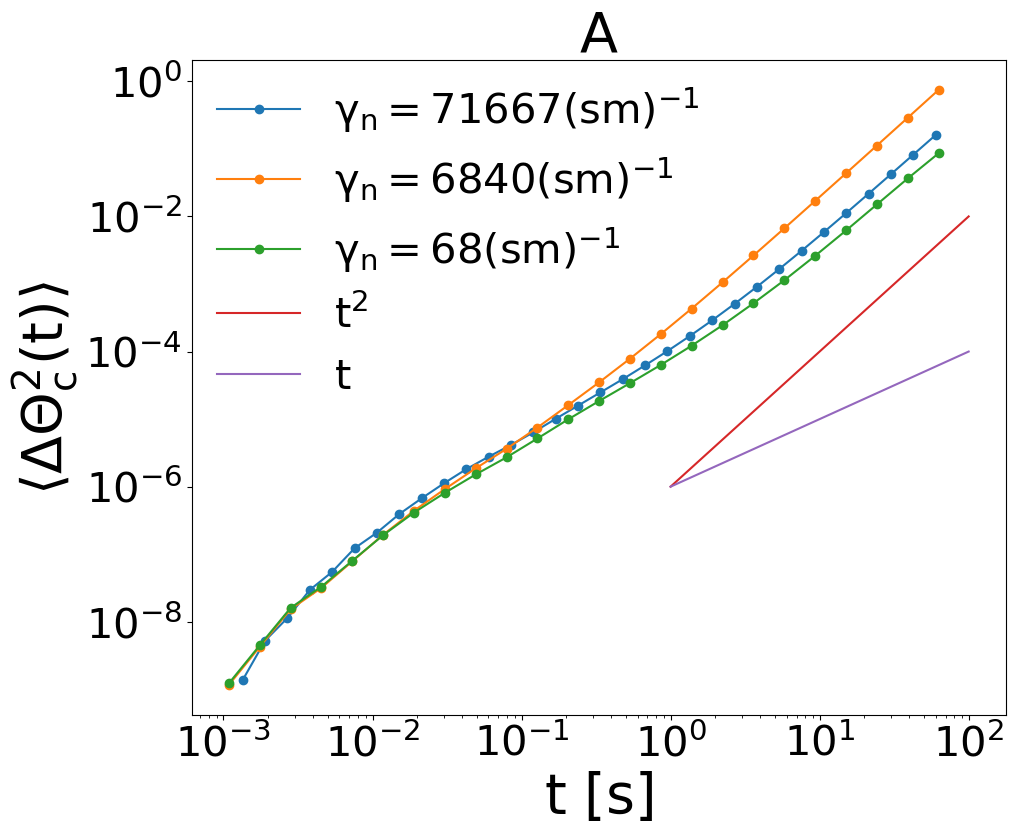
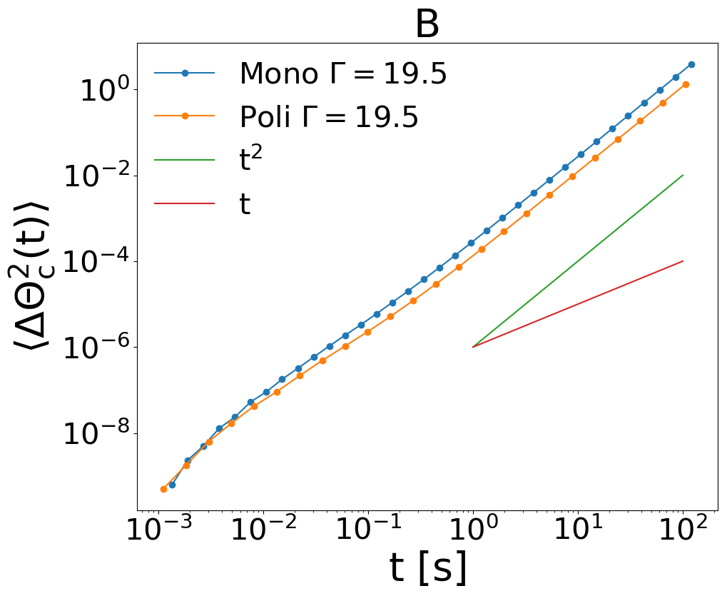
Numerical results: study of the probe. We first compare numerical and experimental results for velocity fluctuations (proportional to probe’s kinetic temperature), not shown here, which fairly agree in the whole range of values of and . In Fig. 2 A and B we show the results of the crucial test of our simulation, i.e. the msd in many different situations. When is small and is high (cyan, yellow and green curves in frame A) the granular medium provides the blade with uncorrelated impacts and the large mass of the probe is sufficient to predict a leading order Ornstein-Uhlenbeck behavior Sarracino et al. (2010b); Gnoli et al. (2013): this determines the typical ballistic () to diffusive () scenario. When increases the medium entraps the probe - similarly to the cage effect in molecular liquids - resulting in a transient arrest of the msd at intermediate times , followed by the usual “escape” with the behavior when (red curve in frame A, purple curve in frame B). A peculiar granular feature is the possibility to develop late-time superdiffusive behavior, when is increased further (purple curve in frame A) or reduced further (cyan, yellow, green and red curves in frame B). At the smallest values of we observe the limit case when . In Fig. 2C we demonstrate the good comparison, appreciable also at the quantitative level, between the msd observed in the simulations and in the experiments, in two very different cases. Finally, in Fig. 2D we show some examples of the numerical time-series (along hour) when is tuned from the dilute gas to the dense liquid (constant ). This plot reveals the significant change in the probe’s dynamics induced by the variation of surrounding granular density. We remind that dissipative interactions naturally reduce velocity fluctuations when is raised at constant . Besides this, a non-trivial memory effect clearly emerges, with long relaxation times evident in the persistence of the direction of motion.
Numerical results: study of the medium. Once the simulation has been successfully compared with the experimental results, we can obtain new information which was unreachable experimentally, due to the 3D nature of the setup. Our first focus is on the most natural collective variables which could be coupled to the angular velocity of the blade, that is the average angular velocity of the granular medium (with respect to the central axis)
| (1a) | ||||
| (1b) | ||||
and its time-integral which represents a collective absolute angle .
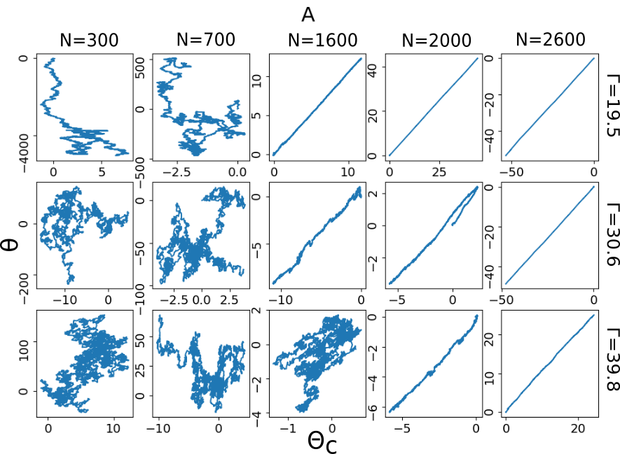
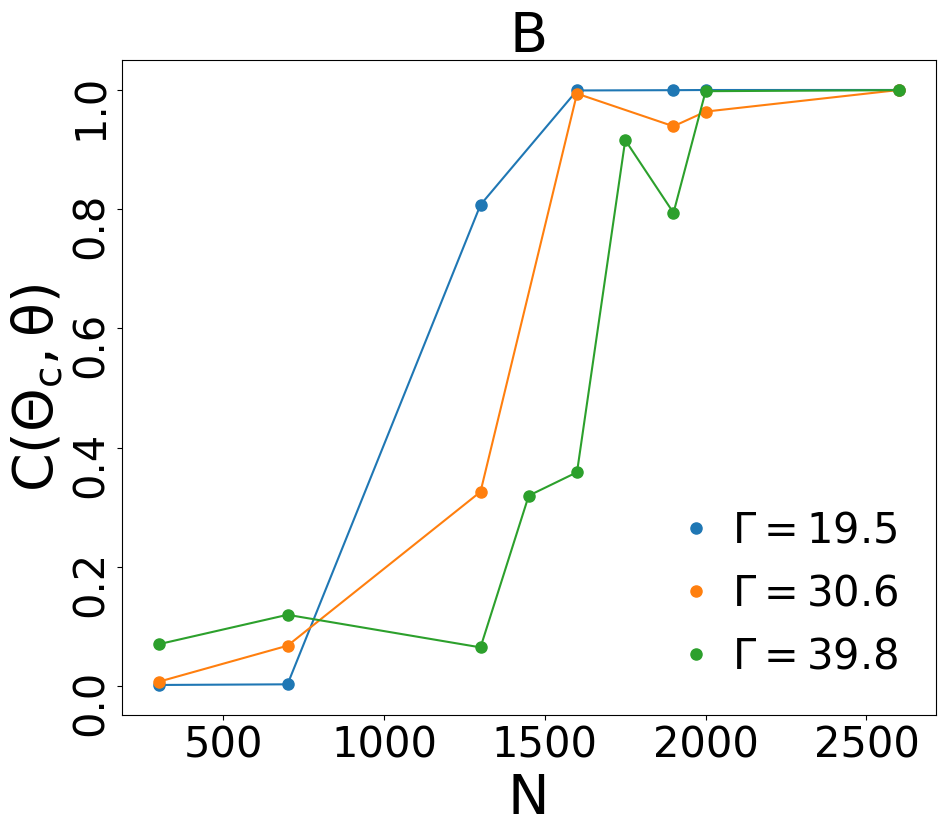
A solid evidence that is meaningful with respect to the anomalous diffusive properties of the probe can be found in Fig. 3. Frame A reports the parametric plot (blade’s angle) vs. (collective angle). It is immediately clear that a sort of crossover line exists in the plane of parameters (with, in fact, a weak dependence on coordinate): for small values of and high values of one has a phase where and are mostly uncorrelated. On the contrary, for large and small a strong correlation emerges between the two signals. In Fig. 3B we show a covariance defined as
| (2) |
with , and the average runs over data sampled for the whole simulation time (typical simulation times are 3600 s with a temporal step s). Note that this estimator of the covariance can also be rewritten as . Frame B of Fig. 3 confirms that it can be interpreted as an order parameter distinguishing between those two phases, and that the crossover occurs, with a fair sharpness, at a value only weakly dependent upon .
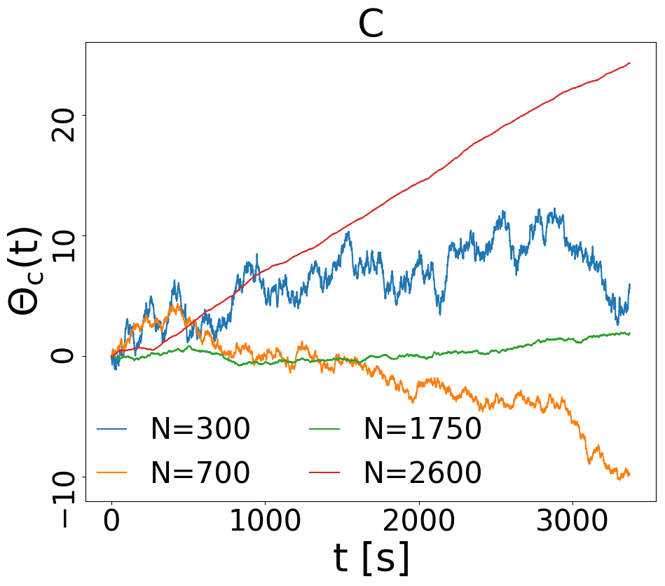
The results of the previous analysis make clear that in the dense/cold cases, when seen from the point of view of large time-scales (, roughly speaking), the dynamics of the blade is strongly correlated to the collective rotation of the granular medium, which is the real hallmark of the transition. This suggests us to focus on a new series of simulations without the rotating blade, with the aim of focusing upon the granular medium itself 111Our analysis revealed that the behavior of the granular medium is largely independent from the presence or absence of the blade, however a blade-free simulation seemed us cleaner with respect to assessing the minimal ingredients of the observed dynamics.. The analysis of in these “blade-free” simulations, shown in a few relevant cases in Fig. 3C, immediately corroborates this intuition: the collective absolute angle of the granular medium is erratic and Brownian-like for and much more smooth at . In particular the cases at appear constituted by long periods where travels in a constant direction, interrupted by rare turns. The average time between those turns seem to increase with , up to a point (case at the largest available , red curve) where it is longer than the whole simulation. We also run longer simulations, not shown here, confirming that sudden turns occur also at , but with seconds. The interesting connection between spatial rearrangements and changes of rotation speed or direction has eluded our attempts and remains an open question for future investigations.
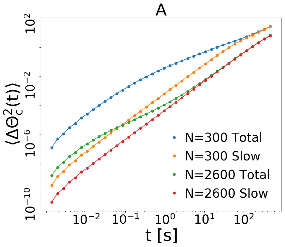
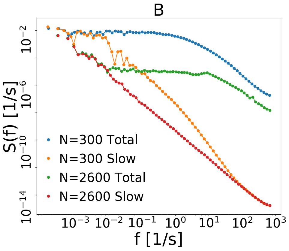
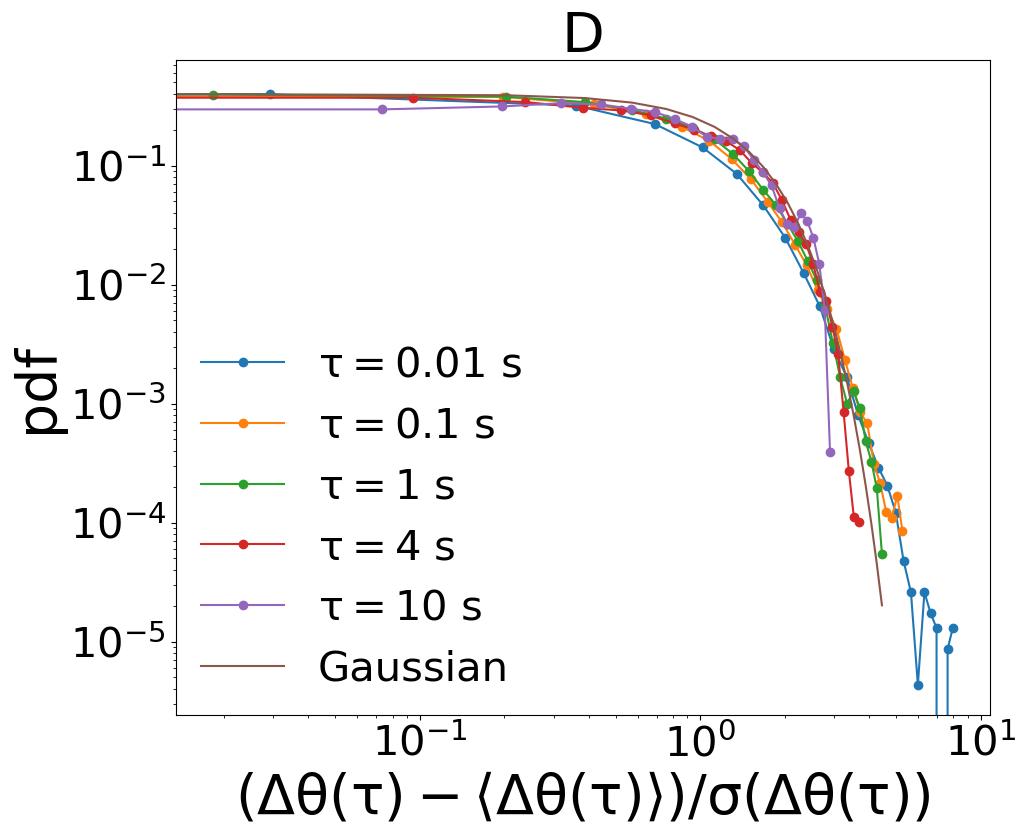
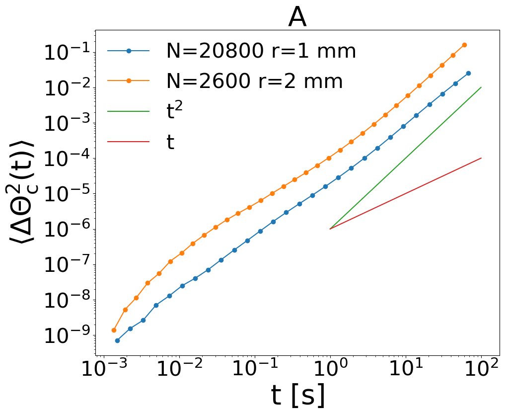
As expected from the strong correlation between and , for , the large-time behavior of the msd of is superdiffusive exactly as already seen for the probe, see Fig. 4A. We have also verified, see SM sm , that the distributions of angular displacements at times larger than are always close to Gaussian, ruling out large tails such as those in Lechenault et al. (2010). Superdiffusive behavior is therefore caused by the long persistent angular drifts discussed before. The connection is the following: in the dense cases becomes huge; therefore what we call “large times”, with respect to microscopic and intermediate () timescales, are actually “small times” with respect to . Only following the signal for times much longer than one would recover the asymptotic (or “final”) diffusive behavior . In order to focus on the dynamics at time-scales , we get rid of the smaller time-scale by defining the slow collective velocity , with larger than (for instance s). Defining, analogously, the slow component of , i.e. gives also the possibility of looking at the collective msd when the fast position oscillations are filtered out, see again Fig. 4A. The slow component, surprisingly, has always a persistent ballistic-like motion, even in the most dilute cases. However, in the dilute cases this ballistic motion is a very weak signal and does not appear in the msd of the total variable. The same observation can be seen for the power spectrum of the angular velocity which is defined as Scalliet et al. (2015), shown in Fig. 4B. In both dilute and dense cases the slow component (yellow and red curves) has a Lorentzian-shaped spectrum, with a flat part at small frequencies and a decaying part, roughly at larger frequencies. Only in the dense case such a low-frequency “flat” part intervenes at very small frequencies, so that part of emerges in the total signal. We verified that changing around a value slightly larger than does not affect this scenario.
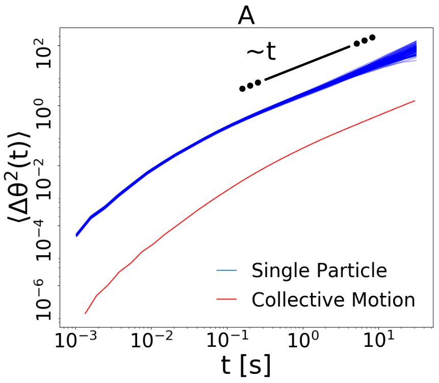
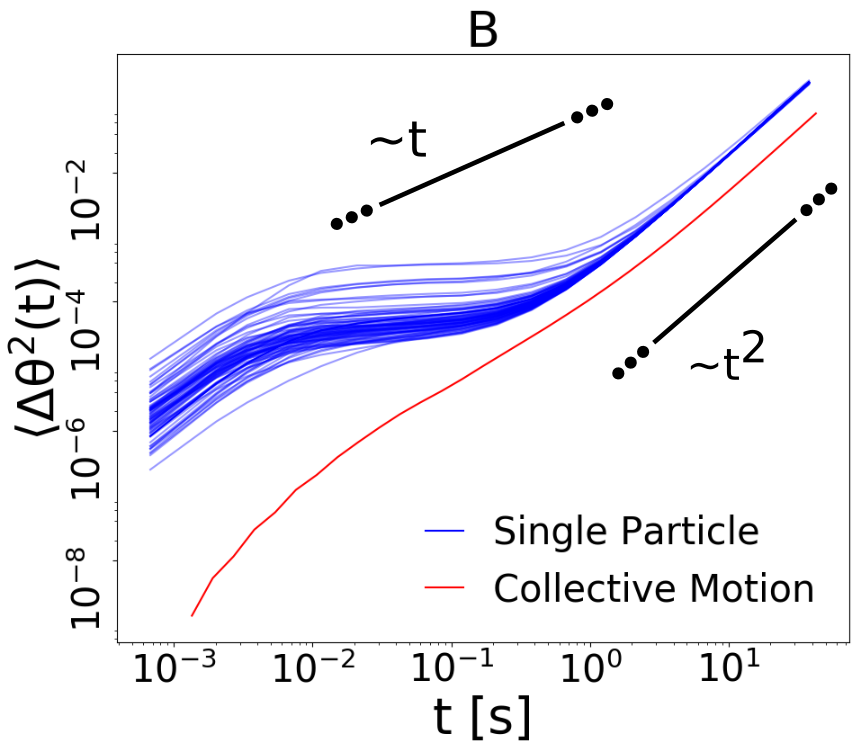
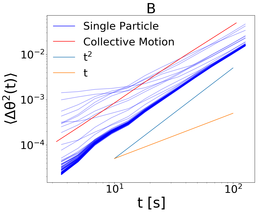
A last question which we address concerns fluctuations, which may be crucial to define a proper correlation length. In glassy systems a well established route is to study dynamical heterogeneities, i.e. wide variations in the local mobility of the medium between different samples Ediger (2000); Berthier et al. (2011); Dauchot et al. (2005); Keys et al. (2007); Candelier et al. (2009). A first encouraging information comes by analyzing the difference in the msd of particles randomly picked, uniformly in space, in the whole system. Fig. 5 indicates that the dense case, with respect to the dilute one, exhibits a much wider volatility of msd. Such heterogeneity is large at intermediate times and rapidly decreases at late times, i.e. when superdiffusion sets in. This confirms that superdiffusion is related to a strong coordination in the trajectories of particles.
In conclusion, we demonstrate that probe’s anomalous diffusion originates in a collective mode of the host granular medium, even if it is constituted of many non-polar particles. The slow component of the grains’ movement along a direction which is free of obstacles, i.e. rotation around the central axis, is more and more coordinated and persistent as density increases and temperature decreases. The observed strong and enduring correlations are not particularly sensitive to changes in the dissipation and in the size of the system and, noticeably, to the degree of configurational (e.g. crystalline) order, see SM sm . The robustness of our results suggests that they could apply to other systems, for instance granular materials under different conditions of fluidizations, as well as disordered glassy systems and fluids of active particles. The dynamical memory displayed by our system could be a more easy to observe proxy for very slow configurational relaxation in hard sphere glasses G. Gradenigo and Puglisi (2010). Moreover, persistent alignment of velocities of inertial active particles is observed in animal collective behavior, such as in flocks Cavagna et al. (2018). While its theoretical connection with granular materials is established Manacorda and Puglisi (2017); Manacorda (2018), our work supports the experimental grounds for the development of a common physical understanding of such diverse systems.
References
- Jaeger et al. (1996) H. M. Jaeger, S. R. Nagel, and R. P. Behringer, Rev. Mod. Phys. 68, 1259 (1996).
- Andreotti et al. (0013) B. Andreotti, Y. Forterre, and O. Pouliquen, Granular Media (Cambridge University Press, 20013).
- Brilliantov et al. (2015) N. Brilliantov, P. Krapivsky, A. Bodrova, F. Spahn, H. Hayakawa, V. Stadnichuk, and J. Schmidt, Proc. Nat. Acad. Sci. USA 112, 9536 (2015).
- Pöschel and Brilliantov (2003) T. Pöschel and N. V. Brilliantov, eds., Granular Gas Dynamics (Springer, Berlin, Germany, 2003) pp. 293–316.
- Abate and Durian (2008) A. R. Abate and D. J. Durian, Phys. Rev. Lett. 101, 245701 (2008).
- Ness et al. (2018) C. Ness, R. Mari, and M. E. Cates, Sci. Adv. 4, eaar3296 (2018).
- Brilliantov and Pöschel (2004) N. V. Brilliantov and T. Pöschel, Kinetic Theory of Granular Gases (Oxford University Press, 2004).
- Puglisi (2015) A. Puglisi, Transport and Fluctuations in Granular Fluids (Springer-Verlag, 2015).
- Forterre and Pouliquen (2008) Y. Forterre and O. Pouliquen, Annu. Rev. Fluid Mech. 40, 1 (2008).
- Puglisi et al. (2012) A. Puglisi, A. Gnoli, G. Gradenigo, A. Sarracino, and D. Villamaina, J. Chem. Phys. 014704, 136 (2012).
- Kou et al. (2017) B. Kou, Y. Cao, J. Li, C. Xia, Z. Li, H. Dong, A. Zhang, J. Zhang, W. Kob, and Y. Wang, Nature 551, 360 (2017).
- Puglisi et al. (2007) A. Puglisi, A. Baldassarri, and A. Vulpiani, J. Stat. Mech. 2007, P08016 (2007).
- Sarracino et al. (2010a) A. Sarracino, D. Villamaina, G. Gradenigo, and A. Puglisi, Europhys. Lett. 92, 34001 (2010a).
- Gnoli et al. (2014) A. Gnoli, A. Puglisi, A. Sarracino, and A. Vulpiani, Plos One 9, e93720 (2014).
- Feitosa and Menon (2002) K. Feitosa and N. Menon, Physical review letters 88, 198301 (2002).
- Scalliet et al. (2015) C. Scalliet, A. Gnoli, A. Puglisi, and A. Vulpiani, Phys. Rev. Lett. 114, 198001 (2015).
- Lasanta and Puglisi (2015) A. Lasanta and A. Puglisi, J. Chem. Phys. 143, 064511 (2015).
- Briand et al. (2018) G. Briand, M. Schindler, and O. Dauchot, Phys. Rev. Lett. 120, 208001 (2018).
- Kou et al. (2018) B. Kou, Y. Cao, J. Li, C. Xia, Z. Li, H. Dong, A. Zhang, J. Zhang, W. Kob, and Y. Wang, Phys. Rev. Lett. 121, 018002 (2018).
- Plimpton (1995) S. Plimpton, J. Comp. Phys 117, 1 (1995).
- (21) See Supplemental Material at [URL will be inserted by publisher] for details on analytical and numerical results, which includes Refs. Plimpton (1995); Zhang and Makse (2005); Silbert et al. (2001); Brilliantov et al. (1996); Popov (2010); Di Renzo and Di Maio (2004); T. Pöschel (2005); Rackl and Hanley (2017); Lechenault et al. (2010); Lechner and Dellago (2008); Russo and Tanaka (2012); Zaccarelli et al. (2009); Pusey et al. (2009); Brenig (1989); Fiege et al. (2009).
- Sarracino et al. (2010b) A. Sarracino, D. Villamaina, G. Costantini, and A. Puglisi, J. Stat. Mech. , P04013 (2010b).
- Gnoli et al. (2013) A. Gnoli, A. Puglisi, and H. Touchette, Europhys. Lett. 102, 14002 (2013).
- Note (1) Our analysis revealed that the behavior of the granular medium is largely independent from the presence or absence of the blade, however a blade-free simulation seemed us cleaner with respect to assessing the minimal ingredients of the observed dynamics.
- Lechenault et al. (2010) F. Lechenault, R. Candelier, O. Dauchot, J.-P. Bouchaud, and G. Biroli, Soft Matt. 6, 3059 (2010).
- Ediger (2000) M. D. Ediger, Annu. Rev. Phys. Chem. 51, 99 (2000).
- Berthier et al. (2011) L. Berthier, G. Biroli, J.-P. Bouchaud, L. Cipelletti, and W. van Saarloos, Dynamical heterogeneities in glasses, colloids, and granular media, Vol. 150 (OUP Oxford, 2011).
- Dauchot et al. (2005) O. Dauchot, G. Marty, and G. Biroli, Phys. Rev. Lett. 95, 265701 (2005).
- Keys et al. (2007) A. S. Keys, A. R. Abate, S. C. Glotzer, and D. J. Durian, Nature Physics 3, 260 (2007).
- Candelier et al. (2009) R. Candelier, O. Dauchot, and G. Biroli, Phys. Rev. Lett. 102, 088001 (2009).
- G. Gradenigo and Puglisi (2010) D. V. T. G. G. Gradenigo, A. Sarracino and A. Puglisi, J. Stat. Mech. L12002 (2010).
- Cavagna et al. (2018) A. Cavagna, I. Giardina, and T. S. Grigera, Phys. Rep. 728, 1 (2018).
- Manacorda and Puglisi (2017) A. Manacorda and A. Puglisi, Phys. Rev. Lett. 119, 208003 (2017).
- Manacorda (2018) A. Manacorda, Lattice Models for Fluctuating Hydrodynamics in Granular and Active Matter (Springer, 2018).
- Zhang and Makse (2005) H. P. Zhang and H. A. Makse, Phys. Rev. E 72, 1 (2005).
- Silbert et al. (2001) L. E. Silbert, D. Erta, G. S. Grest, T. C. Halsey, D. Levine, and S. J. Plimpton, Phys. Rev. E 64, 1 (2001).
- Brilliantov et al. (1996) N. V. Brilliantov, F. Spahn, J. M. Hertzsch, and T. Pöschel, Phys. Rev. E 53, 5382 (1996).
- Popov (2010) V. L. Popov, Contact Mechanics and Friction (Springer-Verlag, Berlin, 2010).
- Di Renzo and Di Maio (2004) A. Di Renzo and F. P. Di Maio, Chem. Eng. Sci. 59, 525 (2004).
- T. Pöschel (2005) T. S. T. Pöschel, Computational Granular Dynamics (Springer, Berlin, 2005).
- Rackl and Hanley (2017) M. Rackl and K. J. Hanley, Powd. Tech. 307, 73 (2017).
- Lechner and Dellago (2008) W. Lechner and C. Dellago, J. Chem. Phys. 129, 114707 (2008).
- Russo and Tanaka (2012) J. Russo and H. Tanaka, Sci. Reps. 2, 505 (2012).
- Zaccarelli et al. (2009) E. Zaccarelli, C. Valeriani, E. Sanz, W. C. K. Poon, M. E. Cates, and P. N. Pusey, Phys. Rev. Lett. 103, 135704 (2009).
- Pusey et al. (2009) P. Pusey, E. Zaccarelli, C. Valeriani, E. Sanz, W. C. Poon, and M. E. Cates, Philos. Trans. Royal Soc. A 367, 4993 (2009).
- Brenig (1989) W. Brenig, “Hydrodynamic long-time tails,” in Statistical Theory of Heat (Springer, 1989) p. 149.
- Fiege et al. (2009) A. Fiege, T. Aspelmeier, and A. Zippelius, Phys. Rev. Lett. 102, 098001 (2009).
SM: SUPPLEMENTAL MATERIAL
I Interaction model for the grain contacts
Our system is simulated through the LAMMPS package Plimpton (1995). The Hertz-Mindlin model is used Zhang and Makse (2005); Silbert et al. (2001); Brilliantov et al. (1996) to solve the dynamics during the particle-particle and particle-container contact. This visco-elastic model takes in account both the elastic and the dissipative response to the mutual compression between the grains. In addition, it includes in the dynamics not only the relative translational motion but also the rotational one. The modeled forces are described by Eq. 3 below. In Fig. 6 we can understand the physical meaning of the variables in play.
| (3) |
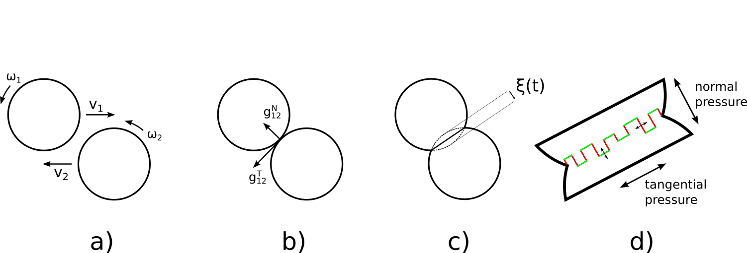
The equations and the figure are written for two particles with radius , , positions , , translational velocities , and rotational velocities , . The relative velocity is defined as where defines the normal direction; we call and the two projections, respectively normal and tangential, to the surface of contact. The instantaneous normal compression is represented by and its derivative is . During the contact, the particles are subjected to a normal force and a tangential one ; both these components have an elastic and a dissipative contribution individuated by the couples of parameters , and , , respectively. In the normal force we can see an elastic term that descends from the Hertzian theory of contact mechanics Popov (2010) characterized by a non-linear dependence on the displacement. We recall that in the framework of the same theory it is also possible to derive the dissipative term Brilliantov et al. (1996). The less intuitive term of the model is surely the elastic-tangential one because it depends upon the memory force that takes into account the past history of the tangential displacement Zhang and Makse (2005). We finally remark that in this model the tangential force is limited by Coulomb friction, characterized by the coefficient (Eq.3).
II Details of the simulation
Now we briefly discuss how we set the interaction parameters and the simulation time step in relation to the properties of the materials in play. The elastic coefficients can be directly derived as
| (4) |
where is the Young modulus and in the Poisson ratio. This holds for contacts between same material but it is possible to generalize to the case of two species Zhang and Makse (2005); Popov (2010); Di Renzo and Di Maio (2004). Direct formulas for and are lacking but it is a common strategy to choose them verifying a posteriori the good agreement with the experimental data T. Pöschel (2005). The simulation time step has been chosen as a fraction of the Rayleigh time namely the time that a superficial acoustic wave takes to cross a single grain. It is related to the characteristics of the material:
| (5) |
where is the grain density and the radius of the littlest grain in the system Rackl and Hanley (2017). This is a good choice to properly resolve the dynamics because is usually much smaller than the typical collision times. We finally report the numeric values of the parameters in the Tab. 1 where superscript is referred to steel and to Plexiglas. It is worth underlining that we choose a Young modulus for the steel that is two order of magnitude smaller than the real one ( Pa). The reason is the need to have a bigger in order to decrease the simulation time. This is a general strategy in DEM simulations when experimental data are available and hence it is possible to verify that the softening of the grains doesn’t affect the underlying phenomenology.
| 210 Mpa | |
|---|---|
| 0.293 | |
| 0.5 | |
| 153 | |
| 355 | |
| 3 | |
| 1 | |
| 33 Mpa | |
| 0.370 |
| 33 Mpa | |
|---|---|
| 0.5 | |
| 611 | |
| 132 | |
| 3 | |
| 1 | |
| 6.75 | |
| 1.35 |
III Effective Packing Fraction Of the system
Here we report a table (Tab. 2) with the average packing fraction of the system corresponding to the most representative values of and .
| 300 | 700 | 1300 | 1600 | 2000 | 2600 | |
|---|---|---|---|---|---|---|
| 19.5 | 13.8 | 24.6 | 39.3 | 45.0 | 51.6 | 56.3 |
| 30.6 | 8.4 | 17.7 | 30.8 | 37.3 | 44.8 | 52.9 |
| 39.8 | 6.4 | 14.5 | 26.7 | 32.8 | 41.1 | 48.8 |
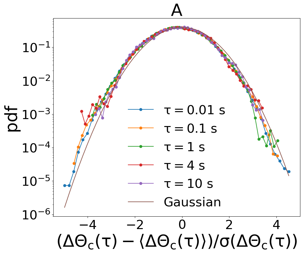
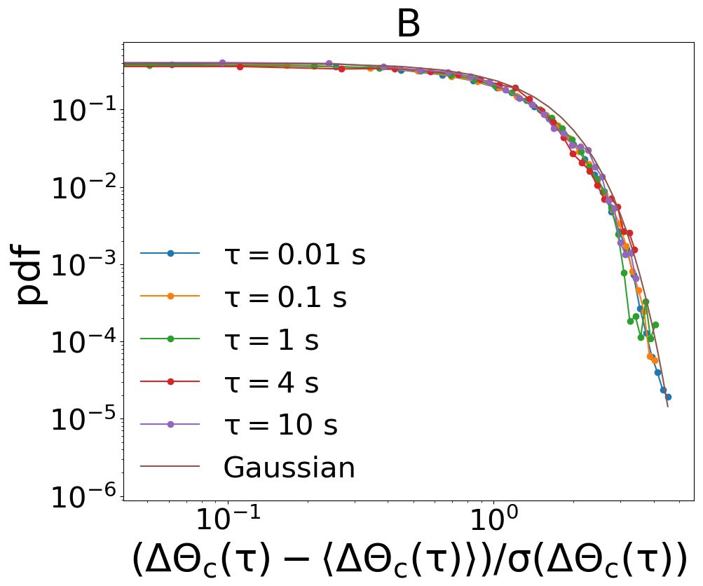
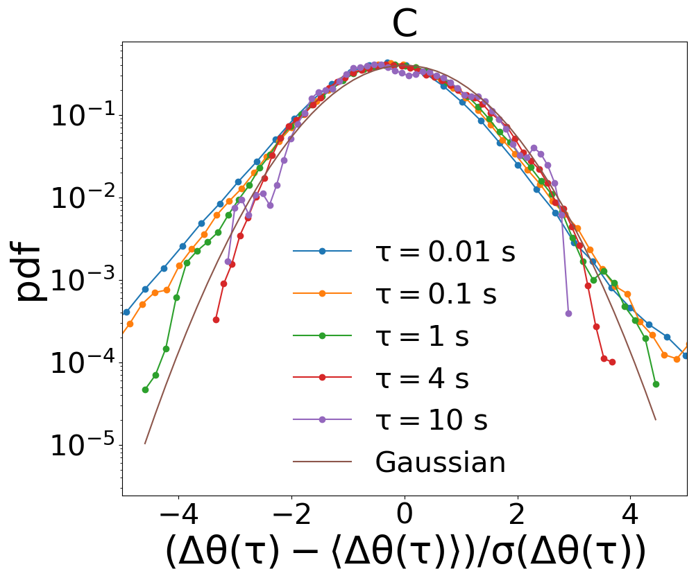
IV Distribution of displacements
The superdiffusion observed for the single particle angular displacement as well as for the collective angular variable , see Figures 4A and 5B of the Letter, is related to long persistence of almost ballistic flights in the system, as documented by the trajectories of the variables (Figs. 1B, 3A and 3C). In order to strengthen our argument, we have measured also the distributions of the displacements: this is useful to rule out an alternative origin of the effect, that is the presence of large (Lévy) tails, such as those observed in Lechenault et al. (2010). Distributions of the collective displacement, shown in Fig. 7A and B, display a Gaussian shape at all delays . Distributions of the single particle displacement - see Fig. 7C and D - on the contrary, have large tails (but certainly with a finite variance) at small times and become Gaussian from times larger than .
V Effects of the main setup’s parameters
In this Section we explore the consequences of changing some parameters of the numerical model, in particular: 1) we reduce the particles’ diameters (at constant density) in order to increase the effective size of the system; 2) we add some polidispersity in the system to rule out possible effects of crystallization; 3) we change the dissipation in the interaction among the grains; 4) we change the mass of the grains.
V.1 System’s size
In Fig. 8 we show the mean squared angular displacement of the collective variable (8A) and of the single particles (8B) when the diameter of the particles is halved and the number is increased by a factor , so that the total average packing fraction remains unaltered. Both collective and single particle msd reveal superdiffusion at large times, with a power (close to ) very similar to the smaller system.
V.2 Polidispersity and crystallization
The long dynamical memory observed in both our real and numerical experiments can be suspected of being related to a strong configurational order in the system. In this subsection we rule out such a hypothesis by means of two key observations. First we check that in our monodisperse simulations the degree of order is below the crystallisation threshold usually considered in the literature. Second, we run new simulations with a polidisperse system, fairly reproducing the same superdiffusion behavior observed in the monodisperse system.
The degree of order in our system is measured by means of a crystallographic order parameter defined in terms of spherical harmonics, which is a usual and reliable observable to distinguish between crystallized and disordered configurations of a many-particle system, see for instance Lechner and Dellago (2008); Russo and Tanaka (2012); Zaccarelli et al. (2009); Pusey et al. (2009). For each particle a complex vector is defined as
| (6) |
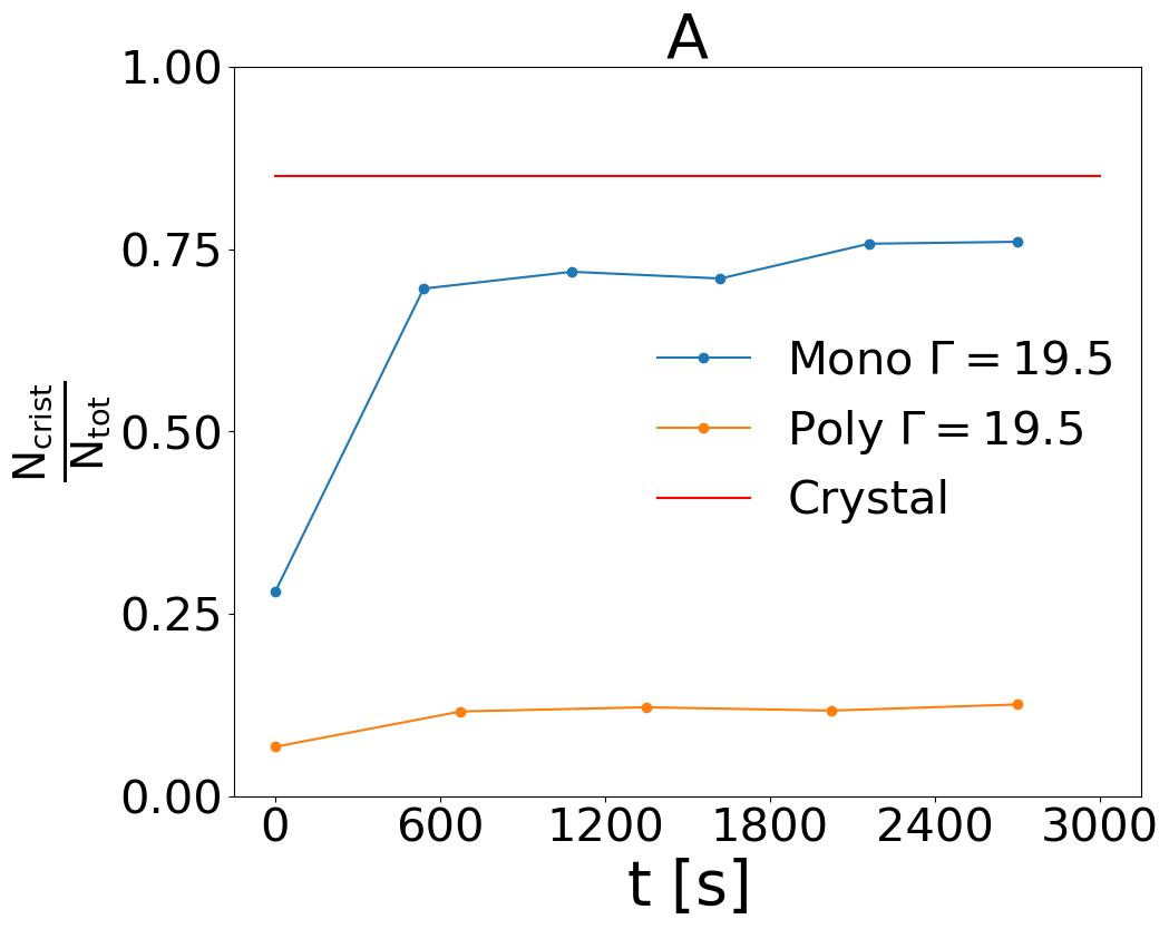
where are the 6th order spherical harmonics with an integer that runs from to , is the number of neighbors of particle (i.e. particles whose distance is smaller than radii) and is the unit vector joining particles and , defining a unique point on the sphere where the spherical harmonic is defined. The scalar product is computed and the couple is considered “connected” if this product exceeds . If the particle is connected to or more neighbors, then it is considered crystallised. The fraction of crystallised particles is shown in Fig. 9A as a function of time, in order to confirm that we are measuring a steady value. In the considered monodisperse case (which is the densest in our series of simulations) we measure a value smaller than or close to , while in the literature a configuration is considered a crystal when such a fraction is larger than .
Then we have run simulations with a significant degree of polidispersity. This is obtained by placing in the container the same number of particles but with random diameters, extracted according to a 9-component discrete Gaussian distribution with average mm and standard deviation equal to of the average. The measure of the crystallographic order, shown in Fig. 9A demonstrates that such a protocol guarantees a significantly smaller percentage of crystallisation, . Nevertheless, the behavior of the system, with superdiffusive mean squared displacement, is fairly recovered, as shown in Fig. 9B.
V.3 Inelasticity and mass of the particles
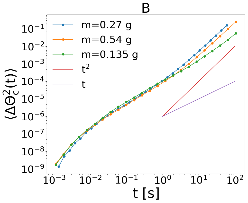
Inelasticity in our model mainly comes from the presence of viscous interaction during contact, see Eqs. (3), embodied in the damping parameters and , for normal and tangential dissipation respectively. Here we change keeping constant the ratio . The effect upon the mean squared angular displacement of reducing the dissipation is shown in Fig. 10A. We do not observe a clear monotonous behavior, but a significant reduction of the superdiffusion phenomenon at smaller dissipation can be excluded. This points at a possible connection with long memory effects observed in elastic dense fluids, for instance the so-called hydrodynamic long time tails in velocity autocorrelations Brenig (1989). It is however interesting to notice that our system lives in three dimensions, where a hard sphere system is expected to display velocity autocorrelations with tails decaying as which are integrable and therefore exclude superdiffusion. In fact superdiffusion in elastic three-dimensional hard sphere systems has not been observed up to our knowledge. Dimensionality, here, is of course not trivial since the angular variables live in an effective single dimension. We also recall that long time tails, of the same kind, are observed also in systems of inelastic hard spheres Fiege et al. (2009).
A more clear and relevant effect on msd, on the contrary, is seen when the mass of the particles is reduced, see Fig. 10B. A system with a mass times smaller appears to have weaker superdiffusion. This seems coherent with our interpretation of the superdiffusive regime as a consequence of large inertia (together with coherence) in the system.