Dynamical disruption timescales and chaotic behavior of hierarchical triple systems
Abstract
We examine the stability of hierarchical triple systems using direct -body simulations without adopting a secular perturbation assumption. We estimate their disruption timescales in addition to the mere stable/unstable criterion, with particular attention to the mutual inclination between the inner and outer orbits. First, we improve the fit to the dynamical stability criterion by Mardling & Aarseth (1999, 2001) widely adopted in the previous literature. Especially, we find that that the stability boundary is very sensitive to the mutual inclination; coplanar retrograde triples and orthogonal triples are much more stable and unstable, respectively, than coplanar prograde triples. Next, we estimate the disruption timescales of triples satisfying the stability condition up to times the inner orbital period. The timescales follow the scaling predicted by Mushkin & Katz (2020), especially at high where their random walk model is most valid. We obtain an improved empirical fit to the disruption timescales, which indicates that the coplanar retrograde triples are significantly more stable than the previous prediction. We furthermore find that the dependence on the mutual inclination can be explained by the energy transfer model based on a parabolic encounter approximation. We also show that the disruption timescales of triples are highly sensitive to the tiny change of the initial parameters, reflecting the genuine chaotic nature of the dynamics of those systems.
1 Introduction
Triple star systems ubiquitously exist in the universe. Observationally, more than 70% of OBA-type stars and 50% of FGK-type stars are known to belong to multiple systems (e.g., Raghavan et al., 2010; Sana et al., 2012), and their multiplicity increases with the mass of stars (Moe & Di Stefano, 2017). The diversity and architecture of triple systems have been studied extensively through recent photometric and spectroscopic observations. For example, 18 triples were recently resolved and their orbital elements determined by combining proper motion and radial velocity (Tokovinin & Latham, 2020; Tokovinin, 2021). Hajdu et al. (2021) discovered 23 triple systems using eclipse time variations with OGLE-IV in eclipsing binaries. More recently, Gaia astrometric survey reported the Data Release 3 (Gaia DR3), and about 100 genuine triple stars were identified from astrometric and spectroscopic solutions (Gaia Collaboration et al., 2022). Gaia DR3 also reported 17 stars with potential compact companions with large mass functions: . These candidates may include binary compact objects, as well as single neutron star and black hole companions. These current observational results are quite interesting, and suggest the importance of studying triple systems both observationally and theoretically.
We are particularly interested in triple systems comprising an inner binary black hole (BBH), which have not yet discovered. While the gravitational wave (GW) observations have revealed that there are abundant populations of massive BBHs in the universe, their formation mechanisms are not well understood; possible scenarios include the evolution outcome of isolated massive binary stars (e.g. Belczynski et al., 2002), dynamical capture of two BHs in dense stellar systems (e.g. Portegies Zwart & McMillan, 2000), and binary assembly from primordial BHs (e.g. Sasaki et al., 2016). Regardless of the details of such scenarios, the progenitors of the observed BBHs are likely to spend a significantly long period as widely separated BBHs before the coalescence. Furthermore, a fraction of those progenitor BBHs may be accompanied by a tertiary that accelerates the merger time through the von Zeipel-Kozai-Lidov (ZKL) oscillations (Blaes et al., 2002; Miller & Hamilton, 2002).
More specifically, Antognini & Thompson (2016) performed million simulations of gravitational scatterings of binary-binary, triple-single, and triple-binary scatterings. They found that the relatively close triples with a few - semi-major axis ratio is efficiently produced from dynamical scattering events. Later, Fragione et al. (2020) performed systematic numerical simulations of dynamical interactions of stars and compact bodies in dense clusters, and found binary-binary encounters efficiently produced stellar and compact triples. In addition, Trani et al. (2021) examines the formation of wide-separate triples via dynamical interactions in young star clusters from simulations performed in Rastello et al. (2020), and found that the ZKL oscillation plays an important role for the coalescence of compact binaries in such triples. For more comprehensive reviews on the formation of merging compact objects, including the triple evolution channel, we refer to Mapelli (2021) and Spera et al. (2022).
In this context, we would like to mention an interesting triple system comprising three compact objects, although not BHs (Ransom et al., 2014). The triple was discovered by the pulsar timing, and consists of an inner binary of a millisecond pulsar (PSR J0337+1715) and white dwarf, and a tertiary white dwarf of . Their inner and outer orbital periods are 1.63 days and 327 days, respectively, and the orbits are nearly coplanar (), and circular (the inner eccentricity and outer eccentricity ). Even though its formation pathway would be very different from triples with inner BBHs, the above system proved the existence of triples consisting of compact objects. Therefore, it is tempting to explore a feasibility to discovering an overlooked population of triples with such an amazing architecture.
These considerations motivated us to propose methodologies to search for BBHs embedded in triple systems through the radial-velocity modulations or the pulsar arrival time delays of tertiary (Hayashi et al., 2020; Hayashi & Suto, 2020, 2021). They are expected to provide a novel method to discover a population of BBHs in optical and radio observations in a complementary fashion to the GW survey. The expected number of such triples with BBHs is very model-dependent and difficult to predict theoretically. Thus a successful discovery of such a triple would have a strong impact in understanding the formation mechanism of BBHs as well.
Once such triples are formed, however, they may not be dynamically stable and become disrupted in a relatively short timescale. Indeed, the orbital stability of triples is one of the long-standing key questions in three-body problems, and there have been many previous studies focusing on this issue. Among others, Mardling & Aarseth (1999, 2001) (hereafter, MA01) proposed a widely used criterion of the dynamical instability of triples. Their criterion was later generalized to include the dependence of inner orbital elements (e.g. Mylläri et al., 2018), or general relativistic corrections (e.g. Wei et al., 2021). More recently, Lalande & Trani (2022) proposed a machine learning method to predict the stability of the hierarchical triples.
In general, those criteria are intended to assess whether a triple is stable or not, but cannot be directly used to predict their disruption timescale. As we will show below, some systems remain bound even for more than times the inner orbit period, depending on their specific orbital configuration. It is important, therefore, to find an expression for the disruption timescale of triple systems.
Mushkin & Katz (2020, hereafter MK20) have presented a physically well-motivated model for that purpose. They particularly focus on a triple system with a highly eccentric outer tertiary, and estimate the disruption timescale by evaluating the energy transfer between the inner and outer orbits based on the Random Walk (RW) assumption. They first consider a full RW model that numerically integrates the secular evolution of triples, and propose an analytic expression for the disruption timescale from a simplified version of the RW model. Their formula reasonably reproduces the numerical results of the disruption time for triples whose outer eccentricity is sufficiently close to unity, and thus the parabolic orbit approximation is justified, but the agreement is significantly degraded otherwise.
The purpose of the present paper is to generalize the result of MK20 and find an empirical fit to the dynamical disruption timescales for hierarchical triple systems over a larger parameter space. Specifically, we proceed according to the following strategies.
-
1.
We perform a series of systematic -body simulations for hierarchical triple systems with various orbital configurations. We do not adopt the conventional orbit-average approximation, but directly simulate three point-mass particles using a fast and accurate -body integrator tsunami (Trani & Spera, 2022).
-
2.
As in MA01 and MK20, we consider Newtonian gravity alone, neglecting general relativity or finite-size effects including spin and tidal interaction of particles.
-
3.
We focus on the three specific values of the mutual inclination : coplanar prograde (), orthogonal (), and coplanar retrograde ().
-
4.
We clarify the chaotic nature of the triple disruption by showing the high sensitivity to the input parameters, and thus attempt to obtain a statistical fit to the numerical results generalizing the RW model proposed by MK20.
-
5.
We directly show that the scaling with respect to the mass and semi-major axis of triples is valid in a statistical manner despite their chaotic behavior of the disruption dynamics.
-
6.
We apply the energy transfer model by Roy & Haddow (2003) to explain why coplanar retrograde triples are the most stable and initially orthogonal triples are the most unstable in general.
The rest of the paper is organized as follows. First, we briefly review a few previous models relevant to the stability and disruption timescales of hierarchical triples in section 2. Next, we describe our numerical methods to integrate the triple systems using the direct -body simulation in section 3. Section 4 focuses on triples comprising an equal-mass inner binary, and discusses how sensitively the chaotic nature of their dynamics changes the estimated timescales. In section 5, we show the stability boundaries and the disruption timescales from our simulation runs, and obtain the improved empirical fits by generalizing the previous models. Section 6 presents examples of evolution of orbital elements, energy, and angular momentum of triple systems, and consider how they depend on the mutual inclination between the inner and outer orbits. Finally, section 7 is devoted to summary and conclusion of the paper. In appendix, we show how our estimates of disruption timescales are affected by the variation of initial phase angles (section A), summarize the ejection pattern (section B), and discuss the possible effect of general relativity that is ignored in the present paper (section C).
2 Previous models for the dynamical stability of triple systems
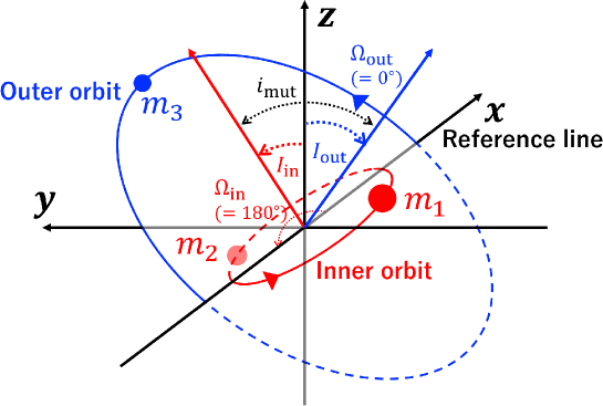
Figure 1 illustrates a schematic configuration of a hierarchical triple system considered in the present paper. The inner binary consists of two massive bodies of and , and a tertiary with mass orbits around the binary. The orbital parameters of inner and outer orbits are specified in terms of the Jacobi coordinates. Each orbit is characterized by the semi-major axis , the eccentricity , and the argument of pericenter . The orientation of orbits in space are specified by the longitude of ascending nodes measured from the reference line, and the mutual inclination between inner and outer orbits.
This section briefly reviews three important previous models that underlie our current approach to estimating the dynamical disruption time of triple systems.
2.1 Dynamical instability criterion by MA01
Mardling (1995a, b); Mardling & Aarseth (1999, 2001) considered evolution of a tidally interacting binary. They defined that a binary evolution is chaotic when the direction and amount of energy flows between the tide and orbit become entirely unpredictable. In reality, the boundary between normal and chaotic behavior is not well defined, since it is extremely sensitive to small differences of orbital parameters and regions of stability and chaos are intertwined in a complicated fashion. Nevertheless, they were able to derive an approximate formula for the boundary.
Remarkably, MA01 recognized that the way of energy and angular momentum exchange between the inner and outer orbits in a hierarchical triple is very similar to that in a tidally interacting binary. On the basis of the analogy, MA01 proposed the following dynamical instability criterion for hierarchical triples:
| (1) |
In the above expression, and are the semi-major axes of the inner and outer orbits, is the eccentricity of the outer orbit, is the mutual inclination between the two orbits, and is the total mass of the inner binary.
The numerical coefficient of 2.8 in inequality (1) is empirically introduced by MA01 from numerical simulations. They define the stability based on whether two orbits, differing by part in in the eccentricity, remain similar after 100 outer orbits. The additional dependence on the mutual inclination, , is heuristically introduced in Aarseth & Mardling (2001) based on the result of stability enhancement due to discussed by Harrington (1972). The extension of this criterion is done by Mylläri et al. (2018) to include the dependence on the mass ratio of the inner binary , the mutual inclination , and the inner eccentricity .
Inequality (1) indicates that the ratio between the pericenter distance of the outer orbit and the semi-major axis of the inner orbit is the key parameter dictating the chaotic behavior of the triples. Triples with are unstable because their outer and inner orbits cross each other. Inequality (1) should be interpreted as a criterion for the onset of chaotic evolution, rather than for disruption, but triples with begin chaotic orbital evolution and are expected to be disrupted eventually. Therefore, while inequality (1) is widely known as a standard criterion for dynamically unstable triples (e.g. Perpinyà-Vallès et al., 2019; Gupta et al., 2020; Tanikawa et al., 2020), it cannot be used to predict the disruption time.
2.2 Random Walk Model by MK20
In order to estimate the disruption time of triples, MK20 apply the random walk (RW) approximation for the energy transfer between the inner and outer orbits. They focus on very eccentric outer orbits (), and use an approximate analytic formula of the energy during the pericenter passages of a parabolic orbit by Roy & Haddow (2003). The transferred energy depends on the inner mean anomaly during the next outer orbital pericenter. Their RW model assumes that the inner mean anomaly changes randomly between adjacent outer pericenter passages without net energy exchange on average. The resulting energy transfer process, therefore, is supposed to be well described by a random walk. Furthermore, they assume that the disruption likely occurs when the accumulated transferred energy variance becomes comparable to the square of the outer orbital energy, and derive the disruption time of triples.
In their full RW model, they perform secular integration numerically up to the quadrupole interaction so as to include the effect of evolving orbital parameters. They also consider a simplified version of the RW model, in which the complicated evolution of orbital elements are neglected. Their simplified RW model yields the following analytic expression for the disruption time :
| (2) |
where is the initial orbital period of the inner binary, and is the total mass of the system.
The factor in equation (2) is heuristically determined from their -body simulations. They found that the RW model estimations can reasonably reproduce the disruption times of numerical simulations within one order-of-magnitude for high- triples; they also perform simulations for , 0.3, 0.5, 0.7, and , and confirm that their models agree well with the simulations down to although the accuracy of equation (2) significantly decreases at lower eccentricities.
2.3 Energy transfer for a parabolic encounter
The energy transfer model adopted by MK20 is based on a binary-single scattering process for a parabolic encounter by Roy & Haddow (2003). Indeed, this model turns out to be important to understand the dependence of the disruption time on the mutual inclination, we briefly summarize the result of Roy & Haddow (2003) in this subsection.
They apply the perturbation theory and compute the energy exchange during an encounter in which the collision parameter is much larger than the semi-major axis of a binary, neglecting rapidly oscillating terms. If the eccentricity of outer orbit is close to unity, the energy transfer during a pericenter passage is well approximated as a binary-single scattering for a parabolic encounter. The energy transfer during one pericenter passage for a triple system is written as (Mushkin & Katz, 2020):
| (3) |
where , , and are the pericenter distance of the outer orbit, the characteristic phase angle, and the relative longitude of the ascending nodes, respectively.
The characteristic phase is defined as
| (4) |
where and are the pericentre argument, and the inner mean anomaly during the passage, respectively. In equation (3),
| (5) |
where
| (6) |
The function in equation (3) is given by
| (7) |
and the dependence on and is explicitly included in the three coefficients:
| (8) | |||||
| (9) | |||||
| (10) |
In the above expressions, are written in terms of the Bessel function of the -th order :
| (11) | |||||
| (12) | |||||
| (13) |
In section 6, we show that the energy transfer is suppressed for retrograde orbits using these expressions, and discuss a possible origin of the dependence of orbital configurations on the disruption timescales.
3 Numerical methods
3.1 Simulation parameters and scaling
As illustrated in Figure 1, there are a number of parameters characterizing triples, and it is not realistic to cover the parameter space systematically. Thus, we adopt a fiducial set of parameters, which is listed in Table 1. The specific choice of is partly motivated by our previous papers (Hayashi et al., 2020; Hayashi & Suto, 2020) that consider a triple comprising an inner BBH and a stellar tertiary. Due to the scaling in the basic equations, however, the result can be easily applied for other cases. More specifically, mass and length, and time scales in purely gravitational problem admit the following scaling relation:
| (14) |
The relation (14) implies that the disruption time computed from our set of simulation runs can be scaled as Indeed, this is why we mostly express our results below in terms of dimensionless variables like .
Therefore, more relevant parameters are the mass ratio of the inner binary , the mass ratio of secondary and tertiary , the outer pericenter distance over inner semi-major axis , the outer eccentricity and the mutual inclination .
In addition to those parameters, the variation of initial phase angles (, , , and ) would introduce statistical variance on . As will be discussed in appendix, we find that the resulting stochastic variance amounts to one or two orders of magnitudes, which is indeed comparable to the level of fluctuations due to the intrinsic chaotic nature of the triple systems that we consider in this paper.
| orbital parameter | symbol | initial value |
|---|---|---|
| inner-binary mass | ||
| inner-binary period | ||
| inner eccentricity | ||
| inner pericenter argument | ||
| outer pericenter argument | ||
| inner longitude of ascending node | ||
| outer longitude of ascending node | ||
| inner mean anomaly | ||
| outer mean anomaly |
Note. — We adopt the above values for input of simulations as our fiducial systems unless otherwise specified. We vary the other parameters including , , , , and as discussed in the main text. Note that is uniquely determined by and , and , and are uniquely determined by , , and .
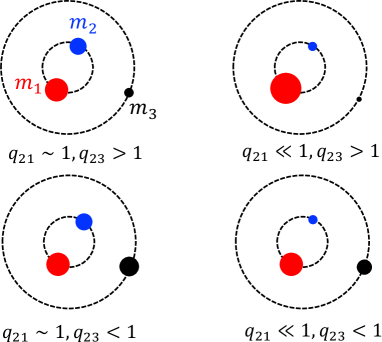
We define the primary as the most massive body in the inner binary (so that ), and thus . While for a hierarchical triple consisting of inner massive binary and a tertiary, we consider cases of as well that are relevant for planetary systems in general. Figure 2 illustrates schematic pictures of triples in different and regimes.
3.2 -body integrator
In order to obtain the disruption time distributions of triples, we perform a series of numerical simulations with the -body integrator TSUNAMI (Trani et al., 2019, Trani et al., in prep.). TSUNAMI is a direct -body integrator specifically designed to accurately simulate few-body systems. The code solves the Newtonian equations of motion derived from a time-transformed, extended Hamiltonian (Mikkola & Tanikawa, 2013a, b). This numerical procedure, also called algorithmic regularization, serves to avoid the well known issue of gravitational integrators when two particles get very close together. When no regularization is employed, the acceleration grows quickly, and the timestep becomes extremely small, sometimes even halting the integration. Specifically, we employ the logarithmic Hamiltonian regularization scheme, which corresponds to setting , , and in the notation of Aarseth, Tout, & Mardling (2008). Furthermore, TSUNAMI is suited to evolve hierarchical systems of particles like the ones examined here, thanks to its chain-coordinate system that reduces round-off errors when calculating distances between close particles far from the center of mass of the system (Mikkola & Aarseth, 1993). Finally, TSUNAMI uses Bulirsch-Stoer extrapolation to improve the accuracy of the integration, ensuring accuracy and adaptability over a wide range of dynamical scales (Stoer & Bulirsch, 2002). As a result, TSUNAMI can perform accurate three-body simulations roughly times faster than other integrators. For more details on the integration scheme, we refer to Trani & Spera (2022).
The definition of the dynamical stability is not unique. Indeed, it may depend on the maximum integration time that we adopt in numerical simulations to some extent. First, we define the disruption time for each triple following Manwadkar et al. (2020, 2021). At each timestep, the integrator evaluates the binding energy for each of the three pairs of bodies, i.e. , and . The pair with the highest (negative) binding energy is considered as the inner binary, and we call the pair of the inner binary and the remaining tertiary as the outer pair. When the binding energy of the outer pair becomes positive and the radial velocity of the tertiary becomes positive (i.e. is moving away from the inner binary), we tentatively regard it as a candidate of a disrupted triple, and assign the epoch as the disruption time . Some of them, however, represent a transient unbound state, and subsequently become gravitationally bound again. Therefore, we continue the run until its binary-single distance exceeds 20 times the binary semi-major axis so as to make sure that it is a truly disrupted triple. In that case, we stop the run, and the triple is classified as disrupted with the previously assigned value of . If a system becomes bound again, on the other hand, we reset the temporarily assigned value of , and keep running the integration of the system.
Finally, we define stable triples as those that do not disrupt and survive until our maximum integration time . We set unless otherwise specified.
Due to the chaotic nature of the system, strict numerical convergence cannot be achieved, and the disruption timescales obtained from our simulation runs should be interpreted in a statistical manner. In §4.2 and appendix A, we attempt a numerical convergence test by running the same set of runs on different machines allowing for a tiny difference of the initial orbital parameter, as well as varying the initial phases of the inner and outer orbits and of the three bodies. In all cases, the disruption timescales agree within one or two orders of magnitudes, indicating that our results are statistically robust within those uncertainties.
4 Qualitative behavior of hierarchical triples comprising an equal-mass inner binary
4.1 Disruption timescales estimated from simulations
This subsection presents our simulation results of the disruption timescales, focusing on triples with an equal-mass inner binary. More general cases will be described in section 5.
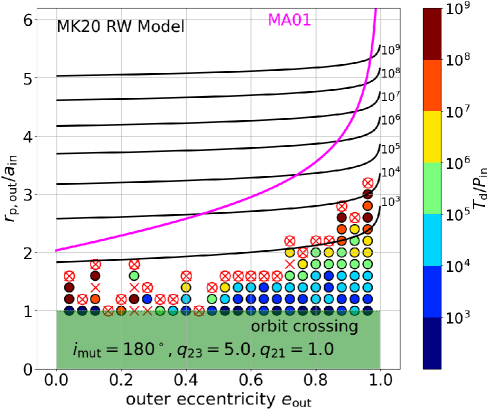
Figure 3 shows the normalized disruption time distribution on - plane for coplanar prograde triples with an equal-mass inner binary (). The secondary to tertiary mass ratio is fixed as , i.e., the tertiary mass is for . We adopt the fiducial values for the other parameters that are listed in Table 1. As discussed in section 4.2, does not exactly scales with because of the scatters inevitably induced by the chaoticity. Nevertheless, is independent of statistically, and we consider the normalized disruption time in what follows.
Triples located above the magenta curves in Figure 3 are expected to be stable according to the MA01 dynamical stability condition. The disruption timescales predicted by the MK20 model are plotted in black contours (for and ). The contours are nearly straight lines on - plane because the exponential term in equation (2) dominates the parameter dependence. The green shaded region in Figure 3 corresponds to the orbit-crossing triples whose outer orbit intersects the inner binary orbit at the pericentre, . Those triples are supposed to be very unstable in general, and are not our main interest in the present paper.
The result of simulated disruption timescales are plotted as filled circles with different colors in Figure 3 according to the side color-scale. We start the simulation with the initial parameters of with the integer running over . For a given value of , we sequentially increase the value of by 0.2. Due to the limitation of the CPU time, we stop each simulation at even if the system is not disrupted, which is approximately equal to Gyrs for our fiducial parameters. For any given , we stop increasing the value of when the previous two realizations at lower do not break before the final integration time. In other words, we scan the - of Figure 3 going from bottom to top, stopping only when two realizations in a row fail to break up before . Thus those triples located above the circle-cross symbols in Figure 3 correspond to . In what follows, we sometimes refer to the boundary as the simulated stability boundary just for convenience.
Figure 3 shows that the MA01 dynamical stability condition, inequality (1), roughly explains the stability boundary of the simulated coplanar prograde triples with an equal-mass inner binary; all triples with are stable at least until .
The predicted disruption timescales based on the MK20 RW model agree well with the simulation result only for triples with . This is indeed expected because their model assumes that the energy transfer between the inner and outer orbits is approximated by a random walk for a highly eccentric outer orbit. MK20 also confirmed that their RW model reproduces their simulations reasonably well down to , which is consistent with our present result. The right panel in Figure 3, furthermore, implies that the lower limit of where the RW model approximation is valid becomes larger as increases.
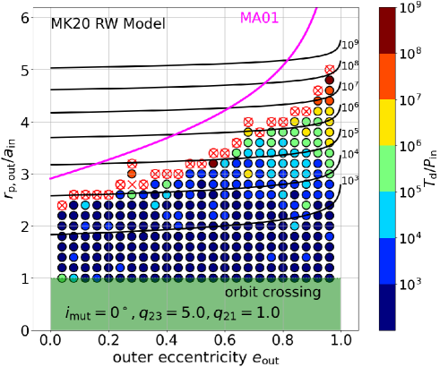
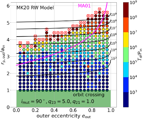
In reality, however, the above rough agreement between the theoretical predictions and simulations does not hold for orthogonal () and coplanar retrograde () cases; see Figures 4 and 5.
Orthogonal triples are less stable than the MA01 criterion, which may be due to their drastic orbital evolution. In particular, the effect of the ZKL oscillation is not properly taken into account in the MA01 model. In contrast, the MK20 RW model seems to agree better than the prograde simulations for even lower values of . Finally, Figure 5 clearly indicates that coplanar retrograde triples are significantly more stable than MA01 and MK20 predict. We will discuss this point later based on the energy transfer model by Roy & Haddow (2003).
4.2 Chaotic nature of triple dynamics and the scaling relation
The results in Figures 3 to 5 are computed initially for a set of fixed phase parameters including mean anomalies (, ) and arguments of pericenter (, ). While all those initial parameters are mixed up in the course of the dynamical evolution, their different values at the initial epoch are likely to affect the disruption timescales to some extent, and to introduce statistical scatters in the estimated timescales. This is quite expected, and we show in appendix A that those phase angles change the disruption timescales by one or two orders of magnitudes.
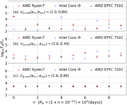
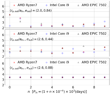
Instead, this subsection addresses the question how the disruption timescale is sensitive to the (tiny) difference of the initial orbital parameters, given the chaotic nature of the gravitational many-body systems in general (e.g., Suto, 1991). For this purpose, Figure 6 examines quantitatively to what extent the disruption timescale is affected by the tiny difference of the initial period of the inner binary.
We select three sets of runs from our fiducial model simulation, and change the initial value of (and therefore that of ) alone while keeping the other parameters intact. In practice, we change the initial input value of days only by its 15-th digit (left panels) and 4-th digit (right panels), which are the horizontal axes of Figure 6, i.e., and . We also repeat the identical run on three different machines; AMD Ryzen7 Core in CfCA calculation cluster at NAOJ, Intel Core i9 on 16-inch Macbook Pro 2019, and AMD EPYC 7502 in our local computer cluster. In this subsection, we stop the runs at to save computational time.
Let us look at the left panels of Figure 6 first. The bottom panel corresponds to a case that the disruption time is insensitive to such a small change. The cases plotted in the top and middle panels, in contrast, indicate that varies significantly among different machines; tiny differences in lead to even by a few orders of magnitudes. This amazing sensitivity to the initial condition originate from the intrinsically chaotic nature of the gravitational dynamics of triples. The variability among different machines is instead due to the limits of floating-point arithmetic and the differences in optimizing compilers that result in slightly different machine code being generated. Together with the extreme sensitivity to initial conditions, these factors cause the introduction of “numerical chaos”, when small but different accumulations of integration errors result in a completely different evolution of the same system.
We repeated those runs except that we modify only the 4-th digit of the initial . The result is shown in the right panels of Figure 6, which are very similar to the left panels. For a triple whose is insensitive to the 15-th digit of the input (the bottom panels), the value is identical in the three different machines even if the 4-th digit is modified, implying that the disruption of the triple seems to proceed in a regular, instead of chaotic, fashion. We could speculate that the Lyapunov time of such system is so long that even a relatively large change in the initial conditions does not result in a different evolution. In contrast, the range of variance of is statistically the same between the left and right panels for the top and middle examples, suggesting that their chaotic nature is fairly independent of the fluctuation amplitude of the input . Such a chaotic degree of the unstable triples is extremely sensitive to the set of orbital parameters in a complicated fashion, and is difficult to predict. Nevertheless, Figure 6 indicates that the disruption timescales from our current simulations should be understood to vary by one or two orders of magnitudes, in practice.
The disruption timescale should admit the scaling relation, equation (14), with respect to and , as long as non-Newtonian effects are neglected. For instance, the RW model prediction, equation (2), respects the scaling. In reality, however, the numerical results do not necessarily satisfy the scaling due to the intrinsic chaoticity described in the above.
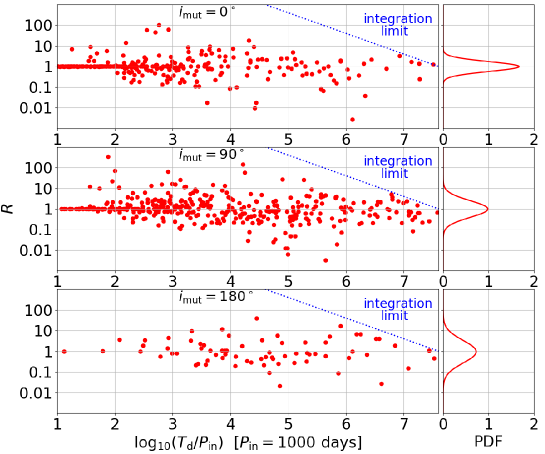
In order to see this, we run simulations for a subset of fiducial triple systems corresponding to Figures 3 to 5 except that we change the value of from days to days (note that is derived from the other fixed parameters). We define the ratio of the normalized disruption timescales for individual triples of and days:
| (15) |
Figure 7 plots against for prograde (top), orthogonal (middle), and retrograde (bottom) triples with and . In order to save the CPU time, we adopt in those examples.
The ratios derived from simulations are not exactly equal to unity due to the chaotic behavior of the triple dynamics, but they distribute around unity in a statistical sense. For instance, we find that their distribution is well approximated by log-normal functions as indicated in the right panels.
In summary, we find that the numerically estimated disruption timescales are inevitably affected by the chaotic behavior of triple dynamics. The timescales may vary one or two orders of magnitudes due to the differences of the initial phase angles and also to the tiny changes in the other orbital parameters. Nevertheless, we conclude that the disruption timescales are statistically robust, and can be predicted from the orbital parameters within one or two order-of-magnitude uncertainty.
5 Comparison with simulated disruption times and previously proposed models: prograde, orthogonal, and retrograde orbits
Having in mind the scatter of the simulated disruption timescales that we discussed in subsection 4.2, we present a detailed comparison of the simulation results against the previous theoretical models (MA01 and MK20). In particular, we examine the dependence on the mutual inclination between the inner and outer orbits. For definiteness, we focus on the three cases including coplanar prograde (), orthogonal (), and coplanar retrograde () triple systems. For each case, we consider and , and , , and . We perform simulations for those 18 orbital configurations in total, by varying and as described in section 4.1.
5.1 The stability boundary in the - plane
Figures 3 to 5 suggest that there is a fairly sharp boundary of the triple stability on plane. The boundary seems to be roughly approximated by shifting inequality (1) along the vertical direction. Thus, we empirically introduce the coefficient to the MA01 model, and fit the simulated stability boundary as
| (16) |
The results are shown in Figures 8 to 10, together with the value of .
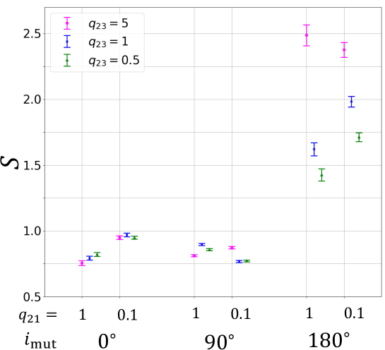
Although equation (16) is a simple extrapolation of the MA01 model, its dependence reproduces the numerical results reasonably well by fitting the value of , especially given the expected scatters discussed in subsection 4.2. The boundaries between stable and unstable regions appear to be very sharp especially for and becomes gentle for , at least for and (Figures 8 and 10). Unlike inequality (1), however, the stability boundary does not monotonically depend on the mutual inclination , and the orthogonal triples are more unstable than the other two coplanar configurations; see Figure 9. In all cases, the disruption timescales for those triples with are mainly determined by the value of , in agreement with the MK20 model.
Figure 11 plots the best-fit values of , which clearly shows the parameter dependence of the stability boundaries in Figures 8 to 10. The fit is not so good in some cases, especially for orthogonal triples. Nevertheless, we perform the least-square fitting for them, and plot the best-fit values of in Figure 11, so as to indicate the approximate behavior of the stability boundary in a qualitative sense. The poor fit for orthogonal triples may imply the importance of their complicated orbital evolution due to the ZKL oscillation; see section 6. Relative to the MA01 criterion, orthogonal triples are more unstable and coplanar retrograde triples are more stable. The dependence on is not well represented by the combination of alone. These differences may likely come from the fact that their model is based on the simulations up to , which is much shorter than our . Of course, it simply reflects the progress of computational resources over the last two decades, and we would like to emphasize the amazing insight and quality of the pioneering work by MA01. We plan to explore the dependence of the dynamical stability boundary on , and in detail and report the result elsewhere.
5.2 Empirical fit to the disruption timescales
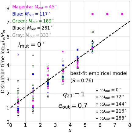
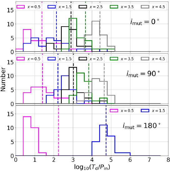
We find that there is a relatively clear boundary between dynamically stable and unstable regions on plane. The boundary is reasonably well approximated by equation (16), which is a simple generalization of the MA01 model. In the unstable regions, the disruption timescales seem to be roughly consistent with the MK20 model. Thus, following equation (2), we introduce a parameter :
| (17) |
Then, equation (2) is rewritten in terms of as follows, which clearly implies that the value of basically determines the disruption time:
| (19) | |||||
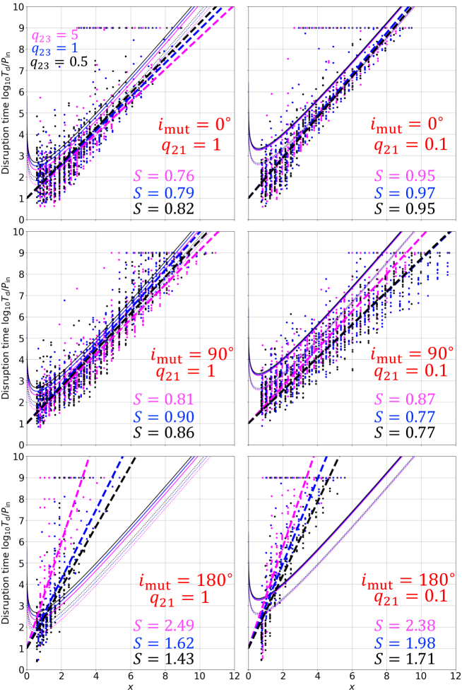
Figure 12 compares the distribution from our simulation against the MK20 model; top, middle, and bottom panels show the prograde (), orthogonal (), and retrograde cases (), while left and right panels are for equal-mass () and unequal-mass inner binaries. The results with different are plotted in different colors: (magenta), (blue), and (black). Thin solid and dotted lines indicate the MK20 model predictions, equation (19), for and , respectively, so as to bracket the dependence on . Filled circles in different colors correspond to our simulation data in Figures 8 to 10. The sequence of data located at corresponds to triples that are dynamically stable up to our integration time , and thus are not considered in the discussion below.
Let us examine more quantitatively Figure 12. Coplanar prograde triples (top panels) do not exhibit noticeable dependence on in the range - , which is consistent with the very weak dependence on that the MK20 model predicts. Furthermore, unequal-mass inner binaries () tend to be slightly more stable than equal-mass ones, which is in a qualitative agreement as well with the MK model.
Orthogonal triples (middle panels) exhibit no strong dependence on either, given the large scatters of simulated data, while unequal-mass inner binaries seem to be more stable for less massive tertiaries (with ) in contrast to the MK20 model. This may indicate the importance of other processes than the RW energy transfer, such as the ZKL oscillation up to octupole interaction. In section 6, we show one typical orbital evolution under the ZKL oscillation.
Coplanar retrograde triples (bottom panels), on the other hand, are significantly more stable than the above two cases, and behave very differently relative to the MK20 model, as already indicated in Figures 8 to 10. The fact that simply reversing the motion of the outer body changes significantly the disruption time distribution is not so intuitive, and we will discuss further in the next section.
Since we have not yet identified physical processes that explain the orbital configuration dependence on the disruption time, we introduce a simple empirical model, and determine the best-fit parameters to summarizes our current results. For that purpose, we consider the following parameterization:
| (20) |
where the dominant term in the MK20 RW model corresponds to .
We first attempted to fit the results of Figure 12 by varying and , and found that most of the results are fitted with close to unity. Given the scatters of the disruption timescales due to the initial phase angles and chaotic behavior of the triples, therefore, we decided to adopt and fit with alone. Thick-dashed lines in Figure 12 represent the best-fit models corresponding to equation (20) with . Figure 13 shows the best-fit value and the associated 1-confidence for . While equation (20) is a very rough approximation, it depicts our simulation results at least qualitatively, and is helpful to understand their basic behavior in a simple way.
6 Orbital evolution of hierarchical triples with different mutual inclinations
We have shown that the disruption timescales are very sensitive to the mutual inclination between the inner and outer orbits. In order to understand their disruption processes, we first show how various orbital elements in our numerical simulations evolve differently according to the mutual inclination. Then, we explain why the orthogonal triples are more unstable, and the retrograde triples are more stable than the coplanar triples, applying the energy transfer model between the two orbits for a parabolic encounter approximation by Roy & Haddow (2003).
6.1 Evolution of orbital elements, energies, and angular momenta
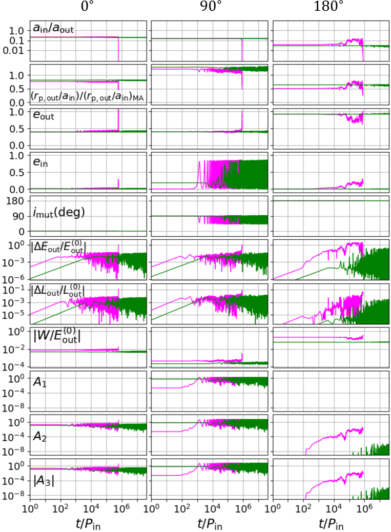
Evolution of orbital elements, energies and angular momenta for hierarchical triples with and is plotted in Figure 14. Left, middle and right panels are for the coplanar prograde, orthogonal, and coplanar retrograde triples. In each panel, magenta and green curves represent the evolution of systems that disrupt around and remain stable at , respectively.
From top to bottom panels, we plot the semi-major axis ratio of the inner and outer orbits , the ratio of and the MA01 threshold , the outer eccentricity , the inner eccentricity , the mutual inclination , the fractional variation of the total energy and angular momentum of the outer orbit and , , and finally ( equations 8–9) and (equation 10).
Both coplanar triples remain coplanar for the entire evolution, and their inner eccentricities are relatively small. In contrast, the initially orthogonal triple changes the mutual inclination between and due to the ZKL effect, which is accompanied by the large periodic oscillation of . As we will show in the next subsection, this is why the initially orthogonal triples are more unstable than the coplanar cases.
After a certain period of the energy transfer between the inner and outer orbits, drops and is enhanced suddenly for unstable cases, leading to an ejection of the tertiary.
6.2 Dependence of the energy transfer on the mutual inclination
The fact that the disruption timescales are sensitive to the mutual inclination angle between the inner and outer orbits may be understood from the model by Roy & Haddow (2003), which is briefly summarized in section 2.3. Specifically, equations (3) and (7) indicate that the energy exchange between the inner orbit and a parabolic perturber is approximately estimated as
| (21) |
where is given by equation (5).
Let us assume that the energy transfer between the inner and outer orbits in our hierarchical triples is approximated by such an encounter, which happens periodically at a pericenter of the eccentric outer orbit.
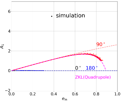
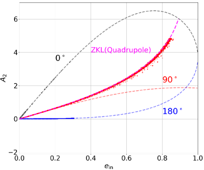
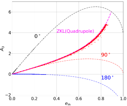
The coefficients to are explicitly given by equations (8) to (13), and plotted in Figure 15 against for (solid), (dotted), and (dashed). Expanding those equations with respect to , one obtains their leading-order expressions as
| (22) |
Equation (22) and three curves in Figure 15 seem to suggest that orthogonal triples are more stable than coplanar prograde triples if compared at the same value of . In reality, however, our simulation runs indicate that the orthogonal triples are the most unstable. This is due to the fact that the inner eccentricity significantly varies for orthogonal triples due to the ZKL oscillation, thus we have to take account of the evolution of as well. From the conservation of the total angular momentum in the ZKL effect, one can derive the relation (e.g. Naoz, 2016):
| (23) |
for triples initially with and . In the quadrupole approximation (or in the case of equal-mass inner binaries that do not have the octupole term), and are constant, and equation (23) directly predicts as a function of . Dots in Figure 15 are sampled from the orbital evolution of the models shown in Figure 14, and are in good agreement with the prediction based on equation (23); orthogonal triples exhibit a wide range of , while in the other two coplanar cases, is constant and stays smaller than 0.3 at most. Thus, the behavior of along the real orbital evolution of the three models nicely explains why the orthogonal triples are the most unstable.
7 Summary and conclusion
This paper has examined the stability of hierarchical triple systems using direct -body simulations without adopting a secular perturbation assumption. We have estimated their disruption timescales in addition to the mere stable/unstable criterion, with particular attention to the mutual inclination between the inner and outer orbits. The simulation results have been intensively compared with the previous models including the dynamical stability criterion by Mardling & Aarseth (1999, 2001), and the random walk disruption model by Mushkin & Katz (2020) among others. Our main findings are summarized as follows.
-
1.
We confirmed that the dynamical stability criterion pioneered by Mardling & Aarseth (1999, 2001) captures the basic trend of our simulation results. Since we performed our simulation runs significantly longer than their previous ones, however, we are able to improve the accuracy of the overall amplitude of the stability boundary. Especially, we found that the stability boundary is very sensitive to the mutual inclination in a more complicated fashion than the empirical fit by Mardling & Aarseth (2001); coplanar retrograde triples and orthogonal triples are much more stable and unstable, respectively than coplanar prograde triples (section 5.1).
-
2.
We computed the disruption timescales of triples satisfying the stability condition up to . The timescales follow the scaling predicted by Mushkin & Katz (2020), especially with high where the random walk assumption is supposed to be valid. We obtained an improved empirical fit to the disruption timescales, which also indicated the coplanar retrograde triples are significantly more stable than the previous prediction (section 5.2). We successfully explained this tendency and also why the initially orthogonal triples are the most unstable, applying the energy transfer model for a parabolic encounter developed by Roy & Haddow (2003, section 6.2).
-
3.
We explicitly demonstrated that the disruption timescales, and even the disruption occurrence, are dependent on the initial values of phase angles including the mean anomalies and apsidal orientations of the inner and outer orbits, and vary within a few orders of magnitudes (section 4.2 and appendix A). Additionally, variations of these angles can even turn a stable system into an unstable one and vice versa. This is somewhat expected, but can be evaluated with the long-term direct -body runs without resorting to the secular perturbation approximation, thanks to the recently developed -body integrator TSUNAMI (Trani et al., 2019; Trani & Spera, 2022, Trani et al., in prep.). Perhaps more surprising is the high sensitivity to the tiny change of the initial parameters such as ; even the level of the numerical truncation error seems to change the disruption timescales by a couple of orders of magnitude. This reflects the intrinsic chaotic nature of the dynamics of the hierarchical triple systems, implying that the disruption timescales estimated by the present paper needs to be understood in a statistical sense.
Hierarchical triples have been proposed as one possible channel to accelerate the merger of compact objects via the ZKL oscillation (e.g. Liu & Lai, 2018; Trani et al., 2021). Our result shows that the orthogonal triples, for which the ZKL oscillation are highly efficient, are generally more unstable than previously thought (Mardling & Aarseth, 2001). Therefore, the validity of this channel needs to be considered with the constraint on the disruption timescales as well.
Retrograde triples may be also important as feasible targets of survey for triple systems that include compact inner binaries, as discussed in our previous studies (e.g. Hayashi et al., 2020). Such triples may form via few-body encounters in star clusters, and the predicted mutual inclinations have uniform distribution in (e.g. Fragione et al., 2020; Trani et al., 2021). Thus, once retrograde triples form via this process, they are expected to stay in a stable configuration for a longer time than the coplanar prograde triples.
In this paper, we only take account Newtonian gravity and neglect GR corrections. As discussed in the appendix C, GR corrections may play an important role only for specific orbital configurations. However, GR correction, especially GW emissions, are very important to study different processes leading the disruption of triples, such as inner binary mergers. We plan to consider this process separately, which will be reported elsewhere.
Finally, we would like to note that hierarchical triples include a variety of systems. For example, stars with a binary planet and triple black holes are also interesting systems, although (and exactly because) they have not been discovered yet. Extrasolar binary planets may be detected eventually via transit observations (e.g. Lewis et al., 2015). In order to model the orbital stability of such systems, and study the feasibility of detection, it is important to consider the disruption timescales of such systems, and extend stability models for triple systems to a variety of orbital configuration, including mutual inclination, mass ratios, and other orbital parameters.
After completing the draft of the present paper, we noticed a very recent preprint by Vynatheya et al. (2022). They improved the stability criterion by Mardling & Aarseth (2001), applied machine learning to distinguish between the stable and unstable hierarchical triples, analogously to Lalande & Trani (2022), but did not examine their disruption timescales as we extensively discussed in the present work. The quantitative comparison with their result will be presented elsewhere.
Acknowledgments
T.H. and Y.S. are grateful to Hideki Asada for his hospitality during their visit at Hirosaki University, where part of the present work was performed. Y.S. also thanks Taksu Cheon for his hospitality at Kochi University of Technology. The numerical simulations were carried out on the local computer cluster awamori, and the general calculation server from Center for Computational Astrophysics (CfCA), National Astronomical Observatory of Japan (NAOJ). This work is supported partly by the Japan Society for the Promotion of Science (JSPS) Core-to-Core Program “International Network of Planetary Sciences”, and also by JSPS KAKENHI grant Nos. JP18H01247 and JP19H01947 (Y.S.), JP21J11378 (T.H.), and JP21K13914 (A.A.T). T.H. acknowledges the support from JSPS fellowship.
Appendix A Disruption timescales for triples: dependence on initial phase angles
We computed the disruption timescales of triples by fixing the initial phase angles, but we expect that varying them would add further variations and scatters in the resulting distribution. In order to examine the effect of initial phases, we repeated the runs for coplanar prograde triples with , , and but varying the mean anomaly and pericenter argument of the tertiary, and . The result is shown in Figure 16. For each value of –, we compute realizations by varying the initial outer mean anomaly and the pericentre argument : deg, where and runs over –. For simplicity, we fix the inner angles and . In order to save the CPU time, we adopt here.
As expected, the initial phases change the disruption timescales for unstable triples mostly within one or two order-of-magnitude. We also performed similar runs for orthogonal and coplanar retrograde triples, and plotted the histograms of in Figure 17; initially coplanar prograde (top), orthogonal (middle), and coplanar retrograde (bottom). The figure implies that our result in the main text is confirmed statistically, within one or two order-of-magnitude scatters similar to those coming from the chaotic behavior of those triples.
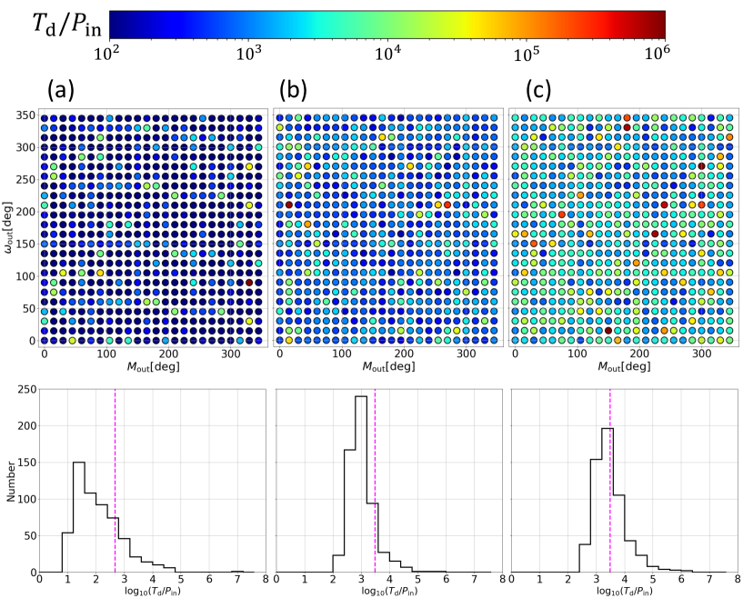
Furthermore, we examine how the initial phases affect the the disruption timescales. For that purpose, we consider the three specific examples corresponding to panels (a), (b), and (c) in Figure 6 with days. Then, we vary their initial phases systematically between and in grids of . The resulting disruption timescales are plotted in Figure 18 on - plane (top), together with the corresponding histograms (bottom). Those plots show that the disruption timescales vary with the initial phases, within one or two order-of magnitudes. The sensitivity to the initial phase dependence does not seem to be directly correlated to the chaotic behavior that is clearly shown in Figure 6; the panel (c) exhibits the similar scatters of the disruption timescale as the other two cases, while it does not show any chaotic behavior against the tiny change in the initial .
Appendix B Ejection pattern of three bodies
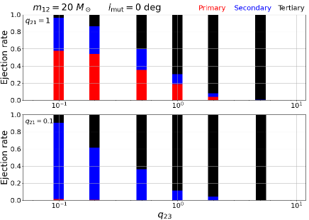
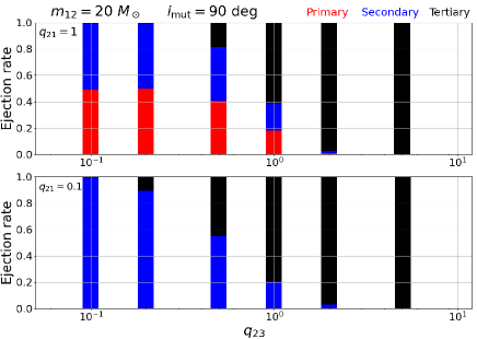
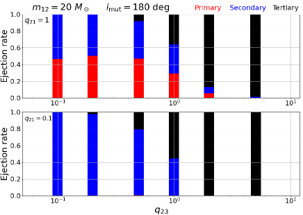
Our result indicates that the disruption timescales and stability boundary are sensitive to the mutual inclinations, but very weakly on and . In order to examine the dependence on and from a different point of view, we show the fraction rate of bodies that are ejected from disrupted triples in Figure 19.
The primary ejection, secondary ejection, and tertiary ejection, are color-coded in red, blue, and black, respectively. In order to save the computational cost, we here adopt . Top, middle, and bottom panels show the results for prograde, orthogonal, and retrograde triples, respectively. Each panel contains the result for (upper) and (lower). We note that there is no physical reason to distinguish between the primary and secondary for , and the small difference in their ejection rate should simply come from statistical reasons.
As expected, the tertiary is preferentially ejected for as the value of increases. The inner less massive body starts to dominate the ejection rate when . The dependence on is stronger for retrograde triples, which is is indeed consistent with Figures 12 and 13.
Appendix C The timescales of GR precessions and GW emissions
We discuss briefly the possible effects of general relativity (GR) that we neglect in the present analysis by considering the GR precession and gravitational-wave emission timescales.
It is known that both the quadrupole and octupole ZKL oscillation is strongly suppressed when the GR precession rate becomes comparable to the ZKL precession rate . The ratio between the two precessions is explicitly given as (e.g. Liu et al., 2015):
| (C1) | |||||
where is the speed of light, and is the Schwarzschild radius of inner binary as if it would be a single body. The estimate above was calculated using the initial conditions of our fiducial triple (see table 1). Thus, it is not likely that GR precession affects the evolution too much except for very massive or close inner binary. Since GR precession suppresses the ZKL oscillation, preventing the oscillations in eccentricity that cause orthogonal triples to be more unstable (see figure 15), GR precession may tend to stabilize the triples in general.
In addition, the long-term GW emission shrinks the orbit of the inner binary. Thus, it reduces the gravitational interaction between the inner and outer orbits, resulting in the stabilization of triples. The typical GW emission timescale may be characterized by the following merger timescale (Peters, 1964) for a circular inner binary:
| (C2) | |||||
where is the initial inner semi-major axis, and we assume our fiducial triple of au. Thus, it is not likely that GW emission affects the evolution for systems without the ZKL oscillation except for a very massive and close inner binary for circular case. On the other hand, the eccentricity might be enhanced by the ZKL oscillations in highly inclined triples. The increase in eccentricity can strongly decrease the coalescence timescale of the inner binary. Given the maximum eccentricity reached during a ZKL cycle, the merger timescale can be expressed as (e.g. Liu & Lai, 2018):
| (C3) |
If we set , the merger timescale decreases by eleven order-of-magnitudes. Thus, the combination effect of the instability from the ZKL oscillation and stabilization from GW emission would be very important to understand the stability of triples for and .
Alternatively, the dynamical instability itself may trigger the enhancement of the eccentricity of the inner binary, or even lead to a temporary state in which no stable binary exist, but all three bodies interact gravitationally with each other. During such states, defined in the literature as democratic resonances (Hut & Bahcall, 1983), two BHs may obtain very close separation so that a merger ensues. This model of gravitational wave coalescence has been extensively studied in the context of three-body encounters in dense environments (e.g. Di Carlo et al., 2020), but also in the context of destabilized field triples (e.g. Toonen et al., 2021).
References
- Aarseth & Mardling (2001) Aarseth, S. J., & Mardling, R. A. 2001, Astronomical Society of the Pacific Conference Series, Vol. 229, The Formation and Evolution of Multiple Star Systems, ed. P. Podsiadlowski, S. Rappaport, A. R. King, F. D’Antona, & L. Burderi (Astronomical Society of the Pacific), 77
- Aarseth, Tout, & Mardling (2008) Aarseth, Sverre J., Tout, Christopher A. & Mardling, Rosemary A. 2008, in The Cambridge N-Body Lectures
- Antognini & Thompson (2016) Antognini, J. M. O., & Thompson, T. A. 2016, MNRAS, 456, 4219, doi: 10.1093/mnras/stv2938
- Belczynski et al. (2002) Belczynski, K., Kalogera, V., & Bulik, T. 2002, ApJ, 572, 407, doi: 10.1086/340304
- Blaes et al. (2002) Blaes, O., Lee, M. H., & Socrates, A. 2002, ApJ, 578, 775, doi: 10.1086/342655
- Di Carlo et al. (2020) Di Carlo, U. N., Mapelli, M., Giacobbo, N., et al. 2020, arXiv e-prints, arXiv:2004.09525. https://arxiv.org/abs/2004.09525
- Fragione et al. (2020) Fragione, G., Martinez, M. A. S., Kremer, K., et al. 2020, arXiv e-prints, arXiv:2007.11605. https://arxiv.org/abs/2007.11605
- Gaia Collaboration et al. (2022) Gaia Collaboration, Arenou, F., Babusiaux, C., et al. 2022, arXiv e-prints, arXiv:2206.05595. https://arxiv.org/abs/2206.05595
- Gupta et al. (2020) Gupta, P., Suzuki, H., Okawa, H., & Maeda, K.-i. 2020, Phys. Rev. D, 101, 104053, doi: 10.1103/PhysRevD.101.104053
- Hajdu et al. (2021) Hajdu, T., Borkovits, T., Forgács-Dajka, E., Sztakovics, J., & Bódi, A. 2021, MNRAS, doi: 10.1093/mnras/stab2931
- Harrington (1972) Harrington, R. S. 1972, Celestial Mechanics, 6, 322, doi: 10.1007/BF01231475
- Hayashi & Suto (2020) Hayashi, T., & Suto, Y. 2020, ApJ, 897, 29, doi: 10.3847/1538-4357/ab97ad
- Hayashi & Suto (2021) —. 2021, ApJ, 907, 48, doi: 10.3847/1538-4357/abcec6
- Hayashi et al. (2020) Hayashi, T., Wang, S., & Suto, Y. 2020, The Astrophysical Journal, 890, 112, doi: 10.3847/1538-4357/ab6de6
- Hut & Bahcall (1983) Hut, P., & Bahcall, J. N. 1983, ApJ, 268, 319, doi: 10.1086/160956
- Lalande & Trani (2022) Lalande, F., & Trani, A. A. 2022, arXiv e-prints, arXiv:2206.12402. https://arxiv.org/abs/2206.12402
- Lewis et al. (2015) Lewis, K. M., Ochiai, H., Nagasawa, M., & Ida, S. 2015, ApJ, 805, 27, doi: 10.1088/0004-637X/805/1/27
- Liu & Lai (2018) Liu, B., & Lai, D. 2018, ApJ, 863, 68, doi: 10.3847/1538-4357/aad09f
- Liu et al. (2015) Liu, B., Muñoz, D. J., & Lai, D. 2015, MNRAS, 447, 747, doi: 10.1093/mnras/stu2396
- Manwadkar et al. (2021) Manwadkar, V., Kol, B., Trani, A. A., & Leigh, N. W. C. 2021, MNRAS, 506, 692, doi: 10.1093/mnras/stab1689
- Manwadkar et al. (2020) Manwadkar, V., Trani, A. A., & Leigh, N. W. C. 2020, MNRAS, 497, 3694, doi: 10.1093/mnras/staa1722
- Mapelli (2021) Mapelli, M. 2021, in Handbook of Gravitational Wave Astronomy (Springer Singapore), 4, doi: 10.1007/978-981-15-4702-7_16-1
- Mardling & Aarseth (1999) Mardling, R., & Aarseth, S. 1999, in NATO Advanced Science Institutes (ASI) Series C, Vol. 522, NATO Advanced Science Institutes (ASI) Series C, ed. B. A. Steves & A. E. Roy (Springer), 385
- Mardling (1995a) Mardling, R. A. 1995a, ApJ, 450, 722, doi: 10.1086/176178
- Mardling (1995b) —. 1995b, ApJ, 450, 732, doi: 10.1086/176179
- Mardling & Aarseth (2001) Mardling, R. A., & Aarseth, S. J. 2001, MNRAS, 321, 398, doi: 10.1046/j.1365-8711.2001.03974.x
- Mikkola & Aarseth (1993) Mikkola, S., & Aarseth, S. J. 1993, Celestial Mechanics and Dynamical Astronomy, 57, 439, doi: 10.1007/BF00695714
- Mikkola & Tanikawa (2013a) Mikkola, S., & Tanikawa, K. 2013a, MNRAS, 430, 2822, doi: 10.1093/mnras/stt085
- Mikkola & Tanikawa (2013b) —. 2013b, New A, 20, 38, doi: 10.1016/j.newast.2012.09.004
- Miller & Hamilton (2002) Miller, M. C., & Hamilton, D. P. 2002, ApJ, 576, 894, doi: 10.1086/341788
- Moe & Di Stefano (2017) Moe, M., & Di Stefano, R. 2017, ApJS, 230, 15, doi: 10.3847/1538-4365/aa6fb6
- Mushkin & Katz (2020) Mushkin, J., & Katz, B. 2020, MNRAS, 498, 665, doi: 10.1093/mnras/staa2492
- Mylläri et al. (2018) Mylläri, A., Valtonen, M., Pasechnik, A., & Mikkola, S. 2018, MNRAS, 476, 830, doi: 10.1093/mnras/sty237
- Naoz (2016) Naoz, S. 2016, ARA&A, 54, 441, doi: 10.1146/annurev-astro-081915-023315
- Perpinyà-Vallès et al. (2019) Perpinyà-Vallès, M., Rebassa-Mansergas, A., Gänsicke, B. T., et al. 2019, MNRAS, 483, 901, doi: 10.1093/mnras/sty3149
- Peters (1964) Peters, P. C. 1964, Physical Review, 136, 1224, doi: 10.1103/PhysRev.136.B1224
- Portegies Zwart & McMillan (2000) Portegies Zwart, S. F., & McMillan, S. L. W. 2000, ApJ, 528, L17, doi: 10.1086/312422
- Raghavan et al. (2010) Raghavan, D., McAlister, H. A., Henry, T. J., et al. 2010, ApJS, 190, 1, doi: 10.1088/0067-0049/190/1/1
- Ransom et al. (2014) Ransom, S. M., Stairs, I. H., Archibald, A. M., et al. 2014, Nature, 505, 520, doi: 10.1038/nature12917
- Rastello et al. (2020) Rastello, S., Mapelli, M., Di Carlo, U. N., et al. 2020, MNRAS, 497, 1563, doi: 10.1093/mnras/staa2018
- Roy & Haddow (2003) Roy, A., & Haddow, M. 2003, Celestial Mechanics and Dynamical Astronomy, 87, 411
- Sana et al. (2012) Sana, H., de Mink, S. E., de Koter, A., et al. 2012, Science, 337, 444, doi: 10.1126/science.1223344
- Sasaki et al. (2016) Sasaki, M., Suyama, T., Tanaka, T., & Yokoyama, S. 2016, Physical Review Letters, 117, 061101, doi: 10.1103/PhysRevLett.117.061101
- Spera et al. (2022) Spera, M., Trani, A. A., & Mencagli, M. 2022, Galaxies, 10, doi: 10.3390/galaxies10040076
- Stoer & Bulirsch (2002) Stoer, J., & Bulirsch, R. 2002, Texts in applied mathematics, Vol. 12, Introduction to Numerical Analysis, 3rd edn. (New York: Springer), doi: 10.1007/978-0-387-21738-3
- Suto (1991) Suto, Y. 1991, PASJ, 43, L9
- Tanikawa et al. (2020) Tanikawa, A., Kinugawa, T., Kumamoto, J., & Fujii, M. S. 2020, PASJ, doi: 10.1093/pasj/psaa021
- Tokovinin (2021) Tokovinin, A. 2021, AJ, 161, 144, doi: 10.3847/1538-3881/abda42
- Tokovinin & Latham (2020) Tokovinin, A., & Latham, D. W. 2020, AJ, 160, 251, doi: 10.3847/1538-3881/abbad4
- Toonen et al. (2021) Toonen, S., Boekholt, T. C. N., & Portegies Zwart, S. 2021, arXiv e-prints, arXiv:2108.04272. https://arxiv.org/abs/2108.04272
- Trani et al. (2019) Trani, A. A., Fujii, M. S., & Spera, M. 2019, ApJ, 875, 42, doi: 10.3847/1538-4357/ab0e70
- Trani et al. (2021) Trani, A. A., Rastello, S., Di Carlo, U. N., et al. 2021, arXiv e-prints, arXiv:2111.06388. https://arxiv.org/abs/2111.06388
- Trani & Spera (2022) Trani, A. A., & Spera, M. 2022, arXiv e-prints, arXiv:2206.10583. https://arxiv.org/abs/2206.10583
- Vynatheya et al. (2022) Vynatheya, P., Hamers, A. S., Mardling, R. A., & Bellinger, E. P. 2022, arXiv e-prints, arXiv:2207.03151. https://arxiv.org/abs/2207.03151
- Wei et al. (2021) Wei, L., Naoz, S., Faridani, T., & Farr, W. M. 2021, arXiv e-prints, arXiv:2106.02276. https://arxiv.org/abs/2106.02276