Dynamical Solution to the Eta Problem in Spectator Field Models
Abstract
We study a class of spectator field models that addresses the eta problem while providing a natural explanation for the observed slight deviation of the spectrum of curvature perturbations from scale-invariance. In particular, we analyze the effects of quantum corrections on the quadratic potential of the spectator field given by its gravitational coupling to the Ricci scalar and the inflaton energy, so-called the Hubble-induced mass term. These quantum corrections create a minimum around which the potential is flatter and to which the spectator field is attracted. We demonstrate that this attractor dynamics can naturally generate the observed slightly red-tilted spectrum of curvature perturbations. Furthermore, focusing on a curvaton model with a quadratic vacuum potential, we compute the primordial non-Gaussianity parameter and derive a predictive relationship between and the running of the scalar spectral index. This relationship serves as a testable signature of the model. Finally, we extend the idea to a broader class of models where the spectator field is an angular component of a complex scalar field.
1 Introduction
The origin of structure in the universe is not yet known and is one of the most important topics in cosmology. The standard scenario posits that a scalar field called the inflaton is responsible for driving inflation as well as generating curvature perturbations. A priori, however, this need not necessarily be the case. Any light scalar field acquires fluctuations in its field value during inflation [1, 2, 3, 4, 5], thereby contributing to the generation of cosmic perturbations. This possibility is particularly plausible in physics beyond the Standard Model where there are numerous other light scalar fields besides the inflaton, such as in supersymmetric models. These models where the curvature perturbations are sourced by a light scalar field that has negligible influence on the inflationary expansion are known as spectator field models. Spectator field models include the curvaton [6, 7, 8, 9] and the modulated reheating model [10, 11]. In this work, we consider generic spectator field models and denote the spectator field by .
In spectator field scenarios, the inflaton field no longer generates the dominant part of the curvature perturbations, thereby significantly relaxing constraints on inflation [12]. For instance, two simple classes of models called chaotic inflation [13] and natural inflation [14] do not necessarily predict large tensor fluctuations and hence become viable in this framework. Additionally, the eta problem of the inflaton [15] is alleviated: the second slow-roll parameter of the inflaton does not have to be as small as to explain the nearly scale-invariant spectrum of cosmic perturbations, and it is only required that inflation lasts long enough. For small-field inflation models with a small first slow-roll parameter, even values of are allowed. Spectator field models also have interesting observational signatures. In particular, they generically predict a non-Gaussianity of cosmic perturbations that is significantly larger than those expected in single-field inflation models, which may be discovered by near-future observations.
The alleviation of the eta problem is particularly beneficial for the landscape scenario, where the inflaton potential should be least fine-tuned while satisfying the anthropic requirements [16, 17, 18]. In particular, the eta parameter of the inflaton is not naturally small, since inflation can occur even with . This makes the observed nearly scale-invariant spectral index ( [19]) difficult to achieve without unnecessary fine-tuning. Spectator field models can address this challenge by decoupling the generation of perturbations from the inflaton.
Nevertheless, spectator field models generically suffer from their own eta problem. The eta parameter of the spectator field is , where primes denote derivatives with respect to , is the inflaton potential energy, and is the reduced Planck mass. The spectral index of curvature perturbations is given by
| (1.1) |
where is the first slow-roll parameter of the inflaton. In order to explain the observed spectral index , is required. However, generically has gravitational couplings to the Ricci scalar and the inflaton potential, which impart a mass squared of to , commonly referred to as the Hubble-induced mass. This Hubble-induced mass leads to . Without an additional mechanism to suppress this contribution, the eta problem persists in spectator field models.
Although a small may be simply attributed to a small coupling, it would be more compelling to instead have some mechanism that dynamically explains the smallness of as well as the observed slight deviation from scale-invariance. In this paper, we demonstrate that quantum corrections to the Hubble-induced mass term provide such a mechanism. These corrections dynamically relax to be a typical loop factor of , making the observed slight deviation from scale-invariance a prediction of the theory.
This paper is structured as follows. In Sec. 2, we discuss the quantum corrections to the Hubble-induced mass and show that is around the minimum of the potential to which is attracted. We then derive the evolution of the spectral index for our spectator field potential during inflation, evaluate the naturalness of the observed spectral index by defining a fine-tuning measure, and compute the running of the spectral index . Focusing on a curvaton model with a quadratic vacuum potential, we compute the non-Gaussianity parameter and derive a correlation between and . In Sec. 3, we apply the same idea to a different class of models where the spectator field is the angular component of a complex scalar field. We summarize our findings in Sec. 4.
2 Spectator field with running mass
In this section, we examine the potential of the spectator field with quantum corrections taken into account. The quantum corrections introduce the running of the Hubble-induced mass, i.e., a logarithmic dependence of the mass on the spectator field value, flattening the potential around the minimum. Additionally, we analyze the evolution of the spectator field, the spectral index and its running, and non-Gaussianity. Our computation is generic in the sense that it does not rely on any specific form of the inflaton potential. With the exception of Sec. 2.4, the analysis presented in this section is applicable to generic spectator field models where the curvature perturbations , and is determined by the potential of .
2.1 Potential of the spectator field
The Lagrangian of the spectator field is given by
| (2.1) |
where is the determinant of the metric tensor, dots denote derivatives with respect to cosmic time, and is the scale factor of the universe. The potential of the spectator field is made up of two components. The first part, the vacuum potential , depends solely on the spectator field itself, and is given by
| (2.2) |
where is the mass of the spectator field and the dots in Eq. (2.2) denote higher order terms. The second part of the potential, namely , arises due to the gravitational couplings of with the Ricci scalar and the inflaton potential ,
| (2.3) |
where , , and are constants and is the Hubble parameter. In the second equality, we used , valid when the inflaton dominates the universe. This Hubble-dependent potential serves as an effective mass term for , and is commonly referred to as the Hubble-induced mass.
We now turn to the spectral index , which is given by [20]
| (2.4) |
where the asterisks denote that the variables are evaluated at the horizon exit during inflation. Assuming that inflation is driven by a canonical slow-rolling inflaton, the first term can be written as
| (2.5) |
where is the inflaton field and is the number of inflationary e-folds. Unless the inflaton field transverses many Planck distances in field space during inflation, the first term in Eq. (2.4) is negligibly small. We can therefore approximate Eq. (2.4) as
| (2.6) |
From Eq. (2.6), achieving a nearly scale-invariant spectrum, where , requires . Barring cancellation, this implies that and . Although this small mass of the spectator field could naturally arise as a result of shift symmetry [21], invoking shift symmetry restricts the possible candidates for spectator fields. Furthermore, since the observed spectral index slightly deviates from unity, the shift symmetry must be explicitly broken to allow , which generically requires a coincidence of two unrelated mass scales, namely, the Hubble scale during inflation and the spectator field mass.
In this paper, we propose an alternative scenario where naturally arises and that can be applied to a broader class of models. Generically, the Hubble-induced mass term can receive quantum corrections due to interactions between and other fields. These corrections introduce the running of the Hubble-induced mass, namely, a logarithmic dependence of the mass on ,
| (2.7) |
where is the UV energy scale at which the Hubble-induced mass is set, and is given by the product of the loop factor , the coupling constants squared, and the number of particles that couple to . In the second equality, the potential is re-expressed in terms of the field value at the extremum of which, assuming , corresponds to the minimum of the potential. In particular, the quantum corrections create a minimum around which the Hubble-induced mass of is effectively suppressed by , assuming that the coupling constants are .
It is convenient to parametrize the potential in Eq. (2.7) in the following form,
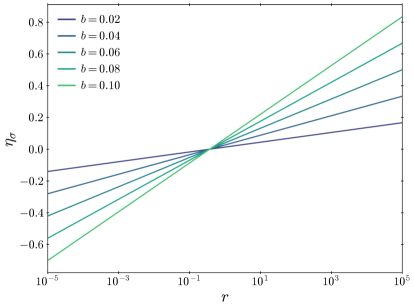
| (2.8) |
where is the field value normalized to the minimum . Fig. 1 shows the behavior of the eta parameter for across different values of . The results demonstrate that the quantum corrections drive to near the minimum, solving the eta problem. As we shall see in the next subsection, achieving the observed spectral index requires when the CMB scale exits the horizon during inflation. In fact, this condition can be naturally satisfied if the initial field value is . Since is a symmetry enhanced point, this initial condition can be explained by a positive mass for prior to observable inflation. Such a mass could arise either from a positive Hubble-induced mass around the origin or from a positive thermal mass.
The interactions responsible for the quantum corrections to the Hubble-induced mass term also generically renormalizes the self-quartic coupling of the spectator field. Although such corrections would ruin the flatness of the spectator field potential, these are suppressed in supersymmetric theories because of the non-renormalization of the superpotential [22, 23]. Consequently, our scenario is most effectively realized within supersymmetric theories. Supersymmetric theories also predict many light scalar fields, making it plausible for one of these fields to serve as the spectator field.
The flattening of the scalar potential by quantum corrections to the Hubble-induced mass term is noted in [24] for an inflaton potential. In fact, taking to be the inflaton field in Eq. (2.7), one may add a (nearly) constant potential term to drive inflation. However, such a setup generically suffers from fine-tuning problems. For , the potential becomes flat around the minimum of the potential, so inflation cannot end unless one introduces a waterfall field that couples to such that the waterfall field begins rolling around . Since is not a symmetry enhanced point, this requires the fine-tuning of parameters. On the other hand, for , the potential flattens around the maximum of the potential. For , the inflaton field rolls towards , and if a waterfall field is coupled to , the waterfalling at can end the inflation. However, this setup has an initial condition problem, as it must explain why the inflaton field is set around the maximum of the potential. Since the maximum of the potential is not a symmetry enhanced point, it is not possible to set the initial condition at the maximum through a positive thermal or Hubble-induced mass term. In [25], it is suggested that the initial condition may be set by tunneling from to whose rate is suppressed. For , the inflaton rolls toward larger field values, and the slow-roll condition may be violated around , ending the inflation. Nevertheless, the initial condition around still requires an explanation. In contrast, in our setup, the required initial condition of is around the origin, which can be naturally obtained as explained above.
2.2 Evolution of the spectral index
We now express the spectral index as a function of the model parameters. Using the expression for the potential given by Eq. (2.7), the spectral index as a function of the number of inflationary e-folds is
| (2.9) |
Using the equation of motion of in the slow-roll approximation,
| (2.10) |
and the parametrization of the potential in Eq. (2.8), the equation of motion of becomes
| (2.11) |
whose solution is
| (2.12) |
where is the initial normalized field value. Plugging this into Eq. (2.9), we find
| (2.13) |
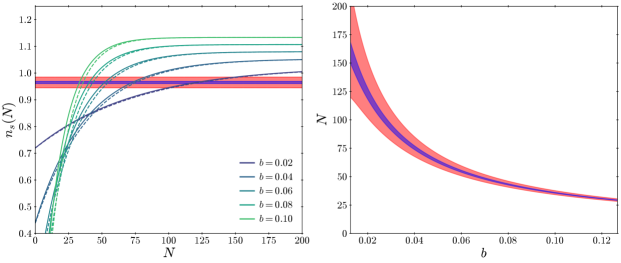
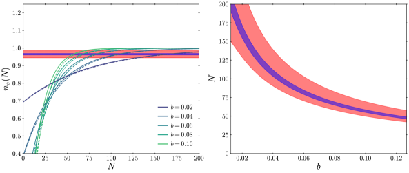
The left panel of Fig. 2 shows the spectral index as a function of the number of inflationary e-folds for different values of . While the classical initial condition set by the positive Hubble-induced mass or thermal mass is , we choose since quantum fluctuations introduce deviations of , where we used . The solid and dashed curves show where is computed analytically as in Eq. (2.12) using the slow-roll approximation and numerically without the approximation, respectively. Based on the agreement of the two curves, we adopt the slow-roll approximation in the following. The blue-shaded region marks areas where as measured by Planck at the confidence level. The red-shaded region highlights the extended range , which can be considered to be qualitatively similar to the observed one, since it describes a slightly red-tilted spectrum. This range can be used to qualitatively assess the naturalness of the model for a given value of .
The right panel of Fig. 2 shows the range of number of e-folds corresponding to the shaded regions in the left panel. For smaller values of , the field stays within these regions for a longer duration, indicating that the observed spectral index is likely a typical outcome of this model. One can see that for , the CMB scale should exit the horizon when after begins to roll from the origin. Typically, the number of e-folds after the CMB scale exits the horizon is . This means that the last inflation — the inflation accounting for the observed cosmic perturbations — should span a maximum total number of e-folds of . This, however, does not preclude the possibility of a longer total inflationary period, including an eternal one preceding the last inflation, provided that the spectator field remains trapped at the origin before the onset of the last inflationary phase.
We quantify the naturalness of the observed spectral index using the following fine-tuning measure introduced in [26] for the electroweak scale,
| (2.14) |
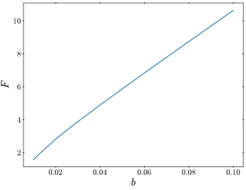
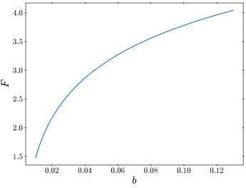
where quantifies the sensitivity of the observable to variations in a given model parameter . A large indicates that small changes in lead to large changes in , implying a high degree of fine-tuning. The overall fine-tuning measure is defined as the maximum sensitivity across all model parameters under consideration. Fig. 3 presents the dependence of this fine-tuning measure on the model parameter . For each value of , the parameter is chosen so that , with the initial field value set to . As shown in Fig. 3, when , , implying that more than fine-tuning is required to obtain the observed spectral index. In contrast, for , the required fine-tuning is negligible (), suggesting that the model operates naturally in this regime. However, it is important to note that requires an extended duration of the last inflation as shown in Fig. 2, which, depending on the specific inflation model, may require fine-tuning of the inflaton potential. The naturalness of the model should ultimately be assessed within the broader context of the entire inflationary scenario.
2.3 Running of the spectral index
One can also compute the running of the spectral index , which is defined as
| (2.15) |
where is the comoving wavenumber of a primordial mode and we have used that in the last equality. Using Eq. (2.11) yields
| (2.16) |
Using Eq. (2.9), we obtain
| (2.17) |
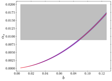
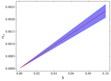
Fig. 4 shows the running computed at as a function of the parameter . The red curve shows the central value and the blue-shaded region shows the uncertainty of . The gray-shaded region in Fig. 4 is excluded by the Planck combined temperature and polarization data [27],
| (2.18) |
at the level, where we used the constraint from Planck and assumed that the uncertainty of is that of a Gaussian distribution. Future observations are expected to measure with a precision of [28, 29, 30]. From Figs. 3 and 4, one can see that our model can naturally explain the observed while producing an observable .
2.4 Non-Gaussianity
As mentioned earlier, our solution to the eta problem is applicable to generic spectator field models. In this subsection, we focus on a curvaton model with a quadratic vacuum potential, and compute the non-Gaussianity parameter as well as its correlation with the running of the spectral index.
We use the formalism [31, 32, 33] to derive the non-Gaussianity parameter. In this formalism, the curvature perturbation is computed as the difference in the number of e-folds among different patches in the universe, with the initial slice being a fixed flat slice, and the final slice being a uniform-density slice. Assuming that the curvaton energy density is negligible when it begins oscillation due to the vacuum potential, we can take the initial time slice to be when the curvaton begins to oscillate. Since the curvaton decays when its decay rate is around the expansion rate (which is determined by the total energy density of the universe), the time of curvaton decay also corresponds to a uniform-density slice.
The number of e-folds between the onset of curvaton oscillation and decay is given by
| (2.19) |
where and are the scale factors when the curvaton field starts to oscillate and decays, respectively. Since the curvaton energy density scales just like pressureless matter (),
| (2.20) |
where and are the curvaton energy densities at the onset of oscillation and just before decay, respectively, and is the curvaton field value when the oscillation begins. Furthermore, after the onset of curvaton oscillation, the curvaton energy density scales as while radiation energy density scales as , leading to
| (2.21) |
Since radiation dominates the energy density at the onset of oscillation, , where is the total energy density when the oscillation begins. Just before decay, the total energy density is given by . The curvaton energy density just before decay satisfies the following relationship,
| (2.22) |
Combining Eq. (2.20) with Eq. (2.22), we find
| (2.23) |
Assuming that the curvature perturbations generated by the curvaton field dominate, we can express up to the quadratic term in the field perturbation as
| (2.24) |
where the primes denote derivatives with respect to . The curvature perturbations can be split into a Gaussian (denoted by ) and a non-Gaussian part (denoted by ),
| (2.25) |
where is a Gaussian random field and describes the amplitude of the non-Gaussian correction. The non-Gaussianity is of the local type, meaning that only depends on the local value of the perturbations. From Eqs. (2.24) and (2.25), we deduce that
| (2.26) |
To find an expression for , we differentiate Eq. (2.23) with respect to , where (which is dominated by the radiation component) and (which is evaluated at a uniform-density slice) are independent of . Using the chain rule , we find
| (2.27) |
| (2.28) |
where the subscript denotes the derivative with respect to . Using Eq. (2.21),
| (2.29) |
where
| (2.30) |
and is the fractional curvaton energy density just before decay. If the curvaton energy density is sub-dominant, then the fluctuations in the curvaton energy density must be substantial to generate sufficiently large cosmic perturbations, which results in excessively large non-Gaussianity. Thus, in order to satisfy observational constraints coming from non-Gaussianity (refer to Eq. (2.38)), the curvaton must be the dominant component of the universe just before it decays. We therefore consider the limit where . In this limit, our expression for becomes [34]
| (2.31) |
We now compute as a function of , which is determined by the evolution of the curvaton field both during and after inflation. During inflation, the evolution is given by Eq. (2.12), and the field value at the end of inflation is given by
| (2.32) |
where is the number of e-folds at the end of inflation. After inflation, the inflaton field begins to oscillate around the minimum and behaves as matter. During this period, the Hubble-induced mass of is generically different from that during inflation and is given by
| (2.33) |
where and are constants. As we show in Appendix A, for one-field supersymmetric inflation models, and . In more generic models, and may take different values. Solving the equation of motion in Appendix B, we find
| (2.34) |
where we assumed and is a constant independent of . The evolution of by the Hubble-induced mass term ceases when either the vacuum potential of dominates over the Hubble-induced mass, after which begins to oscillate, or when reheating ends, after which the Hubble-induced mass becomes negligible. Denoting the number of e-folds at which this occurs as , is given by
| (2.35) |
Using Eqs. (2.26) and (2.35), we obtain
| (2.36) |
where parametrizes the duration of the non-harmonic curvaton evolution after horizon exit. Eq. (2.36) shows that suppresses the effect of the curvaton’s post-inflationary dynamics on non-Gaussianity. Additionally, a positive value of enhances the curvaton field value helping the curvaton dominate the universe [35].
The contribution to during inflation is typically , while post-inflationary dynamics, specifically during matter-domination, contribute an additional term
| (2.37) |
where is the Hubble scale at , is the Hubble scale during inflation ( GeV)222 If GeV, must be around the Planck scale to explain . This means that the Hubble-induced mass must be as small as at the UV scale. To obtain the small Hubble-induced mass by its running rather than by a UV boundary condition, it is preferable that GeV. , and is bounded below by the soft mass scale ( TeV). In supersymmetric one-field inflation models, and . For these parameters, is at most 17, and smaller values of the inflation scale or larger curvaton masses reduce this contribution further. As a result, the total typically falls in the range .
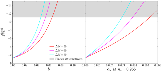
The left panel of Fig. 5 shows as a function of for different values of . As increases, the curvaton potential becomes less harmonic, leading to a corresponding increase in . Observational constraints on local non-Gaussianity, derived from the combined temperature and polarization Planck data, impose the following bound [36]
| (2.38) |
at the level, where we used the constraint from Planck and assumed that the uncertainty is that of a Gaussian distribution. The gray-shaded region in Fig. 5 represents the parameter space excluded at the level.
Eqs. (2.17) and (2.36) can be used to derive the following correlation between the local non-Gaussianity parameter and the running of the spectral index,
| (2.39) |
This relationship, evaluated at , is depicted in the right panel of Fig. 5. Allowing for the uncertainty in the precise value of , Eq. (2.39) establishes a relation between and within a few ten percents. Upcoming cosmological probes targeting non-Gaussianity and the running [29] offer a direct opportunity to test this prediction.
3 Spectator field models with approximate symmetry
In this section, we consider a scenario with a complex scalar field , which can be decomposed into a radial component and an angular component ,
| (3.1) |
We assume to possess an approximate symmetry, which guarantees that the Hubble-induced mass of is suppressed. As a result, if the cosmic perturbations are sourced by the fluctuations of , the eta problem can be avoided [21]. However, an important question remains: why does the spectral index deviate from unity by ? The scenario described below, which utilizes quantum corrections to the Hubble-induced mass of , can naturally explain this deviation.
3.1 Evolution of the spectral index
During inflation, the radial direction obtains a Hubble-induced mass and rolls along the potential in Eq. (2.7) while obtaining fluctuations. The angular direction , owing to the approximate symmetry, remains nearly massless and is frozen up to fluctuations produced during inflation. After inflation, the radial direction is relaxed to the minimum of the potential with and its fluctuations are dampened.333 If the fluctuations of the radial direction are not dampened, then both the angular and radial fluctuations contribute to the cosmic perturbations, resulting in a spectral index that falls between the values shown in Figs. 2 and 6. For this to occur, the potential of after inflation should not be dominated by the potential in Eq. (2.7), where the mass of around the minimum is small and the radial direction is not dampened. Instead, the dominant part of the potential should be the vacuum wine-bottle potential or one with an unsuppressed negative Hubble-induced mass term stabilized by a positive vacuum potential. The mass of the angular direction is assumed to be still negligible and its fluctuations are frozen on super-horizon scales. Eventually, the mass of the angular direction arising from explicit breaking becomes comparable to the Hubble scale and the fluctuations in the angular direction are converted into fluctuations in the energy density of . This may occur as oscillations in the angular direction with fixed [21], or as a spiral motion of in field space [37, 38, 39, 40] by the Affleck-Dine mechanism [41]. The spiral motion, if the angular momentum is sufficiently large, is naturally long-lived because of the approximate charge conservation [42, 43] and naturally dominates the universe, making it a good curvaton candidate [40]. Also, the charge can be converted into baryon asymmetry without producing baryon isocurvature perturbations [40].
In the above setup, the angular direction is the spectator field, and hence its fluctuations are responsible for the cosmic perturbations, . The dynamics of the radial direction indirectly affects the spectrum of the fluctuations of the angular direction, which is given by
| (3.2) |
The spectrum of curvature perturbations is
| (3.3) |
Then, the spectral index is given by
| (3.4) |
Using Eq. (2.12), we obtain
| (3.5) |
The left panel of Fig. 6 shows the spectral index as a function of the number of e-folds for different values of , with . In this model, is smaller than since the radial direction stops evolving at the minimum of the potential. The blue-shaded region shows the areas with as measured by Planck at the confidence level, while the red-shaded region indicates where . The right panel of Fig. 6 shows the number of e-folds corresponding to the shaded regions in the left panel. Compared to the model presented in Sec. 2, the number of e-folds between when the spectator field begins to roll from the origin and when the CMB scale exits the horizon needs to be larger. The red-shaded regions are wider than those in Fig. 2, indicating that the observed spectral index can be achieved more naturally in this setup.
3.2 Running of the spectral index
The running of the spectral index is
| (3.6) |
which is shown in Fig. 8. The red curve shows at and the blue-shaded region shows that for . An observable value of the running () can be produced for while naturally explaining the observed spectral index .
4 Summary
In this work, we propose a spectator field scenario where quantum corrections to the scalar potential address the eta problem while simultaneously explaining the slight deviation of cosmic perturbations from scale-invariance. We demonstrate that these quantum corrections induce an attractor behavior during inflation, driving the spectator field toward a region in field space where the curvature perturbations are nearly scale-invariant. If the initial condition of the spectator field is set at the origin of the field space, the resulting spectrum of curvature perturbations can be slightly red-tilted. We further evaluate the naturalness of the observed spectral index by employing a fine-tuning measure and demonstrate that the observed spectral index can be obtained naturally within our model. Also, we show that an observable value of the running of the spectral index can be produced in a parameter region without fine-tuning.
Spectator field models generically predict large non-Gaussianity of the cosmic perturbations. We focus our analysis on a curvaton model with a quadratic vacuum potential and compute the primordial non-Gaussianity and running of the scalar spectral index. We derive a relationship between these two cosmological observables, providing an important theoretical prediction of the model that is testable with the next-generation cosmological probes.
We further demonstrate the versatility of our approach by applying it to a broader class of models where the angular direction of a complex scalar field with an approximate symmetry serves as the spectator field. Using the fine-tuning measure, we find that the observed spectral index can be obtained naturally also in this model by the attractor behavior of the radial direction of the complex scalar field, while possibly producing an observable value of the running.
Acknowledgments
We thank Aaron Pierce for commenting on the draft. K.H. is supported by the Department of Energy under Grant No. DE-SC0025242, a Grant-in-Aid for Scientific Research from the Ministry of Education, Culture, Sports, Science, and Technology (MEXT), Japan (20H01895), and by World Premier International Research Center Initiative (WPI), MEXT, Japan (Kavli IPMU).
Appendix A Hubble-induced mass after inflation
In this appendix, we derive the relation between the Hubble-induced masses of the spectator field during and after inflation in supersymmetric one-field inflation models. In particular, we show that in these models, the coefficient matches and the Hubble-induced mass after inflation drives the spectator field to larger field values.
The inflaton field and the spectator field are embedded into chiral multiplets and , respectively. Their Kahler potential is given by
| (A.1) |
where is a function that encodes the tree and quantum level coupling between and . Taking the reduced Planck scale to be unity, the potential of and is
| (A.2) |
where we assumed , and the inflaton potential is determined by the superpotential of . By matching this potential with Eq. (2.7) using during inflation, we obtain
| (A.3) |
The kinetic term of the inflaton is given by
| (A.4) |
After inflation, the Hubble-induced potential of becomes
| (A.5) |
where we used . Comparing Eq. (A.5) with Eq. (2.33), one can see that and the spectator field obtains an extra negative Hubble-induced mass with a coefficient , which drives the field to larger field values.
Appendix B Dynamics during matter domination
In this appendix, we solve the equation of motion of during the matter dominated era after inflation. The potential of can be parameterized as
| (B.1) |
Then, the equation of motion of is given by
| (B.2) |
Taking the number of e-folds as the time variable, the equation of motion becomes
| (B.3) |
We denote the solution for by , which is given by
| (B.4) |
where , , and we assumed . In the last equality, we neglect the second term in Eq. (B.4) since it decays faster than the other term. Defining by , the equation of motion of is given by
| (B.5) |
Under the slow-roll approximation for (), we find the evolution of is governed by
| (B.6) |
which can be solved as
| (B.7) |
where is a constant that is independent of . The solution for is then
| (B.8) |
where is another constant also independent of . Using this formula, we may derive the prediction on the local non-Gaussianity, as shown in Sec. 2.
References
- [1] V.F. Mukhanov and G.V. Chibisov, Quantum Fluctuations and a Nonsingular Universe, JETP Lett. 33 (1981) 532.
- [2] S.W. Hawking, The Development of Irregularities in a Single Bubble Inflationary Universe, Phys. Lett. B 115 (1982) 295.
- [3] A.A. Starobinsky, Dynamics of Phase Transition in the New Inflationary Universe Scenario and Generation of Perturbations, Phys. Lett. B 117 (1982) 175.
- [4] A.H. Guth and S.Y. Pi, Fluctuations in the New Inflationary Universe, Phys. Rev. Lett. 49 (1982) 1110.
- [5] J.M. Bardeen, P.J. Steinhardt and M.S. Turner, Spontaneous Creation of Almost Scale - Free Density Perturbations in an Inflationary Universe, Phys. Rev. D 28 (1983) 679.
- [6] S. Mollerach, Isocurvature Baryon Perturbations and Inflation, Phys. Rev. D 42 (1990) 313.
- [7] A.D. Linde and V.F. Mukhanov, Nongaussian isocurvature perturbations from inflation, Phys. Rev. D 56 (1997) R535 [astro-ph/9610219].
- [8] K. Enqvist and M.S. Sloth, Adiabatic CMB perturbations in pre - big bang string cosmology, Nucl. Phys. B 626 (2002) 395 [hep-ph/0109214].
- [9] D.H. Lyth and D. Wands, Generating the curvature perturbation without an inflaton, Phys. Lett. B 524 (2002) 5 [hep-ph/0110002].
- [10] G. Dvali, A. Gruzinov and M. Zaldarriaga, A new mechanism for generating density perturbations from inflation, Phys. Rev. D 69 (2004) 023505 [astro-ph/0303591].
- [11] L. Kofman, Probing string theory with modulated cosmological fluctuations, astro-ph/0303614.
- [12] T. Moroi, T. Takahashi and Y. Toyoda, Relaxing constraints on inflation models with curvaton, Phys. Rev. D 72 (2005) 023502 [hep-ph/0501007].
- [13] A.D. Linde, Chaotic Inflation, Phys. Lett. B 129 (1983) 177.
- [14] K. Freese, J.A. Frieman and A.V. Olinto, Natural inflation with pseudo - Nambu-Goldstone bosons, Phys. Rev. Lett. 65 (1990) 3233.
- [15] E.J. Copeland, A.R. Liddle, D.H. Lyth, E.D. Stewart and D. Wands, False vacuum inflation with Einstein gravity, Phys. Rev. D 49 (1994) 6410 [astro-ph/9401011].
- [16] A. Vilenkin, Predictions from quantum cosmology, Phys. Rev. Lett. 74 (1995) 846 [gr-qc/9406010].
- [17] M. Tegmark, What does inflation really predict?, JCAP 04 (2005) 001 [astro-ph/0410281].
- [18] B. Freivogel, M. Kleban, M. Rodriguez Martinez and L. Susskind, Observational consequences of a landscape, JHEP 03 (2006) 039 [hep-th/0505232].
- [19] Planck collaboration, Planck 2018 results. VI. Cosmological parameters, Astron. Astrophys. 641 (2020) A6 [1807.06209].
- [20] D.H. Lyth and A.R. Liddle, The primordial density perturbation: Cosmology, inflation and the origin of structure (2009).
- [21] K. Dimopoulos, D.H. Lyth, A. Notari and A. Riotto, The Curvaton as a pseudoNambu-Goldstone boson, JHEP 07 (2003) 053 [hep-ph/0304050].
- [22] M.T. Grisaru, W. Siegel and M. Rocek, Improved Methods for Supergraphs, Nucl. Phys. B 159 (1979) 429.
- [23] N. Seiberg, Naturalness versus supersymmetric nonrenormalization theorems, Phys. Lett. B 318 (1993) 469 [hep-ph/9309335].
- [24] E.D. Stewart, Flattening the inflaton’s potential with quantum corrections, Phys. Lett. B 391 (1997) 34 [hep-ph/9606241].
- [25] E.D. Stewart, Flattening the inflaton’s potential with quantum corrections. 2., Phys. Rev. D 56 (1997) 2019 [hep-ph/9703232].
- [26] R. Barbieri and G.F. Giudice, Upper Bounds on Supersymmetric Particle Masses, Nucl. Phys. B 306 (1988) 63.
- [27] Planck collaboration, Planck 2018 results. X. Constraints on inflation, Astron. Astrophys. 641 (2020) A10 [1807.06211].
- [28] K. Kohri, Y. Oyama, T. Sekiguchi and T. Takahashi, Precise Measurements of Primordial Power Spectrum with 21 cm Fluctuations, JCAP 10 (2013) 065 [1303.1688].
- [29] SPHEREx collaboration, Cosmology with the SPHEREX All-Sky Spectral Survey, 1412.4872.
- [30] X. Li, N. Weaverdyck, S. Adhikari, D. Huterer, J. Muir and H.-Y. Wu, The Quest for the Inflationary Spectral Runnings in the Presence of Systematic Errors, Astrophys. J. 862 (2018) 137 [1806.02515].
- [31] M. Sasaki and E.D. Stewart, A General analytic formula for the spectral index of the density perturbations produced during inflation, Prog. Theor. Phys. 95 (1996) 71 [astro-ph/9507001].
- [32] D. Wands, K.A. Malik, D.H. Lyth and A.R. Liddle, A New approach to the evolution of cosmological perturbations on large scales, Phys. Rev. D 62 (2000) 043527 [astro-ph/0003278].
- [33] D.H. Lyth, K.A. Malik and M. Sasaki, A General proof of the conservation of the curvature perturbation, JCAP 05 (2005) 004 [astro-ph/0411220].
- [34] M. Sasaki, J. Valiviita and D. Wands, Non-Gaussianity of the primordial perturbation in the curvaton model, Phys. Rev. D 74 (2006) 103003 [astro-ph/0607627].
- [35] T. Fujita and K. Harigaya, Hubble induced mass after inflation in spectator field models, JCAP 12 (2016) 014 [1607.07058].
- [36] Planck collaboration, Planck 2018 results. IX. Constraints on primordial non-Gaussianity, Astron. Astrophys. 641 (2020) A9 [1905.05697].
- [37] J. McDonald, Supersymmetric curvatons and phase induced curvaton fluctuations, Phys. Rev. D 69 (2004) 103511 [hep-ph/0310126].
- [38] A. Riotto and F. Riva, Curvature Perturbation from Supersymmetric Flat Directions, Phys. Lett. B 670 (2008) 169 [0806.3382].
- [39] K. Harigaya and M. Yamada, Cosmic perturbations, baryon asymmetry and dark matter from the minimal supersymmetric standard model, Phys. Rev. D 102 (2020) 121301 [1907.07687].
- [40] R.T. Co, K. Harigaya and A. Pierce, Cosmic perturbations from a rotating field, JCAP 10 (2022) 037 [2202.01785].
- [41] I. Affleck and M. Dine, A New Mechanism for Baryogenesis, Nucl. Phys. B 249 (1985) 361.
- [42] R.T. Co and K. Harigaya, Axiogenesis, Phys. Rev. Lett. 124 (2020) 111602 [1910.02080].
- [43] V. Domcke, K. Harigaya and K. Mukaida, Charge transfer between rotating complex scalar fields, JHEP 08 (2022) 234 [2205.00942].