Dynamical system analysis of Bianchi III Universe with gravity theory
Abstract
Bianchi type III (BIII) metric is an interesting anisotropic model to study cosmic anisotropy as it has an additional exponential term multiplied by a directional scale factor and recasting the cosmological model as a dynamical system to provide various significant information regarding the evolution, stability of the system, etc. Here in this work, we have considered the BIII metric under the framework of gravity theory and studied the dynamical system analysis for three different models. It is found that the first two models i.e. and are consistent with standard CDM cosmology but the third one i.e. have some issue of physical viability. Thus we can remark that some models may not be suitable for studying the evolution of the Universe with an anisotropic background like using BIII metric etc. However, all three models agree with the heteroclinically connected path of radiation, matter, and dark energy dominated phases of the Universe as predicted by standard cosmology.
I Introduction
Homogeneity and isotropy are the two basic cosmological principles that form the basis of standard cosmology, often known as the CDM cosmology. This cosmological model provides answers to many questions about our understanding of the world through the Friedmann-Lemaître-Robertson-Walker (FLRW) metric, together with the energy-momentum tensor in the conventional perfect fluid form [1]. Researchers are encouraged to expand this traditional formalism to identify alternative theories or modifications to general relativity (GR) for a number of reasons, including the Universe’s current rapid expansion [2, 3, 4], non-observational evidence about dark matter (DM) [5], and dark energy (DE) [6]. Therefore, a good number of modified formalisms of GR have been developed to refute the idea of the Universe’s exotic matter and energy contents used to describe respectively its missing mass and current rapid expansion, usually referred to as the modified theories of gravity (MTGs).
The most basic MTG is the theory of gravity [7, 8, 9], which substitutes a function of the Ricci scalar for the Ricci scalar in the Einstein-Hilbert action of GR. This theory shows its versatility in cosmology, black hole physics [10, 11, 12, 13, 14], cosmic ray physics [15, 16], and other theoretical research fields [17, 19, 18]. The Refs. [20, 21, 22, 23, 24] contain a comprehensive collection of cosmological studies for both isotropic and anisotropic Universes using the theory of gravity. The gravity [9, 25], in which the gravitational Lagrangian density is the arbitrary function of both the Ricci scalar and the trace of the energy-momentum tensor , is another well-liked MTG in cosmology as well as other areas of gravitational physics and related domains. The source term that represents the change in the energy-momentum tensor with respect to the metric is the foundation of the theory. The matter Lagrangian density serves as the basis for the general formulation of this source term. The field equations generated by each option are distinct [26, 27, 28]. Numerous studies have been conducted using the theory of gravity, some may be found in Refs. [25, 29, 30, 31, 32, 33]. In addition to these MTGs, some other theories, such as teleparallel gravity theories, like gravity theory [34, 35, 36, 37, 38], gravity theory [39, 40, 42, 41, 43, 44, 45], and some standard model extension (SME) like bumblebee gravity theory [46, 47, 48], which are usually termed together as the alternative theories of gravity (ATGs), have gained popularity among cosmological scholars in recent years. Comparison of these MTGs and ATGs to data has yielded encouraging results [26, 33, 38, 48, 45].
There are several shortcomings when taking into account common assumptions like isotropy and homogeneity in cosmological research, in addition to the absence of direct empirical proof of the existence of exotic matter and energy contents as mentioned. Despite these presumptions, researchers have been able to explain the majority of cosmological aspects using the standard CDM model, which includes the Hubble tension [49, 50], the tension [49], the coincidence problem [51], and others. Nonetheless, many reliable observational data sources, such as WMAP [52, 53, 54], SDSS (BAO) [55, 56, 57], and Planck [58, 49], have revealed some departures from the conventional cosmological principles and raise the possibility that the Universe contains some anisotropies. Additionally, studies indicate that the Universe’s shape is large-scale planar symmetric. Without changing the higher-order multipole of temperature anisotropy in the CMB angular power spectrum, the eccentricity of order can match the quadrupole amplitude with observational evidence [59]. The existence of asymmetry axes in the Universe is confirmed by polarization studies of electromagnetic radiation traveling great distances [60]. Thus, not all cosmic features can be adequately explained by the principles of homogeneity and isotropy alone.
A metric with a homogeneous background and an anisotropic feature is required to describe the anisotropic nature of the Universe. In order to extract anisotropy information for cosmological investigations, researchers often choose Bianchi types I, III, V and IX, which are among the eleven types of anisotropic metrics that Luigi Bianchi suggested [61]. The majority of the cosmological studies in these metrics are mostly confined to type I, and relatively little research has been done in this area. Some works on anisotropic cosmological investigations in Bianchi type I metric can be found in Refs. [62, 63, 64, 65, 66, 67, 68, 69, 70]. However, as mentioned already the study in Bianchi type III (BIII) metric is very much limited. A few works in the BIII metric are mentioned here as follows. A. Moussiaux et al. in 1981 had found an exact particular solution to the Einstein field equations for the vacuum which includes a cosmological constant in the BIII metric [71]. D. Lorenz put up a model that incorporates dust and a cosmological constant in the BIII metric in 1982 [72]. Ref. [73] has made another study that suggested a viscous cosmological model with the variable and gravitational constant . J. P. Singh et al. had examined a work with the variable and in the presence of a perfect fluid, assuming a conservation rule for the energy-momentum tensor in the BIII metric in 2007 [74]. In Ref. [75], a BIII model with a perfect fluid, the time-dependent , and constant deceleration parameter were discovered. P. S. Letelier in 1980 had studied certain two-fluid cosmological models that have symmetries similar to those of the BIII models. In these models, an axially symmetric anisotropic pressure is produced by the independent four-velocity vectors of the two non-interacting perfect fluids [76].
In our work, we try to study the BIII Universe as a dynamical system to understand its evolution and the possibility of various phases of it. Dynamical system analysis is a powerful and elegant way to study the dynamics of the Universe through recasting the cosmological equations as a dynamical system [77]. The dynamical system technique has been used to investigate the stability of systems employing a variety of cosmological models, including the canonical [78, 79] and non-canonical scalar-field models [80, 81, 82], the scalar-tensor theories [83, 84], the gravity theory [85, 86, 87], and others [88, 89, 90, 91]. Ref. [92] provides a contemporary overview of the dynamical system method. A study on dynamical system analysis of isotropic Universe in theory has been found in Ref. [93]. The cosmic dynamical system in gravity theory has also been the subject of a few studies [94, 95]. However, there aren’t many comparable studies using the Bianchi metric in the theory. Thus we intend to investigate it using the BIII metric to learn more about the anisotropic Universe in gravity theory. Here we are considering the BIII metric in gravity theory to understand the Universe as a dynamical system. In this work, we are using constrained values of various cosmological parameters from Ref. [96] which are constrained through various observational data like Hubble data, Pantheon plus data, BAO data, etc. through powerful the Bayesian inference technique, and plot the phase portraits of dynamical variables to understand the evolution of the Universe for different gravity models.
The current article is organized as follows. Starting from the introduction part in Section I to explain the importance of the BIII Universe and MTGs, specifically the gravity theory from various litterateurs, we discuss the general form of field equations in gravity theory in Section II. In Section III, we develop the required field equations and continuity equation for the BIII metric for two different models. In Section IV, the dynamical system analyses for two different models have been performed. In Section V we study a special model and test its physical viability. Finally, the article has been summarized with conclusions in Section VI.
II gravity theory and field equations
For the theory of gravity, the modified Einstein-Hilbert action may be expressed as [25]
| (1) |
where . The field equations for the theory can be obtained by varying the action (1) with respect to the metric tensor and can be written as
| (2) |
where and are the derivatives of with respect to Ricci scalar and trace of the energy-momentum tensor respectively, and the energy-momentum tensor can be written as
| (3) |
The tensor term can be expressed as [25]
| (4) |
For the conventional diagonal energy-momentum tensor, the matter Lagrangian can be considered as [25]. Thus, the reduces to
| (5) |
With the help of the general form of field equations (2), we derive field equations for the BIII metric for the conventional perfect fluid in the next sections for some specific gravity models.
III Bianchi III Cosmology in gravity Theory
The BIII metric in our study has the form:
| (6) |
Here, , and are the directional scale factors along , and directions respectively and is a constant. Thus, we have three directional Hubble parameters , and along , and directions respectively. The average scale factor for the metric is and the average Hubble parameter can be written as
| (7) |
In our work, we consider the conventional perfect fluid model of the Universe and for this model the energy-momentum tensor , and hence the components of from equation (5) can be obtained as , , , and . We are now in a position to derive field equations for the gravity models under consideration in the BIII metric. We consider the following two forms of models in our study as suggested in Ref. [25]:
| (8) |
With these two forms of models, we proceed as follows.
III.1
This is a standard form of the gravity model. In our study, we consider the explicit form of this model as . Here and are two free model parameters. The metric-independent form of the field equations for the considered model can be written as
| (9) |
For the BIII metric with in which is a constant, along with the considered conventional energy-momentum tensor, the set of field equations from equation (9) has been derived as
| (10) |
| (11) | ||||
| (12) | ||||
| (13) | ||||
| (14) |
We observe from equation (14) that there are few possibilities regarding the parameter and the directional Hubble’s parameters. For and along with the consideration of , we can rewrite the above-mentioned field equations as
| (15) | |||
| (16) | |||
| (17) |
On the other hand, for the condition , equations (10), (11), (12) and (13) can be rewritten as
| (18) | |||
| (19) | |||
| (20) | |||
| (21) |
Further, for the condition of and , those field equations now can be rewritten as
| (22) | |||
| (23) | |||
| (24) |
From the metric equation (6) one can observe that for the metric reduces from BIII Universe to LRS-BI Universe, and for it reduces to standard BI Universe. As our prime objective is to carry out this work to explore the BIII Universe, thus we are only interested in looking at the case in our study. The shear scalar for the considered case can be written as
| (25) |
III.1.1 Cosmological parameters for case
For and , we have already derived the field equations as given equations (15), (16) and (17). Now further considering through using the condition in which and are the expansion scalar and shear scalar respectively, we can rewrite the field equations as
| (26) | |||
| (27) |
Moreover, the continuity equation for considered can be obtained by using the condition as
| (28) |
The above equation shows that despite taking into account the BIII metric, the energy conservation condition remains identical to that of standard isotropic cosmology and thus the anisotropy affects only the geometry of the spacetime. Now, using equations (26) and (27) we can obtain the effective equation of state and it takes the form:
| (29) |
Accordingly the deceleration parameter can be written as
| (30) |
Again, using the relation in which is the equation of state with for matter, for radiation and for dark energy, the solution for from the continuity equation (28) can be obtained as
| (31) |
Now, the required set of equations for cosmological parameters is ready for further analysis. One of the major tasks from here is to constrain the different cosmological and model parameters that appear in different cosmological expressions. The detailed methods of parameter constraining have been discussed in later sections.
III.2
This model is the simplified version of the previous model with , and . Thus the field equations for this considered model can be written for , and as
| (32) | |||
| (33) |
Consequently, the expressions of the effective equation of state () and the deceleration parameter () for this model can be derived from equations (29) and (30) respectively.
IV Dynamical system analysis of the BIII metric in models
In this section, we analyse the BIII Universe as a dynamical system by using the above mentioned gravity models. Here we try to assess the system stability by identifying the critical points and their characteristics.
IV.1 Model
Using dynamical variables the Friedmann equation (26) for this model can be expressed in the form:
| (34) |
where , , and are the dynamical variables with , and as the densities of matter, radiation and dark energy respectively. , and are basically the matter density parameter , radiation density parameter and dark energy density parameter respectively. Further, we can rewrite the equation (27) by considering the dynamical variables and equation (34) as
| (35) |
Again, the derivatives of and with respect to take the forms:
| (36) | |||
| (37) |
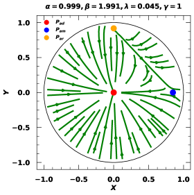
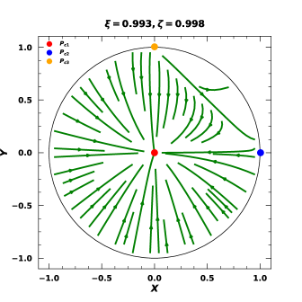
The effective equation of state and the deceleration parameters can be calculated from equations (29) and (30) respectively. With the help of the dynamical system equations ((36) and (37)) we accomplished the fixed point analysis and the results are compiled in Table 1 and the phase space portraits of versus are shown for both the and CDM models in Fig. 1. In this analysis, we have used the constrained values of all the model parameters from Ref. [96], where these parameters are constrained by using various observational cosmological data sources through employing powerful Bayesian techniques.
| Model | Fixed point | Eigenvalues | ||||
|---|---|---|---|---|---|---|
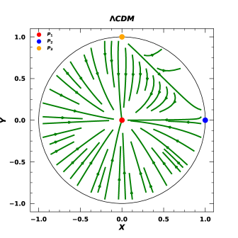
The phase space portraits in Fig. 1 show the critical points indicating different phases of the BIII Universe in the model along with the CDM cosmological results. The phase portrait of our model is similar to the standard isotropic cosmology which predicts the radiation-dominated, matter-dominated and dark energy-dominated phases and they are hetero clinically connected. However, there are some subtle differences that have been observed in both the plots too. The critical points for the BIII Universe are shifted to a less than unity state in contrast to the CDM plot. These shifts occur due to imposition of directional anisotropy in the BIII Universe. However, the track of the evolution of the Universe is intact as predicted by the standard cosmology which means that there are radiation-dominated, matter-dominated, and dark energy-dominated phases but in BIII Universe this evolution track is influenced by an anisotropic effect. Further, from Table 1 we have observed that the for the matter-dominated phase (i.e. point ) is non-zero but a very small negative value which may indicate a minute presence of dark energy influence in that phase. From the table, we also observed that the value as the Friedmann equation is modified as equation (34). This value of density can be interpreted as the shear energy stored in the form of spacetime deformation due to the presence of directional anisotropy with some model effect.
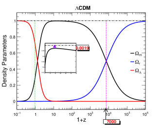
The evolution of density parameters against the cosmological redshift for the considered model with the constrained values of the model parameters has also been studied and compared with the standard CDM results in Fig. 2. From the plots, one can find that there are no pure radiation, matter, or dark energy phases as we found them in the standard CDM results but shows the dominance of radiation or matter or dark energy in those phases in BIII Universe as the density parameters never reached unity. The gap between the maximum value of any density parameters from unity is mainly due to the presence of anisotropy along with the considered specific model. The anisotropy causes deformation in the spacetime leading to shear energy storing in the spacetime fabric which contributes to the total density of the Universe. Apart from that there is a shift in the value of from the standard CDM results in BIII Universe for the considered model at which the matter-dominated phase had started dominating over the radiation-dominated phase. This shift is again due to the contribution of anisotropy and the effect of the model. Thus, we can remark that anisotropy may influence the evolutionary track of the BIII Universe.
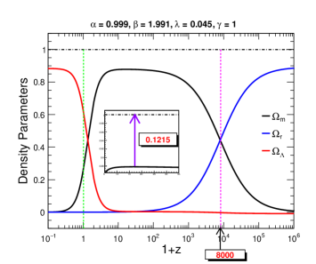
However, to quantify the effect of the model in the BIII Universe evolution, we have further tested the density parameter evolution and phase space portrait for the considered model by setting the , which is nothing but the isotropic case and the results are shown in Fig. 3. From the figure we have found that there is not much difference in the density parameter plot from Fig. 2. There is only a slight difference in the gap from the unity to the maximum value of as seen from Fig. 2 and Fig. 3, which is around and this difference is mainly due to the absence of anisotropy. Hence we can make a comment that anisotropy has a very minimal role in evolution although it is not zero. Further, the transition point between radiation-dominated and matter-dominated is the same for both isotropic and anisotropic cases, hence no role of anisotropy on the shift of the transition point from standard CDM plot. Thus this shift of transition point seen in Fig. 2 is purely a model effect. Apart from that, the phase space portraits of Fig. 1 (right) and Fig. 3 (right) are almost similar while following the heteroclinic path. Nevertheless, the critical points in the isotropic case are which are slightly different from the anisotropic case (). In the anisotropic case, we have observed that the critical points are . With these observations, we can say that the model effect has a more dominant role in the evolution as compared to anisotropy.
IV.2 Model
The Friedmann like equation for the considered model with can be written from the equation (32) as
| (38) |
Here, the variables and are the same as in the previous model. Similarly, we can rewrite equation (33) in terms of these dynamical variables as
| (39) |
Now we can obtain the dynamical system equations i.e. the derivative of and with respect to which takes the form:
| (40) | |||
| (41) |
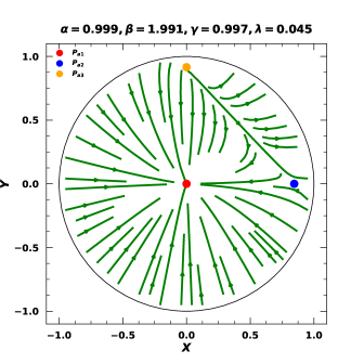
The effective equation of state and deceleration parameters can be derived from equations (29) and (30) respectively as we did for the previous model. From equation (40) and (41) we analyse the critical points for this considered model and results are compiled in Table 2. Further, we plot the phase portrait of versus for the model which has been shown in Fig. 4. As in the previous case for this plot also we consider the constrained values of model parameters from Ref. [96].
| Model | Fixed point | Eigenvalues | ||||
|---|---|---|---|---|---|---|
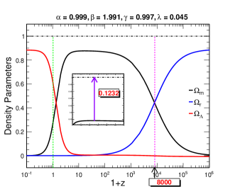
From Fig. 4 and Table 2 like in the previous model we can observe the shift of critical points from the standard CDM model for this model too. As we have previously claimed, the anisotropy has the role of shifting these points from the unity value in this model also. Further, there is a very small negative value of observed in the matter-dominated phase which indicates a very small role of dark energy in the matter-dominated phase of the evolution in the BIII type of Universe. Apart from that, we observe a similar hetero clinic sequence of evolution of the BIII Universe like standard cosmology i.e. Universe evolved from radiation-dominated to matter-dominated and then to dark energy-dominated phase (). Moreover, like in the previous model analysis we see that , and this non-zero contribution is due to the presence of anisotropy and the effect of the model which we have already discussed in our previous model. The presence of these effects can be observed in all three phases. Thus a prominent role of model and a minimal role of anisotropy is present in the entire evolution of the Universe as claimed in the previous model analysis. As in the case of the previous model, we also study the evolution of the density parameters with cosmological redshift in this model which has been shown in Fig. 5. The model shows almost similar results as in the previous case and clearly indicates the influence of the model and the anisotropy in the evolution of the Universe.
V A special case
In this section, we are interested in studying a special model which shows inconsistency with the standard cosmological evolution as predicted by CDM model [96]. The field equations for the considered model can be written as [96]
| (42) | |||
| (43) |
Here are model parameters, and is the directional anisotropy parameter ( in previous models). The Friedmann-like equation can be obtained from equation (42) and it takes the form:
| (44) |
Again, from equation (43) we can obtain
| (45) |
With the help of equation (44) and (45) we construct the dynamical system equations as
| (46) | |||
| (47) |
Both equations (46) and (47) are not only dependent on dynamical variables and like previously mentioned models but also depend on other variables like Ricci scalar and the trace of the energy-momentum tensor which themselves are the functions of and . Thus, the situations are more complicated in this model. However, from Ref. [96] we found that the constrained values of and are very small and hence we can write , and . With these approximations, we can rewrite the equation (46) and (47) as
| (48) | |||
| (49) |
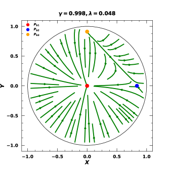
We have compiled the fixed-point solutions for the considered model in Table 3 and drawn the phase portrait for versus for the constrained set of model parameters from Ref. [96] in Fig. 6. and in this table are obtained by using equations (29) and (30) respectively with replacing by as directional anisotropic parameter.
| Model | Fixed point | Eigenvalues | ||||
|---|---|---|---|---|---|---|
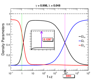
From Table 3, it is found that there are three critical points and corresponding to three different phases of the Universe: dark energy, matter, and radiation era as predicted by standard cosmology, and the phase portrait in Fig. 6 shows the hetero clinic transition from which is again predicted by the standard cosmology. However, if we insert the constrained values of and from Ref. [96] then the values of and are found to be close to CDM model values (Table 4). In both the table 3 and 4, refers to the sum of the contribution of and the anisotropic effect due to . However, for the matter-dominated phase (i.e. ) the values of and are highly negative, which is not match with standard cosmology and thus it further supports the claim of non-suitability of this model to study matter-dominated phase as claimed by Ref. [96]. Apart from that, the values of and in matter and radiation-dominated phases are and respectively, which are slightly greater than unity that violates the total density equal to one and thus raises the question of the physical viability of the model. Therefore even though the model predicts the standard cosmological transition path as predicted by the CDM model, its results are not physically viable and thus the model is not suitable for cosmological study in the BIII Universe.
| Model | Fixed point | Eigenvalues | ||||
|---|---|---|---|---|---|---|
Since in the first two models, we have observed that the model has the more dominant role than anisotropy and thus, the absurdity in the results observed in this special case is also may be due to the model and hence further strengthens our claim of non-suitability of the considered model. As the results are not physically viable hence we have to restrict ourselves from further studies on this model.
VI Conclusions
In this paper, we have considered the BIII Universe in gravity theory with three different models to study the Universe as a dynamical system and checked the stability through critical point analysis, and also tried to understand the influence of anisotropy in the cosmic evolution of the BIII Universe. We have started our work by writing the general form of field equations for the theory of gravity and related equations and expressions in Section II. Then we have extended these equations for the BIII metric in two different models in Section III.
In Section IV we have studied the dynamical system analysis for the and models. Here, we have constructed the system of equations by using field equations for both models by considering mainly the density parameters as the dynamical variables. Apart from that we have also derived the effective equation of state and deceleration parameter, and carried forward the stability analysis of the considered dynamical system for both the models. We have compiled the results for the model in Table 1 and results for the model in Table 2. The corresponding phase portraits are shown in Fig. 1 and Fig. 4 respectively. Also we have compared our results with the standard CDM model which can be found in Table 1 and Fig. 1. From our analysis, we have found that both models support the standard evolution process as predicted by CDM cosmology but with some model and anisotropic effect. The shifting of critical points from unity value in phase portraits in Fig. 1 (right) and Fig. 4 indicate that even though the radiation, matter and dark energy phases are hetero clinically connected in these two models like CDM cosmology, the maximum value of density parameters always lower than the unity due to anisotropic background present in the BIII metric and for the considered specific model. The role of anisotropy in the evolution of the Universe can also be seen through Fig. 2 and Fig. 5, where we have shown the evolution of density parameters against cosmological redshift and also compared the results with CDM results in Fig. 2 (left). These figures clearly show the non-unity of the maximum value of density parameters, hence supporting the dominated phases of radiation or matter or dark energy rather than the pure phases due to the effect of model and the anisotropy. However from Fig 3 we have observed that the effect of the model is more prominent than the anisotropy.
In section V we have discussed a special model that we have studied in our previous work [96]. There we found some inconsistency in the cosmological study by using observational cosmological data of the Hubble parameter, SNIa, BAO etc. In that work we have found a discontinuity of cosmological parameters in matter-dominated phase for model and had we have commented on this model as not suitable for cosmological study in the BII Universe. To strengthen our claim we have also studied the model in the BIII Universe in the current framework considering it in the dynamical system, constructed a dynamical set of equations as done in the previous models and compiled the results in Table 3. We have also drawn phase portraits of against in Fig. 6. From Table 3 for the constrained values of model parameters we have found that the value of and for the matter () and radiation () dominated phases are slightly greater than unity which also been observed in Fig. 6 and it violates the density parameter conservation as the sum of total density parameters cannot be greater than one. We have also observed that for matter-dominated phase () the effective equation state and deceleration parameter are negative as obtained from the constrained values of model parameters and anisotropic parameters, which indicate that this model has some problems in dealing with the matter-dominated phase. Hence as we claimed in our previous work [96] we again claimed that this model has not passed the test of dynamical system analysis and thus is not suitable for the cosmological study of the BIII Universe.
Finally, we would like to conclude with a remark on the gravity models that the models used in this study have been taken from our previous work [96]. The first two models i.e. and show consistency with standard cosmological results with some model and anisotropic effects. However, the third model shows inconsistency with standard cosmology in the matter-dominated phase and hence we can again claim that this model has issues in studying Bianchi cosmology as it is not a physically viable model as mentioned already. With an excellent agreement with observational data and standard cosmological results, the first two considered models have been passed handsomely and they could explain the influence of anisotropy in the evolution of the Universe and may provide valuable information on anisotropy in the early Universe. However, to confirm the presence of anisotropy and its role in that early stage of the Universe, we need more observational data on the early Universe. This mystery could be unfolded by the thirty meter telescope [97], Extremely Large Telescope [98], CTA [99] and other upcoming projects. We hope that these upcoming projects will help to understand the early stage development of the Universe.
ACKNOWLEDGEMENT
UDG is thankful to the Inter-University Centre for Astronomy and Astrophysics (IUCAA), Pune, India for the Visiting Associateship of the institute.
References
- [1] P. J. E. Peebles, Principles of Physical Cosmology (Princeton University Press) (1994).
- [2] A. G. Riess et al, Observational Evidence from Supernovae for an Accelerating Universe and a Cosmological Constant, Astron. J. 116, 1009 (1998).
- [3] S. Perlmutter et al., Measurements of and from 42 High-Redshift Supernovae, Astro. Phys. J 517, 565 (1999).
- [4] C. Ma and T.-J. Zhang, Power of observational Hubble parameter data: A figure of merit exploration, Astro. Phys. J. 730 74 (2011).
- [5] V.Trimble, Existence and nature of dark matter in the Universe, Annu. Rev. Astron. Astrophys. 25, 425 (1987).
- [6] J. A. Frieman, M. S. Turner and D. Huterer, Dark Energy and the Accelerating Universe, Annu. Rev. Astron. Astrophys. 46, 385 (2008).
- [7] A. De Felice, S. Tsujikawa, Theories, Living Rev. Relativ. 13, 3 (2010).
- [8] T. P. Sotiriou and V. Faraoni, theories of gravity, Rev. Mod. Phys. 82, 451 (2010).
- [9] T. Harko and F. S. N. Lobo, Extensions of Gravity, (Cambridge University Press) (2018).
- [10] A. de la Cruz-Dombriz, A. Dobado, and A. L. Maroto, Black holes in theories, Phys. Rev. D 80, 124011 (2009).
- [11] G. G. L. Nashed and S. Nojiri, Nontrivial black hole solutions in gravitational theory, Phys. Rev. D 102, 124022 (2020).
- [12] B. Hazarika, P. Phukon, Thermodynamic Topology of Black Holes in f(R) Gravity, Prog. Theo. Exp. Phys. 4, 043E01 (2024).
- [13] P. Chaturvedi et. al., Exact rotating black hole solutions for f(R) gravity by modified Newman Janis algorithm, Eur. J. Phys. C. 83, 1124 (2023).
- [14] R. Karmakar and U. D. Goswmai, Quasinormal modes, thermodynamics and shadow of black holes in Hu-Sawicki gravity theory, Eur. Phys. J. C. 84, 969 (2024).
- [15] S. P. Sarmah and U. D. Goswami, Propagation and fluxes of ultra-high energy cosmic rays in gravity theory, Eur. J. Phys. C. 84, 419 (2024).
- [16] S. P. Sarmah and U. D. Goswami, Anisotropies of diffusive ultra-high energy cosmic rays in gravity theory, Astropart. Phys.163, 103005 (2024).
- [17] D. J. Gogoi, U. D. Goswami, A new gravity model and properties of gravitational waves in it, Eur. Phys. J. C. 80, 1101 (2020).
- [18] Z. Xiao-Ying , H. Jian-Hua, Gravitational Waves in Gravity, Chinese Phys. Lett. 31, 099801 (2014).
- [19] Marco Calzà et al, A special class of solutions in -gravity, Eur. Phys. J. C. 78, 178 (2018).
- [20] D. J. Gogoi, U. D. Gsowami, Cosmology with a new gravity model in Palatini formalism, Int. J. Mod. Phys. D 36, 2250048 (2022).
- [21] B. Li, J. D. Barrow, The Cosmology of gravity in metric variational approach, Phys. Rev. D 75, 085010 (2007).
- [22] D. J. G. Duniya et al., Imprint of gravity in the cosmic magnification, Month. Not. Roy. Astron. Soc. 518, 6102 (2023).
- [23] F. Bajardi et al., Early and late time cosmology: the gravity perspective, Eur. Phys. J. P. 137, 1239 (2022).
- [24] U. D. Goswami and K. Deka, gravity cosmology in scalar degree of freedom, J. Phys.(Conference Series) 481 (1), 012009 (2014).
- [25] T. Harko et.al, f(R,T) gravity, Phys. Rev. D 84,024020(2011).
- [26] N. S. kavya et al., Constraining anisotropic cosmological model in Gravity, Phys. Dark. Univ. 38, 101126 (2022).
- [27] L. V. Jaybhaye, R. Solanki, P. K. Sahoo, Bouncing cosmological models in f(R, Lm) gravity, Phys. Scr. 99, 065031 (2024).
- [28] L. V. Jaybhaye et al., Cosmology in gravity, Phys. Lett. B. 831, 137148 (2022).
- [29] A. P. Jeakel, J. P. da Silva, H. Velten, Revisiting cosmologies, Phys. dark. Univ. 43, 101401(2024).
- [30] E. H. Baffou et al., Inflationary cosmology in modified gravity, Annls. Phys. 434, 168620(2021).
- [31] P. V. Tretyakov, Cosmology in modified gravity, Eur. Phys. J. C 78, 896 (2018)
- [32] A. Malik et al., gravity bouncing universe with cosmological parameters, Eur. Phys, J. P 139, 276(2024).
- [33] P. Rudra, K. Giri, Observational constraint in gravity from the cosmic chronometers and some standard distance measurement parameters, Nuc. Phys. B 967, 115428(2021).
- [34] Yi-Fu Cai et al., teleparallel gravity and cosmology, Rep. Prog. Phys. 79, 106901 (2016).
- [35] M. Saibee, M. Malekjani, D. M. Z. Jassur, cosmology against the cosmographic method: A new study using mock and observational data, Mont. Not. Roy. Soc.516, 2597(2022).
- [36] N. Dimakis, A. Paliathanasis, T.Christodoulakis, Exploring quantum cosmology within the framework of teleparallel gravity, Phys. Rev. D 109, 024031 (2024).
- [37] V. Fayaz et al., Cosmology of gravity in a holographic dark energy and nonisotropic background, Astrophys. Spacesci.351, 299 (2014).
- [38] R. Briffa et al., Constraints on cosmology with Pantheon+, Mont. Not. Roy. Astron. Soc.522, 6024 (2023)
- [39] P. Sarmah, A. De and U. D. Goswami, Anisotropic LRS-BI Universe with gravity theory, Phys. Dark. Univ. 40, 101209 (2023).
- [40] P. Sarmah, U. D. Goswami, Dynamical system analysis of LRS-BI Universe with gravity theory, Phys. Dark. Univ. 46, 101556(2024).
- [41] F. Esposito et al., Reconstructing isotropic and anisotropic cosmologies, Phys. Rev. D 105, 084061 (2022).
- [42] W. Khyllep et al., Cosmology in gravity:A unified dynamical systems analysis of the background and perturbations, Phys. Rev. D 107, 044022(2023).
- [43] M. Koussour et al., Constraining the cosmological model of modified gravity: Phantom dark energy and observational insights, Prog. Theo. High. Energ. Phys. 11, 113E01 (2023).
- [44] H. Shabani et al., Cosmology of gravity in non-flat Universe, Eur. Phys. J. C 84, 285 (2024).
- [45] G. N. Gadbali, S. Mandal, P. K. Sahoo, Gaussian Process Approach for Model-independent Reconstruction of Gravity with Direct Hubble Measurements, Astro. Phys. J. 972, 174 (2024).
- [46] D. Capelo, J. Pármos, Cosmological implications of bumblebee vector model, Phys. rev. D.91, 104007 (2015).
- [47] R.V. Maluf, J. C. S. Neves, Bumblebee field as a source of cosmological anisotropies, J. Cosmol. Astropart. Phys. 10, 038 (2021).
- [48] P. Sarmah, U. D. Goswmai, Anisotropic cosmology in Bumblebee gravity theory, [arxiv:2407.13487]
- [49] N. Aghanim et al., Planck 2018 results. VI. Cosmological parameters, Astron. & Astrophys. 641, A6 (2020).
- [50] A. Chudaykin, D. Gorbunov and N. Nedelko, Exploring an early dark energy solution to the Hubble tension with Planck and SPTPol data, Phys.Rev. D. 103, 043529 (2021).
- [51] H. E. S. Velten, R. F. vom Marttens and W. Zimdahl, Aspects of the cosmological ”coincidence problem”, Eur. Phys. J. C. 74, 3160 (2014).
- [52] G. Hinshaw et al., First-Year Wilkinson Microwave Anisotropy Probe (WMAP) Observations: The Angular Power Spectrum, Astrophys. J. Suppl. 148, 135 (2003).
- [53] G. Hinshaw et al., Three-Year Wilkinson Microwave Anisotropy Probe (WMAP) Observations: Temperature Analysis, Astrophys. J. Suppl. 170, 288 (2007).
- [54] G. Hinshaw et al., Five-Year Wilkinson Microwave Anisotropy Probe Observations: Data Processing, Sky Maps, and Basic Results, Astrophys. J. Suppl. 180, 225 (2009).
- [55] D. J. Eisenstein et. al., Detection of the Baryon Acoustic Peak in the Large-Scale Correlation Function of SDSS Luminous Red Galaxies, Astrophys. J. 633, 560 (2005).
- [56] B. A. Bessett & R. Hlozek, Baryon Acoustic Oscillations, [arXiv:0910.5224] (2009).
- [57] R. B. Tully, C. Howlett and D. Pomarède., Ho’oleilana: An Individual Baryon Acoustic Oscillation?, Astrophys. J. 954, 169 (2023).
- [58] P. A. R. Ade et al., Planck 2015 results XIII. Cosmological parameters, Astron. Astrophys. 594, A13 (2016).
- [59] L. Campanelli, P. Cea, L. Tedesco, Ellipsoidal Universe Can Solve the Cosmic Microwave Background Quadrupole Problem, Phys. Rev. Lett. 97, 131302 (2006).
- [60] Ö. Akarsu, C. B. Kılıç, Bianchi Type-III Models with Anisotropic Dark Energy, Gen. Rel. Grav 42, 109 (2010).
- [61] M.P. Ryan Jr. and L.C. Shepley, Homogeneous and Relativistic Cosmologies (Princeton University Press) (1975)
- [62] P. Sarmah, U. D. Goswami, Bianchi Type I model of the universe with customized scale factor, Mod. Phys. Lett. A 37, 21 (2022).
- [63] P.Cea, The Ellipsoidal Universe and the Hubble tension, [arXiv:2201.04548].
- [64] L. Perivolaropoulos, Large Scale Cosmological Anomalies and Inhomogeneous Dark Energy, Galaxies 2(1), 22-61 (2014).
- [65] A. Berera, R.V. Buniy, and T.W. Kephart, The eccentric universe, J. Cosmol. Astropart. Phys. 10, (2004) 016.
- [66] L. Campanelli, P. Cea, L. Tedesco, Ellipsoidal Universe Can Solve the Cosmic Microwave Background Quadrupole Problem, Phys. Rev. Lett. 97, 131302 (2006).
- [67] L. Campanelli, P. Cea, L. Tedesco, Cosmic microwave background quadrupole and ellipsoidal universe, Phys. Rev. D 76, 063007 (2007).
- [68] B. C. Paul and D. Paul, Anisotropic Bianchi-I universe with phantom field and cosmological constant, Pramana J. Phys. 71, 6 (2008).
- [69] J. D. Barrow, Cosmological limits on slightly skew stresses ,Phys Rev. D. 55, 7451 (1997).
- [70] Ö. Akarsu, S. Kumar, S. Sharma, and L. Tedesco, Constraints on a Bianchi type I spacetime extension of the standard CDM model, Phys. Rev. D 100, 023532 (2019).
- [71] A. Moussiaux, P Tombalt and J Demaret, Exact solution for vacuum Bianchi type I11 model with a cosmological constant, J. Phys. A: Math. Gen. 14, L277–L280 (1981).
- [72] D. Lorenz, On the solution for a vacuum Bianchi type411 model with a cosmological constant, J. Phys. A: Math. Gen. 15, 2997-2999(1982).
- [73] N. C. Chakraborty and S. Chakraborty, Bianchi - II, III, VIII and IX bulk viscous cosmological models with variable G and , Il Nuovo Cimento B 116, 191-198 (2001).
- [74] J. P. Singh, R. K. Tiwari and P. Shukla, Bianchi Type-III Cosmological Models with Gravitational Constant G and the Cosmological Constant , Chinese. Phys. Lett. 24, 3325-3327 (2007).
- [75] R.K. Tiwari, Bianchi type-III universe with perfect fluid, Astrophys. Space Sci.,319, 85-87 (2009).
- [76] P. S. Letelier, Anisotropic fluids with two-perfect-fluid components, Phys. Rev. D 22, 807 (1980).
- [77] R. D’Agostino, O.Luongo, Growth of matter perturbations in nonminimal teleparallel dark energy, Phys. Rev. D. 98, 124013 (2018).
- [78] I. P. Heard, D. Wands, Cosmology with positive and negative exponential potentials, Class. Quant. Gravit. 19, 5435-5448 (2002)
- [79] W. Fang et al., Full investigation on the dynamics of power-law kinetic quintessence, Phys. Rev. D 89, 123514 (2014).
- [80] W. Fang et al., Dynamical system of scalar field from 2-dimension to 3-D and its cosmological implications, Eur. Phys. J. C. 76(9), 492 (2016).
- [81] E. J. Copeland et al., What is needed of a tachyon if it is to be the dark energy?, Phys. Rev. D. 71, 043003 (2005).
- [82] E. J. Copeland et al., Cosmological dynamics of a Dirac-Born-Infeld field, Phys. Rev. D. 81, 123501 (2010).
- [83] N. Agarwal, R. Bean, The dynamical viability of scalar-tensor gravity theories , Class. Quant. Grav. 25, 165001 (2008).
- [84] Y. Huang, Q. Gao, Y. Gong, Thermodynamics of scalar–tensor theory with non-minimally derivative coupling, Eur. Phys. J. C 75(4), 143 (2015).
- [85] L. Amendola et al., Conditions for the cosmological viability of dark energy models, Phys. Rev. D 75, 083504 (2007).
- [86] S. Carloni, A new approach to the analysis of the phase space of -gravity, J. Cosmo. Astropart. Phys. 013, 1509(09) (2015).
- [87] A. Alho, S. Carloni, C. Uggla, On dynamical systems approaches and methods in cosmology, J. Cosmo. Astropart. Phys. 064, 1608(08) (2016).
- [88] S.D. Odintsov, V.K. Oikonomou, Dynamical Systems Perspective of Cosmological Finite-time Singularities in Gravity and Interacting Multifluid Cosmology, Phys. Rev. D 98, 024013 (2018).
- [89] X.B. Li et al., Cosmology in symmetric teleparallel gravity and its dynamical system, Phys. Rev. D 98, 043510 (2018).
- [90] S.D. Odintsov, V.K. Oikonomou, Autonomous dynamical system approach for gravity, Phys. Rev. D 96, 104049 (2017).
- [91] O. Hrycyna, M. Szydlowski, Brans-Dicke theory and the emergence of CDM model, Phys. Rev. D 88, 064018 (2013).
- [92] S.Bahamonde et al., Dynamical systems applied to cosmology: Dark energy and modified gravity, Phys. Rep. 775, 122 (2018).
- [93] B. Mirza and F. Oboudiat, A dynamical system analysis of gravity, Int. J. Geom. Meth. Mod. Phys 13, 1650108 (2016).
- [94] H. Shabani, A. De, T. H. Loo, Phase-space analysis of a novel cosmological model in theory, Eur. Phys. J. C. 83, 535(2023).
- [95] J. Lu, X. Jhao, G. Chee, Cosmology in symmetric teleparallel gravity and its dynamical system, Eur. Phys. J. C, 79, 530 (2019).
- [96] P. Sarmah and U. D. Goswami, Observational constraints on cosmological parameters in the Bianchi type III Universe with gravity theory, [arxiv:2410:02386].
- [97] https://www.tmt.org.
- [98] https://elt.eso.org.
- [99] https://www.cta-observatory.org.