Dynamics-Based Algorithm-Level Privacy Preservation for Push-Sum Average Consensus
Abstract
In the intricate dance of multi-agent systems, achieving average consensus is not just vital–it is the backbone of their functionality. In conventional average consensus algorithms, all agents reach an agreement by individual calculations and sharing information with their respective neighbors. Nevertheless, the information interactions that occur in the communication network may make sensitive information be revealed. In this paper, we develop a new privacy-preserving average consensus method on unbalanced directed networks. Specifically, we ensure privacy preservation by carefully embedding randomness in mixing weights to confuse communications and introducing an extra auxiliary parameter to mask the state-updated rule in initial several iterations. In parallel, we exploit the intrinsic robustness of consensus dynamics to guarantee that the average consensus is precisely achieved. Theoretical results demonstrate that the designed algorithms can converge linearly to the exact average consensus value and can guarantee privacy preservation of agents against both honest-but-curious and eavesdropping attacks. The designed algorithms are fundamentally different compared to differential privacy based algorithms that enable privacy preservation via sacrificing consensus performance. Finally, numerical experiments validate the correctness of the theoretical findings.
keywords:
Average consensus, privacy preservation, tailored weights, unbalanced directed networks1 Introduction
Recently, multi-agent systems have been rapidly expanding in industrial development. A key characteristic of these systems is that the various agents collaborate to achieve a consensus state. The average consensus state is a crucial evaluation metric for multi-agent systems, leading to the development of numerous average consensus algorithms. Considering a network with agents, the goal of such algorithms is to make the states of all agents converge asymptotically to the average of their initial values. Due to the inherent decentralized characteristics, average consensus approaches are widely used in many areas, such as collaborative filtering [1], decision-making system [2], social network [3], UAV formation [4], online learning [5], etc.
In order to make the states of all agents reach the average of initial values, most of average consensus approaches [6, 7, 8, 9, 10, 11] always demand that the agents share their correct states with each other. This may result in privacy information being revealed, and it is highly inadvisable from the perspective of privacy protection. Privacy concerns in multi-agent systems are of great significance in daily life. A simple example is a group of individuals engaging in a discussion regarding a specific topic and reaching a common view while maintaining the confidentiality of each individual view [12]. A further common example is in power systems where several generators need to agree on costs as well as ensuring the confidentiality of their respective generation information [13]. As the frequency of privacy breaches continues to rise, it has become increasingly urgent to safeguard the privacy of every individual in multi-agent systems.
1.1 Related Works
Several approaches have been available to tackle the growing privacy concerns in average consensus literature. One of the mostly widespread non-encryption privacy-preserving techniques is differential privacy [14], which essentially injects the uncorrelated noise to the transmitted state information. This strategy has already been applied in [15, 16, 17, 18, 19]. However, such approaches cannot achieve exact average consensus owing to its inherent privacy-accuracy compromise. This makes differentially private approaches unpalatable for sensor networks and cyber-physical systems with high requirements for consensus accuracy. To ensure computational accuracy, several improvement efforts were developed in [20, 21, 22], which focus on the strategic addition of correlated noise to the transmitted information, as opposed to the uncorrelated noise typically utilized in differential privacy. Another stand of interest is observability-based privacy-preserving approaches [23, 24, 25], where the privacy is guaranteed by minimizing the observation information of a certain agent. However, both the correlated-noise based and the observability-based approaches are vulnerable to external eavesdroppers who have the ability to wiretap all communication channels.
Note that the above mentioned approaches are only valid for undirected and balanced networks. In real-world scenarios, communication among agents is usually directed and unbalanced. For example, broadcasting at different power levels, the communication activity corresponds to a directed and unbalanced networks. To preserve privacy of nodes interacting on an unbalanced directed network, the authors in [26, 27, 28, 29] presented a series of encryption-based approaches by utilizing the homomorphic encryption techniques. However, this type of approaches requires substantial computational and communication overhead, which is unfriendly to resource-limited systems. Recently, state-decomposition based approaches [30, 31] have been favored by researchers. The idea of such approaches is to divide the states of agents into two sub-states with one containing insignificant information for communication with other agents and the other containing sensitive information only for internal information exchange. Another extension of privacy-preserving consensus is dynamics-based approaches [32, 33, 34, 35], which is also the focus of this work. An important benefit of such approaches is that no trade-off exists between privacy and consensus performances, and they are easy to implement in conjunction with techniques like homomorphic encryption, differential privacy, etc. In contrast to state-decomposition strategy, dynamics-based approaches have a simpler structure and seem easier to much understand and implement. Note that some of the above privacy-preserving strategies have also been recently applied in decentralized learning literature [36, 37, 38, 39, 40, 41, 42].
1.2 Main Contributions
In this paper, our work contributes to enrich the dynamic-based privacy-preserving methods over unbalanced directed networks. Specifically, the contributions contain the points listed next.
-
i)
Based on the conventional push-sum structure, we design a novel push-sum average consensus method enabling privacy preservation. Specifically, during the initial several iterations, we ensure privacy preservation by carefully embedding randomness in mixing weights to confuse communications and introducing an extra auxiliary parameter to mask the state-updated dynamics. As well, to ensure consensus accuracy, exploiting the intrinsic robustness of consensus dynamics to cope with uncertain changes in information exchanges, we carefully redesign the push-sum protocol so that the “total mass” of the system is invariant in the presence of embedded randomness.
-
ii)
We provide a formal and rigorous analysis of convergence rate. Specifically, our analysis consists two parts. One is to analyze the consensus performance of the initial several iterations with randomness embedded, and the other is to analyze that of remaining randomness-free dynamics, which has the same structure as the conventional push-sum method [6, 8, 9]. Our analysis exploits the properties of the mixing matrix product and norm relations to build consensus contractions of each dynamic. The result shows that the designed algorithm attains a linear convergence rate and explicitly captures the effect of mixing matrix and network connectivity structure on convergence rate.
-
iii)
Relaxing the privacy notion of considering only exact initial values in [22, 43, 44, 45], we present two new privacy notions for honest-but-curious attacks and eavesdropping attacks (see Definition 3), respectively, where the basic idea is that the attacker has an infinite number of uncertainties in the estimation of the initial value through the available information. The privacy notions are more generalized in the context that the attacker is not only unable to determine the exact initial value but also the valid range of the initial value.
Notations: and are the natural and real number sets, respectively. , , and represent all-zero vector, all-one vector, and identity matrix, respectively, whose dimensions are clear from context. represents an -dimensional matrix whose -th element is . denotes the transpose of . The symbol “” stands for set subtraction. The symbol is applied to the set to represent the cardinality and to the scalar value to represent absolute value. The -norm (resp. -norm) is signified by (resp. ).
2 Preliminaries
We recall several important properties and concepts associated with the graph theory, conventional push-sum protocol, and privacy.
2.1 Graph Theory
Consider a network consisting of agents and it is modeled as a digraph , where is the agent set, and is the edge set which comprises of pairs of agents and characterizes the interactions between agents, i.e., agent affects the dynamics of agent if a directed line from to exists, expressed as . Moreover, let for any , i.e., no self-loop exists in digraph. Let and be the in-neighbor and out-neighbor sets of agent , respectively. Accordingly, and denote the in-degree and out-degree, respectively. For any , a trail from to is a chain of consecutively directed lines. The digraph is strongly connected if at least one trail lies between any pair of agents. The associated incidence matrix of is given by
One can know that the sum of each column of is zero, i.e., for any . The mixing matrix associated with is defined as: if and otherwise.
Definition 1.
(Sum-one condition:) For an arbitrary matrix , if for all , then is column-stochastic. We claim that each column of satisfies the sum-one condition.
Assumption 1.
The directed network is strongly connected, and it holds . Each column of the mixing matrix satisfies the sum-one condition.
2.2 Conventional Push-Sum Method
| (1) | ||||
| (2) |
Regarding the investigation of average consensus, the push-sum algorithm [6, 8, 9] is a well-established protocol, which is summarized in Algorithm 1. All agents simultaneously update two variable states: and , and the sensitive information of agent is the initial value . Define , , and . We can rewrite (1) and (2) in a compact form as follows:
| (3) | ||||
| (4) |
initialized with and .
Under Assumption 1, converges to rank-one matrix at an exponential rate [46, 47]. Let be the infinite power of matrix , i.e., . Applying the Perron-Frobenius theorem [48] gives , where . Recursively calculating (3) and (4) yields:
Then, it follows that
| (5) |
where means the -th element of . Thus, the ratio gradually reaches to . More details of the analysis can be found in [6].
2.3 Privacy Concern
We introduce two prevalent attack types, namely, honest-but-curious attacks and eavesdropping attacks. Then, we explain that Algorithm 1 fails to preserve privacy due to the explicit sharing of state variables.
Definition 2.
An honest-but-curious attack is an attack in which some agents, who follow the state-update protocols properly, try to infer the initial values of other agents by using the received information.
Definition 3.
An eavesdropping attack is an attack in which an external eavesdropper is able to capture all sharing information by wiretapping communication channels so as to infer the private information about sending agents.
In general, in terms of information leakage, an eavesdropping attack is more devastating than an honest-but-curious attack as it can capture all transmitted information, while the latter can only access the received information. Yet, the latter has the advantage that the initial values of all honest-but-curious agents are accessible, which are unavailable to the external eavesdroppers.
For the average consensus, the sensitive information to be protected is the initial value , . At the first iteration, agent will send the computed values and to all of its out-neighbors . Then, the initial value is uniquely inferable by the honest-but-curious agent using and . Therefore, the honest-but-curious agents are always able to infer the sensitive information of its in-neighbors. Likewise, one can readily check that external eavesdroppers are also able to easily infer sensitive information about all agents. Therefore, the privacy concern is not addressed in the conventional push-sum method. In this work, we try to study the privacy concern and develop a privacy-preserving version of Algorithm 1 to achieve exact average consensus.
2.4 Performance Metric
Our task is to propose an average consensus algorithm that can achieve exact convergence while guaranteeing privacy security. According to the above discussion, the following two requirements for privacy-preserving push-sum algorithms must be satisfied.
-
i)
Exact output: After the last iteration of the algorithm, each agent should converge to the average consensus point .
-
ii)
Privacy preservation: During the entire algorithm implementation, the private information, i.e., the initial value , of each legitimate agent should be preserved against both honest-but-curious and eavesdropping attacks.
In order to respond to the above two requirements, two metrics are required to quantify them.
Output metric: To measure the accuracy of the output, we adopt the consensus error . The algorithm achieves exact consensus if . Furthermore, the algorithm is said to be elegant if , .
Privacy metric: For the honest-but-curious attacks, we consider the presence of some honest-but-curious agents . The accessible information set of is represented as , where represents the information available to agent at iteration . Given a moment , the access information of agents in time period is . For any information sequence , define as the set of all possible initial values at the legitimate agent , where all initial values leave the information accessed by agents unchanged. That is to say, there exist any two initial values with such that . The diameter of is defined as
For the eavesdropping attacks, we consider the presence of an external eavesdropper whose available information is denoted as , . Let . Similar to the honest-but-curious attacks, we define as the set of all possible initial values for all agents, where all initial values leave the information accessed by an external eavesdropper unchanged. That is, there exist with such that . In addition, the diameter of is given as
For the honest-but-curious and eavesdropping attacks, we use for all legitimate agents and for all agents to measure the individual privacy and algorithm-level confidentiality, respectively. For more details, see the definition below.
Definition 4.
The algorithm is said to be elegant in terms of privacy preservation, if or for any information sequence or , , respectively.
The privacy concept outlined in Definition 4 shares similarities with the uncertainty-based privacy concept presented in [49], which derives inspiration from the -diversity principle [50]. Within the -diversity framework, the variety of any private information is gauged by the number of disparate estimates produced for the information. The higher this diversity, the more ambiguous the associated private information becomes. In our setting, the privacy information is the initial value (resp. ), whose diversity is measured by the diameter (resp. ). Larger diameters imply greater uncertainty in the estimation of the initial values.
3 Privacy-Preserving Push-Sum Algorithm
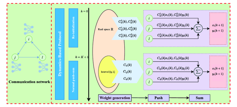
Based on the discussion of Algorithm 1, one can know that adopting the same weight for both and cause privacy (i.e., initial values) leakage. To solve the issue, a dynamics-based weight generation mechanism is developed in [33], whose details are outlined in Protocol 1.
The main idea of the dynamics-based mechanism is to confuse the state variables of the agents by injecting randomness into the mixing matrix in the initial few iterations. Fig. 1 briefly depicts the basic process. Obviously, the dynamics-based protocol has two stages. The first stage is from iteration to , which can be regarded as a re-initialization operation on the initial value. This stage is key to privacy protection. The second stage is from to , which can be viewed as the normal executions of the conventional push-sum method. This stage is key to ensuring convergence.
The dynamics-based method has been proved to reach an exact consensus point, and the sensitive information of legitimate agents is not inferred by honest-but-curious attackers in [33]. However, there are three significant challenges that have not been addressed: I) In the initial iterations, although each weight is arbitrary, the sum-one condition still imposes a constraint on the weight setting; II) The method cannot protect sensitive information from external eavesdropping attackers; II) Only asymptotic convergence of algorithms is discussed in most of the average consensus literature [30, 31, 32, 33, 34, 35], and analysis of the speed of convergence is rare.
To solve the above issues, we carefully redesign the push-sum rule to address I) and II), and III) is tackled in Section IV. From Protocol 1, one knows that the dynamics-based method mainly operates on the first iterations to preserve the privacy information. Specifically, the update rule of the -variable is given as
where is generated from Protocol 1. Note that the sum-one condition is used to ensure that the sum of all variables at each iteration is invariant, that is,
| (6) |
Thus, if we wish to circumvent the sum-one constraint, the new update rule must make (6) hold. Specifically, we take advantage of the fact that the amount of messages sent and received is equal for the entire system (i.e., the total mass of the system is fixed) and modify the update of the -variable as
| (7) |
with
where can take any value in (the sum-one condition is not required). One verifies that . Obviously, summing in (7) over yields (6). However, the update rule (7) is valid for honest-but-curious attacks and still ineffective for eavesdropping attacks, see Corollary 2. Thus, we further introduce an auxiliary parameter for , which is public information known for all agents, but not to the external eavesdropper. Details of our method are summarized in Algorithm 2.
| (8) | ||||
| (9) |
Remark 2.
Note that we mainly embed randomness for in the first iterations and do not consider . Since embedding randomness for alone can guarantee that for , and the auxiliary variable does not contain privacy information, so there is no need to embed randomness for either. Of course, if embedding randomness for is necessary, the update of the -variable in (9) is formulated as:
where and are generated in a similar way as and of Algorithm 2.
4 Convergence Analysis
Following Algorithm 2, it holds from the dynamics (8)-(9) that
| (10) | ||||
| (11) |
where and . It is clear from the settings of Algorithm 2 that: i) and are time-varying and column-stochastic; and ii) for .
Define and for . Particularly, and . Recursively computing (10) and (11), we can obtain
| (12) | ||||
| (13) |
where it holds for . Then, it follows that
| (14) | ||||
| (15) |
where we use the column stochasticities of and . For the first dynamics of in (8), using the fact that gives
| (16) |
which matches the relation (6). Combining (14) and (16) gives
| (17) |
Note that the dynamics of Algorithm 2 for iterations are analogous to the conventional push-sum method. Considering (17) in depth, it can be seen that the injected randomness of the first dynamics has no impact on the consensus performance. Next we show that Algorithm 2 can guarantee a linear convergence rate. Let .
Theorem 1.
Let be the sequence generated by Algorithm 2, and the network satisfies Assumption 1. Then, it holds, for all ,
where , and is a constant given as
where , and .
Proof.
Details of the analysis are outlined in Appendix A. ∎
Remark 3.
Theorem 1 indicates that Algorithm 1 can achieve an convergence rate with . Evidently, a smaller yields a better convergence rate. A straightforward way to obtain a smaller is to increase . However, it is essential to be aware that cannot be close to arbitrarily due to the nonnegativity and column stochasticity of the mixing matrix for . To satisfy the weight generation mechanism in Algorithm 2, it holds .
5 Privacy Analysis
We analyze that Algorithm 2 is resistant to both honest-but-curious and eavesdropping attacks.
5.1 Performance Against Honest-but-curious Attacks
For the honest-but-curious attacks, we make the following standard assumption.
Assumption 2.
Consider a strongly connected network , where some colluding honest-but-curious nodes exist. We assume that each agent has at least one legitimate neighbor, i.e., .
Remark 4.
Theorem 2.
Under Assumptions 1-2, the initial value of legitimate agent can be safely protected if during the running of Algorithm 2.
Proof.
Recalling the definition of privacy metric in Section II-D, it can be shown that the privacy of agent can be safely protected insofar as . The available information to is , where denotes the information available to each individual given as
with
To prove , it suffices to show that agents in fail to judge whether the initial value of agent is or where is an arbitrary value in and . Note that agents in are only able to infer using . In other words, if the initial value makes the information accessed by agents of unchanged, i.e., , then . Hence, we only need to prove that there is under two different initial values and .
Since , there exists at least one agent . Thus, some settings on initial values of agent and mixing weights associated with agent that satisfy the requirements in Algorithm 2 such that holds for any variant . More specifically, the initial settings are given as
| (18) |
where is nonzero and does not equal either or . Apparently, such an initial value setting has no impact on the sum of the original initial values. Then, we properly choose the mixing weights such that . Here, “properly” means the choosing mixing weights should obey the weight generation mechanism in Algorithm 2. Our analysis will be continued in two cases, and , respectively.
Case I: We consider . One derives if the weights are set as
| (19a) | ||||
| (19b) | ||||
| (19c) | ||||
| (19d) | ||||
| (19e) | ||||
| (19f) | ||||
| (19g) |
Case II: We consider . One derives if the weights are set as
| (20a) | ||||
| (20b) | ||||
| (20c) | ||||
| (20d) | ||||
| (20e) | ||||
| (20f) | ||||
| (20g) |
Combining Cases I and II, it can be derived that under the initial value . Then
Therefore, the initial value of agent is preserved against agents if agent has at least one legitimate neighbor . ∎
Remark 5.
By (19e) and (20e), one knows that the privacy of Algorithm 2 does not have any requirement for the weights and . The reason for this is that each agent in Algorithm 2 does not use such weights in the iterations . One benefit of this operation is that it allows the mixing weights of the transmitted information to be used in the iterations without requiring the satisfaction of the sum-one condition, which in turn provides better flexibility in the setting of mixing weights.
Corollary 1.
During the running of Algorithm 2, the initial value of agent would be revealed if holds.
Proof.
Recursively computing the update of -variable for yields
| (21) |
Then, using the column stochasticities of for and for , we have
Combining the above relations with (8) and (9), one arrives
| (22) | ||||
| (23) |
Further, combining the results in (21) and (22) gives
| (24) |
Note that each agent has access to . If holds for legitimate agent , all the information involved on the right sides of (23) and (24) is accessible to the honest-but-curious agents. Then, using and (23), agent can capture for all . Further, as for , can be inferred correctly by agent using
Making use of (24), the desired initial value is revealed. ∎
5.2 Performance Against Eavesdropping Attacks
For the eavesdropping attacks, we make the following assumption.
Assumption 3.
Consider a strongly connected network , where an external eavesdropper exists. We assume that the parameter is not accessible to the eavesdropper.
Theorem 3.
Proof.
From the definition of privacy metric in Section II-D, it is shown that all agents’ privacy can be safely protected insofar as . The available information to the external eavesdropper is given as
The dynamic (8) can be reformulated as
| (25) |
where denotes the incidence matrix associated network , and is a stack vector whose -th element is with being the -th edge in . Note that the external eavesdropper is only able to infer all using . To prove , it is required to indicate that any initial value makes the information accessed by the external eavesdropper unchanged, i.e., , where is any value in . Hence, we only need to prove that it holds under two different initial states and . Specifically, one derives if the weights are set as
| (26a) | ||||
| (26b) | ||||
| (26c) | ||||
| (26d) | ||||
| (26e) | ||||
| (26f) |
Further, owing to the fact that the rank of is and the nullity of is , one concludes that is any vector in . In other words, the probability of landing in the null space of is zero. Thus, for any , it holds
Naturally, can be any value in . Therefore,
That is to say, all initial values are preserved against the external eavesdropper. ∎
Corollary 2.
If the update rule for in (8) is substituted with (7), Algorithm 2 cannot preserve the initial value of each agent against eavesdropping attacks.
Proof.
Recursively computing the update of -variable in (7) for gives
| (27) |
Note that (22) and (23) still hold in this setting. Combining (27) with (22), we have
| (28) |
Since the external eavesdropper can capture all transmitted information, all terms in the right sides of (23) and (28) can be accessed by the external eavesdropper. Then, using and (23), agent can capture for all . Further, since for , can be inferred correctly by agent using
Making use of (28), the desired initial value is inferred. ∎
Remark 6.
According to the discussions above, it is evident that the first -step perturbations are crucial for preserving privacy against honest-but-curious attacks, while the time-varying parameter is pivotal in protecting privacy from eavesdropping attacks. Note that we only require that is agnostic to the eavesdropper. Although this requirement is extremely stringent in practice, it still has some developmental significance. Specifically, due to the arbitrariness of , we can mask only by some privacy-preserving techniques such as encryption and obfuscation. Since these techniques act only on , they do not impact the convergence of the algorithm.
Remark 7.
Theorem 1 states that the randomness of embeddings in the first iterations has no impact on the consensus performance. Besides, from the privacy analysis, we can see that only changing the mixing weights and auxiliary parameter at the iteration is enough to mask the initial values. That is, we can make Algorithm 2 protect the initial value by simply embedding randomness to (i.e., setting ). Here, our consideration of is to preserve more intermediate states , but this also delays the consensus process, see Fig. 3. Therefore, if the intermediate states are not information of privacy concern, we directly set to obtain the best convergence performance.
Discussion: The update rules of Algorithm 2 can also be extended to the case of vector states. Actually, privacy (i.e., the agent’s initial vector state) is naturally protected provided that each element of the vector state is assigned an independent mixing weights. The details are summarized in Algorithm 3.
| (29) | ||||
| (30) |
| Parameter | Iteration | Iteration |
|---|---|---|
| , where each , , is chosen from independently | ||
| Each is chosen from for with satisfying | ||
| , where each , , is chosen from for independently | , where is equal to | |
Corollary 3.
The following statements hold:
-
i)
Let be the sequence generated by Algorithm 3. Define as the average initial state. Under Assumption 1, it holds for all , where .
-
ii)
Let denote the set of honest-but-curious agents. Under Assumptions 1-2, the initial value of agent can be preserved against during the running of Algorithm 3;
-
iii)
Under Assumptions 1 and 3, the initial values of all agents can be preserved against eavesdropping attacks during the running of Algorithm 3.
Proof.
The proof of i) follows a similar path to Theorem 1, the difference lies only in the use of the Kronecker product and thus omitted. Then, by the setup of Table I, it is possible to make each element of the vector state hold an independent coupling weight. According to the analysis of Theorems 2-3, we can know that each scalar-state element in the vector state can be preserved against both honest-but-curious and eavesdropping attacks. Therefore, each vector state can also be preserved. ∎
6 Experiments Validation
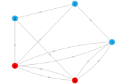
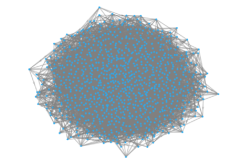
We construct simulations to confirm the consensus and the privacy performances of our methods. Two directed networks are built in Fig. 2.
6.1 Consensus Performance
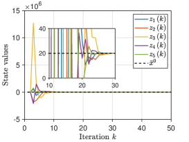
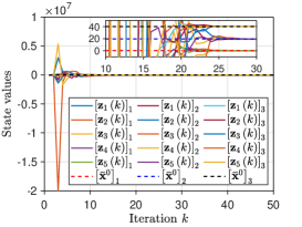
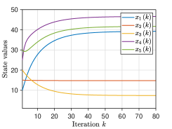
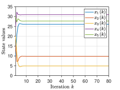
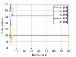
We pick the network and set . For Algorithm 2, at iteration , the mixing weights for are selected from . The initial states take values of , respectively, and thus . The parameter is generated from for all . For Algorithm 3, at iteration , the parameters are generated from for with , and the mixing weights are chosen from for and . Each component of the initial values , , is generated from the Gaussian distributions with different mean values . Fig. 3 plots the evolutionary trajectories of the state variables under , and shows the evolutions of over . One observes that: i) Each estimate converges to the average value , and a linear consensus rate is achieved; and ii) a larger means a worse consensus accuracy.
6.2 Comparison with other works
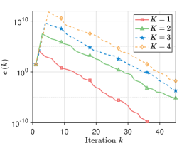
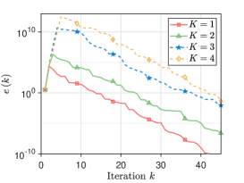
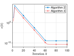
We compare our algorithms with three data-obfuscation based methods, i.e., the differential privacy algorithm [17], the decaying noise algorithm [21], and the finite-noise-sequence algorithm [22]. Here, we set , and the adopted mixing matrix is generated using the rules in [17]. Specifically, the element is set to if ; otherwise, . Since the directed and unbalanced networks are more generalizable than the undirected and balanced ones adopted in [17, 21, 22], these algorithms cannot achieve average consensus, as reported in Fig 4.
6.3 Effect of network degrees and Scalability
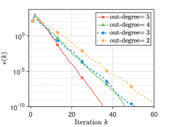
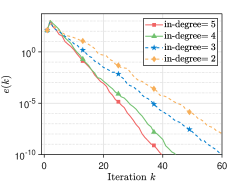
Since the proposed algorithms are performed on unbalanced directed networks, we use different networks to explore the effect of different degrees on the consensus rate. We simulate communication networks with agents. Specifically, a directed ring network connecting all agents is built. Then, in the first networks, each agent arbitrarily selects out-neighbors in order; in the last networks, each agent arbitrarily select in-neighbors in order. In this experiment, the variable are taken sequentially from the interval at intervals of . We set and . For the iterations , the mixing weights for are selected from , and the parameter is generated from . Moreover, we employ the network to demonstrate the scalability of the proposed algorithms. Each initial value or is generated from i.i.d . The parameters , , and take values of , , and , respectively. The mixing weights and the parameter or are generated in the same way as Section VI-A. As shown in Fig. 5, it is stated that i) As the out-degree or in-degree increases, Algorithm 2 has a faster consensus rate. A possible reason for this is that the increase in out-degree or in-degree leads to more frequent communication between agents, and thus more information is available for state updates, which in turn leads to a faster consensus rate; ii) The proposed algorithms still ensure that all agents linearly converge to the correct average value even if a large-scale network is used.
6.4 Privacy Performance
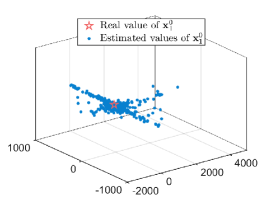
We evaluate the privacy-preserving performances of Algorithms 2 and 3. Under the network , we consider the initial value of the legitimate agent will suffer from the joint inference of honest-but-curious agents , and agent is legitimate. In the scalar-state case, we set and are generated from the Gaussian distributions with variance and zero mean, while the initial value and are randomly generated from i.i.d. in the vector-state case. Moreover, we set and the maximal iteration .
To infer , agents construct some linear equations based on their available information outlined below:
| (31a) | ||||
| (31b) | ||||
| (31c) |
where
Furthermore, agents can also construct, for ,
| (31d) |
where can be derived from
since for .
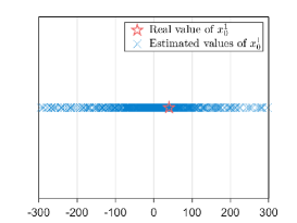
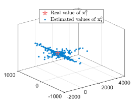
The number of linear equations is while that of unknown variables to is , including , , , , , , , and . Consequently, there are infinitely many solutions due to the fact that the number of equations is less than that of unknown variables. The analysis of the vector-state case is similar to that of the scalar-state case, so it will not be elaborated here. To uniquely determine , we use the least-squares solution to infer . In this experiment, agents in estimate or for times. Figs. 6a-6b show the estimated results. One can observe that agents in fail to obtain a desired estimate of or .
Next, we consider the case of eavesdropping attacks. The parameter settings follow the above experiment. To infer the value , the external eavesdropper constructs some linear equations below based on its available information :
| (32a) | ||||
| (32b) | ||||
| (32c) |
where
Further, the external eavesdropper can deduce from (32) that
| (33a) | ||||
| (33b) | ||||
| (33c) |
Obviously, all terms in the right side of (33) can be accessed by the external eavesdropper. Consequently, using , the eavesdropper can be aware of all , . Moreover, the external eavesdropper can capture and for . Then, for can be derived using
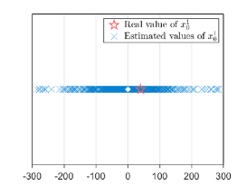
This implies that all information in (32b) and (32c) is captured by the external eavesdropper, which is considerably different from the case of honest-but-curious attacks. So, only (32a) has some unknown variables , and for the external eavesdropper. The vector-state case leads to the same results as the scalar-state case by following the same analysis path, so it is not stated again. In this experiment, we still use the least-squares solution to estimate . The external eavesdropper estimates or for times. Figs. 6c-6d show the estimated results. One observes that the external eavesdropper cannot obtain an expected estimate of or .
7 Conclusion
We proposed a dynamics-based privacy-preserving push-sum algorithm over unbalanced digraphs. We theoretically analyzed its linear convergence rate and proved it can guarantee the privacy of agents against both honest-but-curious and eavesdropping attacks. Finally, numerical experiments further confirmed the soundness of our work. Future research will consider efforts to prevent eavesdropping attacks under a weaker assumption, as well as consider efforts to protect privacy even after is removed.
CRediT authorship contribution statement
Huqiang Cheng: Methodology, Formal analysis, Writing - original draft. Mengying Xie: Methodology, Writing - review & editing. Xiaowei Yang: Supervision, Writing - review & editing. Qingguo Lü: Formal analysis, Writing - review & editing. Huaqing Li: Writing - review & editing, Funding acquisition.
Declaration of competing interest
The authors declare that they have no known competing financial interests or personal relationships that could have appeared to influence the work reported in this paper.
Data available
Data will be made available on request.
Acknowledgment
This work is supported by the National Natural Science Foundation of China (62302068 and 61932006).
References
- [1] H.-K. Bae, H.-O. Kim, W.-Y. Shin, S.-W. Kim, “How to get consensus with neighbors?”: Rating standardization for accurate collaborative filtering, Knowl.-Based Syst. 234 (2021) 107549.
- [2] Y. Yang, W. Tan, T. Li, D. Ruan, Consensus clustering based on constrained self-organizing map and improved Cop-Kmeans ensemble in intelligent decision support systems, Knowl.-Based Syst. 32 (2012) 101–115.
- [3] Z. Zhang, Y. Gao, Z. Li, Consensus reaching for social network group decision making by considering leadership and bounded confidence, Knowl.-Based Syst. 204 (2020) 106240.
- [4] F. C. Souza, S. R. B. Dos Santos, A. M. de Oliveira, S. N. Givigi, Influence of network topology on UAVs formation control based on distributed consensus, in: Proceedings of the IEEE International Systems Conference, 2022, pp. 1–8.
- [5] P. Wu, H. Huang, H. Lu, Z. Liu, Stabilized distributed online mirror descent for multi-agent optimization, Knowl.-Based Syst. 304 (2024) 112582.
- [6] D. Kempe, A. Dobra, and J. Gehrke, Gossip-based computation of aggregate information, in: Proceedings of 44th Annual IEEE Symposium on Foundations of Computer Science, 2003, pp. 482–491.
- [7] L. Xia, Q. Li, R. Song, Y. Feng, Dynamic asynchronous edge-based event-triggered consensus of multi-agent systems, Knowl.-Based Syst. 272 (2023) 110531.
- [8] F. Bénézit, V. Blondel, P. Thiran, J. Tsitsiklis, M. Vetterli, Weighted gossip: Distributed averaging using non-doubly stochastic matrices, in: Proceedings of 2010 IEEE International Symposium on Information Theory, 2010, pp. 1753–1757.
- [9] C. N. Hadjicostis, A. D. Domínguez-García, T. Charalambous, Distributed averaging and balancing in network systems: With applications to coordination and control, Found. Trends Syst. Control 5 (2–3) (2018) 99–292.
- [10] Z. Liu, Y. Li, G. Lan, Z. Chen, A novel data-driven model-free synchronization protocol for discrete-time multi-agent systems via TD3 based algorithm, Knowl.-Based Syst. 287 (2024) 111430.
- [11] W. Guo, H. Wang, W.-G. Zhang, Z. Gong, Y. Xu, R. Slowiński, Multi-dimensional multi-round minimum cost consensus models with iterative mechanisms involving reward and punishment measures, Knowl.-Based Syst. 293 (2024) 111710.
- [12] J. N. Tsitsiklis, Problems in decentralized decision making and computation, Ph.D. thesis, MIT, 1984.
- [13] Z. Zhang, M. Y. Chow, Incremental cost consensus algorithm in a smart grid environment, in: Proceedings of the IEEE Power and Energy Society General Meeting, 2011, pp. 1–6.
- [14] C. Dwork, F. McSherry, K. Nissim, A. Smith, Calibrating noise to sensitivity in private data analysis, in: Proceedings of the 3rd Theory Cryptography Conference, 2006, pp. 265–284.
- [15] Z. Huang, S. Mitra, N. Vaidya, Differentially private distributed optimization, in: International Conference on Distributed Computing and Networking, 2015, pp. 1–10.
- [16] E. Nozari, P. Tallapragada, J. Cortés, Differentially private average consensus: Obstructions, trade-offs, and optimal algorithm design, Automatica, 81 (2017) 221–231.
- [17] Z. Huang, S. Mitra, G. Dullerud, Differentially private iterative synchronous consensus, in Proceedings of the 2012 ACM Workshop on Privacy in the Electronic Society, 2012, pp. 81–90.
- [18] L. Gao, S. Deng, W. Ren, C. Hu, Differentially private consensus with quantized communication, IEEE Trans. Cybern. 51 (8) (2021) 4075–4088.
- [19] D. Ye, T. Zhu, W. Zhou, S. Y. Philip, Differentially private malicious agent avoidance in multiagent advising learning, IEEE Trans. Cybern. 50 (10) (2020) 4214–4227.
- [20] M. Kefayati, M. S. Talebi, B. H. Khalaj, H. R. Rabiee, Secure consensus averaging in sensor networks using random offsets, in: IEEE International Conference on Telecommunications and Malaysia International Conference on Communications, 2007, pp. 556–560.
- [21] Y. Mo, R. M. Murray, Privacy preserving average consensus, IEEE Trans. Autom. Control 62 (2) (2017) 753–765.
- [22] N. E. Manitara, C. N. Hadjicostis, Privacy-preserving asymptotic average consensus, in: European Control Conference (ECC), 2013, pp. 760–765.
- [23] S. Pequito, S. Kar, S. Sundaram, A. P. Aguiar, Design of communication networks for distributed computation with privacy guarantees, in: Proceedings of the 53rd IEEE Conference on Decision and Control, 2014, pp. 1370–1376.
- [24] I. D. Ridgley, R. A. Freeman, K. M. Lynch, Simple, private, and accurate distributed averaging, in: Proceedings of IEEE 57th Annual Allerton Conference on Communication, Control, and Computing, 2019, pp. 446–452.
- [25] A. Alaeddini, K. Morgansen, M. Mesbahi, Adaptive communication networks with privacy guarantees, in: Proceedings of American Control Conference, 2017, pp. 4460–4465.
- [26] M. Kishida, Encrypted average consensus with quantized control law, in: Proceedings of IEEE Conference on Decision and Control, 2018, pp. 5850–5856.
- [27] C. N. Hadjicostis, A. D. Dominguez-Garcia, Privacy-preserving distributed averaging via homomorphically encrypted ratio consensus, IEEE Trans. Autom. Control, 65 (9) (2020) 3887–3894.
- [28] W. Fang, M. Zamani, Z. Chen, Secure and privacy preserving consensus for second-order systems based on paillier encryption, Systems & Control Letters, 148 (2021) 104869.
- [29] M. Ruan, H. Gao, Y. Wang, Secure and privacy-preserving consensus, IEEE Trans. Autom. Control 64 (10) (2019) 4035–4049.
- [30] Y. Wang, Privacy-preserving average consensus via state decomposition, IEEE Trans. Autom. Control, 64 (11) (2019) 4711–4716.
- [31] X. Chen, L. Huang, K. Ding, S. Dey, L. Shi, Privacy-preserving push-sum average consensus via state decomposition, IEEE Trans. Autom. Control 68 (12) (2023) 7974–7981.
- [32] H. Cheng, X. Liao, H. Li, Q. Lü, Dynamic-based privacy preservation for distributed economic dispatch of microgrids, IEEE Trans. Control Netw. Syst. (2024) http://dx.doi.org/10.1109/TCNS.2024.3431730.
- [33] H. Gao, C. Zhang, M. Ahmad, Y. Wang, Privacy-preserving average consensus on directed graphs using push-sum, in: IEEE Conference on Communications and Network Security (CNS), 2018, pp. 1–9.
- [34] H. Gao, Y. Wang, Algorithm-level confidentiality for average consensus on time-varying directed graphs, IEEE Trans. Netw. Sci. Eng. 9 (2) (2022) 918–931.
- [35] Y. Liu, H. Gao, J. Du, Y. Zhi, Dynamics based privacy preservation for average consensus on directed graphs, in: Proceedings of the 41st Chinese Control Conference, 2022, pp. 4955–4961.
- [36] Y. Wei, J. Xie, W. Gao, H. Li, L. Wang, A fully decentralized distributed learning algorithm for latency communication networks, Knowl.-Based Syst. (2024) https://doi.org/10.1016/j.knosys.2024.112829.
- [37] S. Gade, N. H. Vaidya, Private optimization on networks, In: 2018 Annual American Control Conference (ACC), 2018, pp. 1402–1409.
- [38] H. Cheng, X. Liao, H. Li, Q. Lü, Y. Zhao, Privacy-preserving push-pull method for decentralized optimization via state decomposition, IEEE Trans. Signal Inf. Proc. Netw. 10 (2024) 513–526.
- [39] D. Han, K. Liu, H. Sandberg, S. Chai, Y. Xia, Privacy-preserving dual averaging with arbitrary initial conditions for distributed optimization, IEEE Trans. Autom. Control 67 (6) (2022) 3172–3179.
- [40] H. Gao, Y. Wang, A. Nedić, Dynamics based privacy preservation in decentralized optimization, Automatica, 151 (2023) 110878.
- [41] Y. Lin, K. Liu, D. Han, and Y. Xia, Statistical privacy-preserving online distributed nash equilibrium tracking in aggregative games, IEEE Trans. Autom. Control 69 (2024) 323–330.
- [42] H. Cheng, X. Liao, H. Li, Distributed online private learning of convex nondecomposable objectives, IEEE Trans. Netw. Sci. Eng. 11 (2) (2024) 1716–1728.
- [43] K. Liu, H. Kargupta, J. Ryan, Random projection-based multiplicative data perturbation for privacy preserving distributed data mining, IEEE Trans Knowl. Data Eng. 18 (1) (2005) 92–106.
- [44] S. Han, W. K. Ng, L. Wan, V. C. Lee, Privacy-preserving gradient-descent methods, IEEE Trans Knowl. Data Eng. 22 (6) (2009) 884–899.
- [45] N. Cao, C. Wang, M. Li, K. Ren, W. Lou, Privacy-preserving multi-keyword ranked search over encrypted cloud data, IEEE Trans. Parallel Distrib. Syst. 25 (1) (2013) 222–233.
- [46] E. Seneta, Non-negative matrices and markov chains, Springer, 1973.
- [47] J. A. Fill, Eigenvalue bounds on convergence to stationarity for nonreversible markov chains with an application to the exclusion process, Ann. Appl. Probab. 1 (1) (1991) 62–87.
- [48] R. A. Horn, C. R. Johnson, Matrix Analysis, Cambridge university press Press, 2012.
- [49] Y. Lu, M. Zhu, On privacy preserving data release of linear dynamic networks, Automatica 115 (2020) 108839.
- [50] A. Machanavajjhala, D. Kifer, J. Gehrke, M. Venkitasubramaniam, -diversity: Privacy beyond -anonymity, ACM Trans. Knowl. Discovery Data 1 (1) (2007) 3–es.
- [51] A. Nedić, A. Ozdaglar, P. A. Parrilo, Constrained consensus and optimization in multi-agent networks, IEEE Trans. Autom. Control 55 (4) (2010) 922–938.
- [52] P. Paillier, Public-key cryptosystems based on composite degree residuosity classes, in: International conference on the theory and applications of cryptographic techniques, 1999, pp. 223–238.
Appendix A Proof of Theorem 1
Proof.
We divide the convergence analysis into two cases.
Case I: We consider the case of . It holds . Recalling (12) and (13), we have, for ,
| (34) | ||||
| (35) |
Referring [51, Corollary 2], there exists a sequence of stochastic vectors such that, for any ,
where and . Moreover, . Thus, it follows that, for ,
| (36) |
where . Since , it holds that for . So (34) and (35) can be evolved as
| (37) | ||||
| (38) |
It follows from [51, Corollary 2] that for any . Using the relation (16), one arrives
| (39) |
Combining (37) and (38) with (39) yields
where
Then, we can bound as
where the second inequality uses the relation , and the last inequality is based on and . Further taking into account (36), one derives that
Thus, we arrive that
| (40) |
where . Consequently, for , we have .
Case II: We consider the case of . Using , one has
Then, we compute as
where the last inequality uses the relation for all and . Specifically, as is a stochastic vector, holds, which in turn gives . Thus, it yields that
where and .
Combining Cases I and II and defining
| (41) |
one derives, for all ,
which is the desired result. ∎