Dynamics of fluctuations in an optical analogue of the Laval nozzle
Abstract
Using the analogy between the description of coherent light propagation in a medium with Kerr nonlinearity by means of nonlinear Schrödinger equation and that of a dissipationless liquid, we propose an optical analogue of the Laval nozzle. The optical Laval nozzle will allow one to form a transonic flow, in which one can observe and study very unusual dynamics of classical and quantum fluctuations, including an analogue of the Hawking radiation of real black holes. Theoretical analysis of these dynamics is supported by numerical calculations, and estimates for a possible experimental realization are presented.
pacs:
42.65.Sf; 47.40.HgBlack hole radiation is one of the most impressive phenomena at the intersection of general relativity and quantum field theory. Accounting for the quantum nature of the physical vacuum led to the prediction that a black hole, defined classically as an object that even light cannot escape, in fact can be characterized by a temperature, entropyBekenstein and moreover emits thermal radiationH75 . Since direct experimentation with black holes is hardly possible, it was suggested to consider analogous phenomena in condensed matter physics where the ”high-energy” (short-wavelength) physics is known U81 . The suggestion was based on the observation that the derivation of the Hawking radiation uses only the linear wave equation in curved space-time, and not the Einstein equations. The same conditions for wave propagation arise when considering sound propagation in a fluid when the background flow is non-trivial U81 . This similarity was shown to be sufficient for applying the original considerations by Hawking, predicting the existence of thermal radiation of quantum origin from the fluid counterpart of the horizon, which can be called Mach horizon (where the fluid velocity equals the sound velocity, i.e. Mach number ). These ideas were further developed for possible applications in BEC fluids and other systems R00 ; BLV03 ; CFRBF08 ; RPC09 ; NBRB09 . As for experimental realizations, a white hole horizon was observed in optical fibersPKRHKL08 , where the probe light was back-reflected from a moving soliton, and a black hole horizon was observed in a BEC systemLIBGS09 .
We propose an experimental setup capable of creating a Mach horizon in an optical medium with Kerr nonlinearity, which may be called optical Laval nozzle. The propagation of weakly nonlinear coherent optical pulses is described by the non-linear Schrödinger (NLS) equation
| (1) |
It assumes the paraxial approximation, according to which the electric field of the light wave is written as , where is weakly dependent complex amplitude of the light propagating in the direction. The time coordinate is converted into the coordinateA95 which describes the shape of the light pulse in the moving coordinate system. The radius vector differential is now (anomalous dispersion) or (normal dispersion). is the equivalent external potential created by spacial variation of the refraction index in the medium and does not depend on .
Now we briefly sketch the fundamental resultU81 as applied to coherent light propagation in a medium with Kerr nonlinearity. The Madelung transformationM27 (see alsoM75 ; DFSS07 ; Marino08 ) maps the NLS eq.(1) on two equations
| (2) | |||
| (3) |
for an equivalent fluid with density and velocity . For permanently shined light the coordinate is redundant. is a ”quantum potential” corresponding to . The light wave vector is the ”particle mass” and the velocity is dimensionless.
Linearizing Eqs. (2) and (3) with respect to the small fluctuations and around a steady solution and , we arrive at
| (4) |
where the metric with the determinant is given by the interval
| (5) |
with . The ordinary ”sound waves” in the effective fluid arise as solutions of eq. (4) around the equilibrium solution , and , that exists at , so that is the squared sound velocity. The nonlinearity coefficient is positive, , otherwise the ”sound velocity” becomes imaginary and various instabilities, such as collapsing solitonsS90 arise. Eq. (4) may include corrections due to the quantum potential, which may be of importance for short waves.
The background flow may arise in the Laval nozzleS65 ; LL87 , i.e. a vessel with variable cross-section , whose application to some condensed-matter analogues was discussed inSakagamiOhashi ; BLV03a . The flow velocity increases with decreasing , and reaches the sound velocity in the narrowest part of the vessel, called the throat. Further acceleration is reached by increasing . Here we analyze the transonic flow for the optical realization of the Laval nozzle shown in Fig. LABEL:Laval.
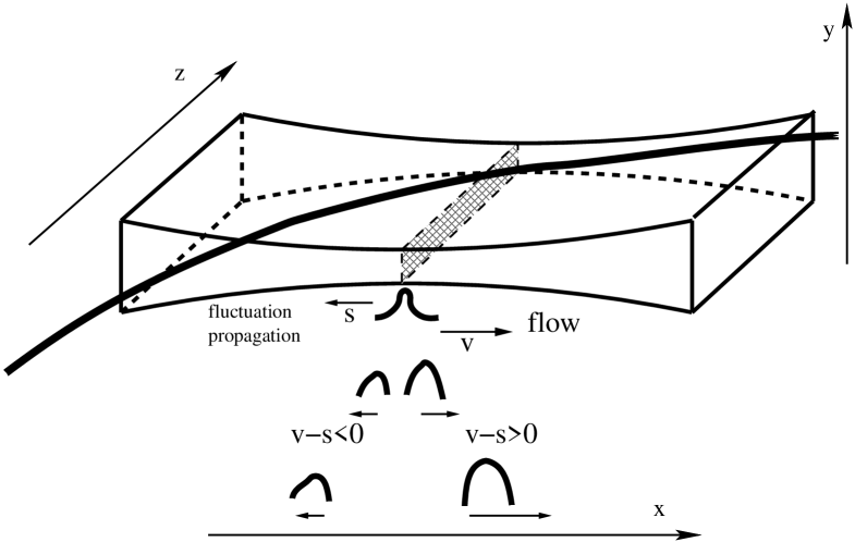
The laser beam, nearly parallel to the axis, is tilted in the direction by an angle , i.e. the initial phase in the electric field amplitude is . plays the part of ”flow velocity” in the direction. Acceleration of the flow within the plate of variable width ( - axis) results in bending of the beam ( increases) as shown in Fig. LABEL:Laval. It leads to small corrections to , quadratic in . We always assume that the wave length is smaller than all the other relevant scales.
Now we consider the flow bounded by the walls of a hyperbolic shape
| (6) |
with sliding boundary conditions, and the elliptic coordinates are introduced, with . From the symmetry considerations the flow is along the x axis for , i.e. .
Equation (2) for a steady flow becomes
where and and are the velocity components in the elliptic coordinates.
This equation is satisfied if
| (7) |
where and are functions only of and respectively, and is a constant. Since the transversal velocity is zero at the throat at we get that .
We assume the streamlines in the vicinity of the central line, i.e. small , to be close to the lines of constant . Then calculating the covariant derivatives in the curvilinear elliptic coordinates and neglecting in the result the second order corrections in , Eq. (3) reads (cf., LL87 )
| (8) |
The flow reaches the sound velocity at . The second Eq. (7) in the elliptic coordinates results in with , and finally, using Eq. (8), we get , where overlined quantities refer to the throat. The coordinate dependence of the density immediately yields the coordinate dependence of the sound velocity . Correspondingly the values of these quantities at the throat are connected as .
We may now represent Eq. (4) in the narrow transonic region in the dimensionless form
| (9) |
where . The coefficients , and are obtained above for the hyperbolic Laval nozzle. However, the ratio holds for any differentiable shape of this type. We look for a solution of Eq. (LABEL:b9) in the form , where the functions are linear combinations of the two sets of eigen functions
| (10) |
In a background flow characterized by a space independent velocity, eq. (9) has the form of a one-dimensional Klein-Gordon wave equation for the field in a flat space. Then one obtains two plane waves propagating to the left (against the flow) and to the right (with the flow). In the considered here transonic case, when the background flow velocity and speed of sound vary with the coordinate, the left moving plane wave transforms into the eigen mode , which is a function with a branching point near , whereas the right moving plane wave is characterized by the nonlinear spectral relation
| (11) |
The complex wave vector for the real ”frequencies” reflects the fact that the coordinate of these eigen modes corresponds to motion along diverging hyperbolic streamlines. However, the frequency is real which indicates linear stability of the flow with respect to weak fluctuations.
The corresponding eigen modes
| (12) |
for the density fluctuations can be obtained directly from the linearization of the Euler equation (3).
Crossing the Mach horizon at , the solution acquires the factor . The same factor appears when considering quantum fluctuations. Following the logic of H75 (also discussed in detail in DL08 — eqs. (2.88)-(2.90)) this results in radiation to the left of the Mach horizon (outside the ”black hole”) with the frequency distribution . This distribution has the same form as a Planck distribution for black body radiation, with the parameter in physical dimensions. The latter plays a role similar to that of the Hawking temperature in black hole radiation. However the quantity is not a real physical temperature. The part of time is played here by the spatial coordinate , i.e. the ”frequency” is the wave vector of a fluctuation in the direction. This ”temperature” is measured in units of momentum rather than energy, and the corresponding ”thermal fluctuations” are waves along the direction with a typical wavelength of order .
A ”straddled” fluctuation
| (13) |
( is the step function) with a Gaussian spectral density around a positive frequency of a width is composed exclusively of the ”left moving” normal modes , singular at . Its ”time” evolution (i.e. dependence) is determined by the envelope function The ”frequencies” of these oscillations on both sides of the horizon strongly vary with . This is reminiscent of ”time slowing” near the horizon of a real black hole.
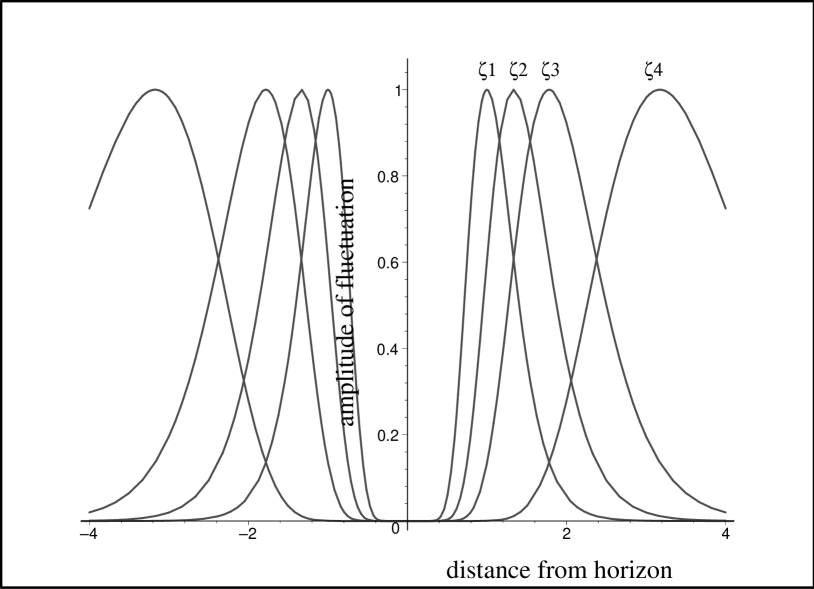
Fig. 2 shows how the maxima of the fluctuation amplitude propagate on both sides of the Mach horizon, with zero amplitude on the horizon. The part residing to the right side of the horizon (the supersonic region, ) should be multiplied by the factor (not shown in Fig. 2), with the Hawking temperature as a parameter. Therefore the ratio of amplitudes of a classical fluctuation on the left and the right of the horizon directly measures the Hawking temperature.
The fluctuation moves against the transonic flow with the velocity of sound. Its left part escapes to the left against the subsonic background flow, and moves with a very small velocity to the left. The right part of the fluctuation is ”flushed” away by the supersonic flow (see Fig. LABEL:Laval), and moves to the right with a small velocity . Here and are the subsonic flow velocity and local speed of sound of the flow in the vicinity and to the left of the Mach horizon, whereas and are the corresponding quantities in the supersonic region to the right of the Mach horizon (Note that for the symmetrical potential and spectral content of the fluctuation studied here the propagation on the two sides of the horizon is approximately symmetrical, as shown in Fig. 2). Using the eigen modes (Dynamics of fluctuations in an optical analogue of the Laval nozzle) for the density fluctuations we get a similar picture. In the case of quantum fluctuations the part moving to the left is analogous to the Hawking radiation observable outside the black hole. The part moving to the right is not observable in a real black hole. However in our case the supersonic region is accessible for observation.
The normal modes in (10) are plane waves propagating to the right in the direction of the flow with the velocity This velocity is twice the sound velocity, i.e. the sound velocity on the background of the supersonic flow, for large enough ”frequencies” . At small frequencies the propagation velocity is closer to thrice the sound velocity, i.e. twice the sound velocity relative to the background flow. If we use the analogy with the real black holes this result would correspond to superluminal motion. However there is no paradox here since the wavelength is larger than the throat width in the Laval nozzle, (in physical units). Hence we deal with the narrow field effect, analogous to superluminal propagation in near field optics and tunneling BK01 ; MRR00 ; MRS98 , which does not violate causality.
The above results are illustrated by numerical simulations of the NLS eq. (1) in 1 + 2 dimensions using a finite-difference approach based on the split-step Crank-Nicholson method.MA09 The potential is zero outside the hyperbola (6) and a negative constant inside. A packet with a Gaussian density distribution is given a Galilean boost in the fashion similar to Ref.FPR92 with a velocity close to that of sound for the density in the maximum of the Gaussian. This configuration differs from the discussed in the analytical part of the paper and is chosen for its relative simplicity and due to the fact its experimental realization seems to be rather straightforward. Although it differs in many aspect such as strongly nonhomogeneous distribution of the density and, hence, of the sound velocity, which is also affected be the quantum potential contribution, this configuration may be very convenient and useful for studying propagation and classical fluctuations in the optical Laval nozzle.
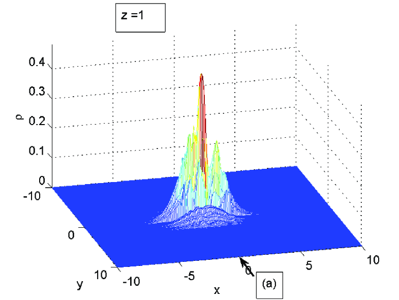
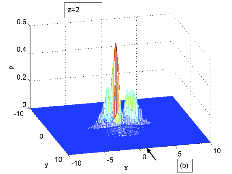
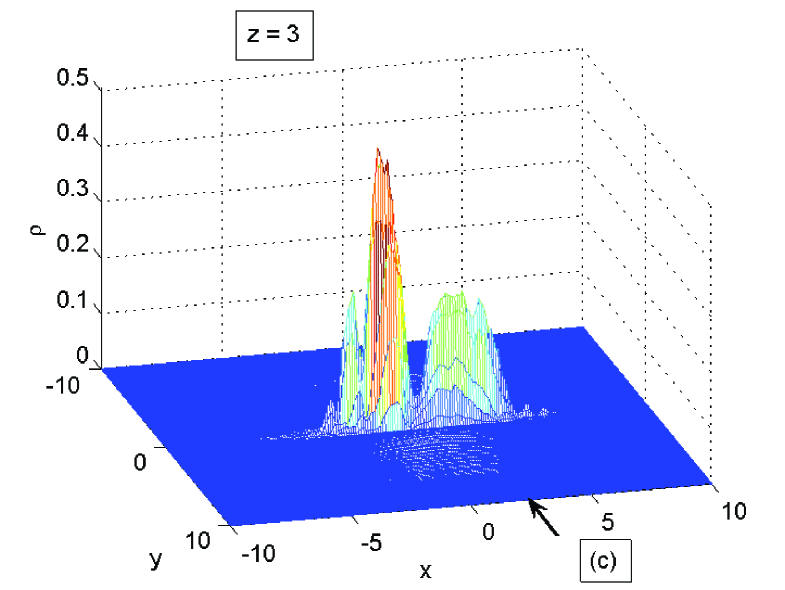
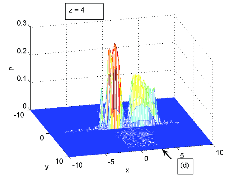
The calculation is carried out for Eq. (1) with and , whereas the amplitude function is normalized to unity. The depth of the potential in the nozzle . It has a hyperbolic shape with and . Meaning that its half-width is 0.3 at the throat at and 0.5 at . The Gaussian centered initially at is given a boost with the phase corresponding to the unit velocity. Figs. 3 show the packet at four successive stages of its propagation. A straddled fluctuation gradually develops with a characteristic dip close to the throat of the nozzle, which becomes deeper and nearly cuts the original packet in two. The fluctuation in this case becomes strong and in the end consumes a major part of the packet.
Since the numerical code deals with the NLS eq. (1), it solves a nonlinear problem strongly deviating from the steady transonic flow assumed in the above analysis, and fully accounts for the quantum potential. The density is strongly nonhomogeneous which leads to a nonhomogeneous distribution of the sound velocity. The latter should be also corrected by the contribution of quantum potential which cannot be considered small anymore. The Gaussian packet evolves into a two hump structure permanently changing its shape with the propagation length (”time”), as is clearly demonstrated in Figs. 3.
There are such factors as quantum potential (dispersion) and defocusing nonlinearity, which may influence the dynamics of the packet and in principle also cause its splitting in two parts. Control calculations of the packet moving in free space, or in a potential well with parallel walls do not show the type of behavior shown in Fig. 3. Decreasing the boost velocity also weakens the effect. Otherwise the general pattern presented in these figures is rather robust and holds when varying the parameters as long as the packet is boosted in a hyperbolically shaped potential well.F
The above ideas can be tested experimentally by launching a continuous wave laser beam through an appropriately shaped nozzle, with reflective walls, filled with a Kerr-like defocusing nonlinear material. Such a one-dimensional nozzle can be constructed from two convex cylindrical mirrors, put back to back at an adjustable separation with the space between them sealed and filled with a nonlinear liquid such as iodine-doped ethanolJason . The nonlinear coefficient of the solution can be expressed, in terms of the nonlinearly-induced refractive index change , as , where is the linear refractive index of the materialJason . The corresponding dimensionless sound velocity is . Assuming a nonlinear index change of 1%, an incoming laser beam would emulate supersonic flow when , i.e. when the input angle of the beam is larger than degrees. The required input angle for observing transonic acceleration through the nozzle is therefore technically feasible. The acceleration can be controlled by mechanically varying the throat width, and monitored by observing the deflection of the laser beam as it traverses the nozzle. The intensity and phase profile of the beam coming out of the experimental setup can be studied using standard detection and interferometric techniques. These would allow measurement of the transverse acceleration of the beam, as well as detection and characterization of classical fluctuations that propagate away from the throat region. such classical fluctuations may be introduced by locally perturbing the optical fluid in a deterministic fashion, e.g. by injecting a second narrow laser beam into the nozzle throatMarino08 .
Constructing a Laval nozzle of hyperbolic shape might not be easy, but we believe that most of the effects discussed above will also be observed in other types of convergent-divergent nozzles (in fact many aeronautical applications of the Laval nozzle are not hyperbolically shaped). Otherwise the proposed experimental setup is quite simple and straightforward to implement in a table-top experiment, in particular as compared to the previously proposed rotating black hole configurationMarino08 and to water tank experimentsRousseaux08 . The (classical) fluctuations will be observed directly, superimposed on an otherwise smooth transverse beam profile, and in principle will not require as high a dynamic range as previous optical experimentsPKRHKL08 . The experiment is also more straightforward than other proposed schemes, e.g. those based on SQUID array transmission lines NBRB09 and atomic BECCFRBF08 ; RPC09 .
In summary, we demonstrate the possibility of creating an optical analogue of the Laval nozzle. The interesting point will be to study the dynamics of straddled fluctuations which may be either quantum or classical and even artificially created. The equivalent of the Hawking temperature enters as an important parameter characterizing all types of fluctuations. This temperature is measured in units of momentum, rather than energy, which corresponds to a wavelength exceeding the width of nozzle throat by about two orders of magnitude, and in principle accessible for experimental measurements. Numerical simulations support the theoretical findings but also indicate that the phenomenon is much more complicated and interesting.
Acknowledgments. Support of Israeli Science Foundation, Grant N 944/05 and of United States - Israel Binational Science Foundation, Grant N 2006242 is acknowledged. VF is grateful to Max Planck Institute for Physics of Complex Systems, Dresden, for hospitality and to G. Shlyapnikov and N. Pavloff for stimulating discussions.
References
- (1) Bekenstein J. D., Phys. Rev. D 7, 2333 (1973).
- (2) Hawking S. W., Commun. Math. Phys. 43, 199 (1975).
- (3) Unruh W. G., Phys. Rev. Lett. 46, 1351 (1981).
- (4) Reznik B., Phys. Rev. D62, 044044 (2000).
- (5) Barcelo C., Liberati S., Visser M., Phys. Rev. A 68, 053613 (2003).
- (6) Carusotto I., Fagnocchi S., Recati A., Balbinot R. and Fabbri A., New Journal of Physics 10, 103001 (2008).
- (7) Recati A., Pavloff N., and Carusotto I., Phys. Rev. A 80, 043603 (2009).
- (8) Nation P. D., Blencowe M. P., Rimberg A. J., and Buks E., Phys. Rev. Lett. 103, 087004 (2009).
- (9) Philbin T. G., Kuklewicz C., Robertson S., Hill S., König F., Leonhardt U., Science, 319, 1367 (2008).
- (10) Lahav O., Itah A., Blumkin A., Gordon C., Steinhauer J., arXiv:0906.1337v1.
- (11) Agrawal G. P., Nonlinear Fiber Optics, Aacademic Press, New York (1995).
- (12) Madelung E., Z. Phys. 40, 322 (1927).
- (13) Marburger J. H., Prog. Quant. Electr., 4, 35 (1975).
- (14) Dekel G., Fleurov V., Soffer A. and Stucchio C., Phys. Rev. A 75, 043617 (2007).
- (15) Marino F., Phys. Rev. A 78, 063804 (2008).
- (16) Silberberg Y., Opt. Lett. 15, 1283 (1990).
- (17) Sedov L. I., Two Dimensional Problems in Hydrodynamics and Aerodynamics, Interscience Publ., New York, 1965.
- (18) Landau L. D. and Lifshits E. M., Fluid Mechanics, Pergamon Press, Oxford, 1987.
- (19) Sakagami M. and Ohashi A., Prog. Theor. Phys. 107 (6), 1267 (2002).
- (20) Barcelo C., Liberati S., and Visser M., Int. J. of Mod. Phys. A 18, 1 (2003).
- (21) Damour T. and Lilley M., arXiv:0802.4169v1 [hep-th] (2008).
- (22) Broe J. and Keller O., Journal of Microscopy, 202, 286 (2001).
- (23) Mugnai D., Ranfagni A. and Ruggeri R., Phys. Rev. Lett. 84, 4830 (2000).
- (24) Mugnai D., Ranfagni A. and Schulmann L.S., Phys. Lett. A247, 291 (1998).
- (25) Muruganandam P., Adhikari S.K., arXiv:0904.3131v [cond-mat.quant-gas] (2009).
- (26) Frisch T., Pomeau Y., and Rica S., Phys. Rev. Lett. 69, 1644 (1992).
- (27) Barsi C., Wan W., Sun C., and Fleischer J. W., Opt. Lett. 32, 2930 (2007).
- (28) Rousseaux G., Mathis C., Maïssa P., Philbin T. G., and Leonhardt U., New Journal of Physics 10, 053015 (2008).