Dynamics–Decoupling Control for Strings
of Heterogenous Nonlinear Autonomous Agents

Şerban Sabău^♯, Irinel–Constantin Morărescu^⋆, Lucian Buşoniu^‡
and Ali Jadbabaie^† ^♯Şerban Sabău is with the Electrical and Computer Engineering Dept., Stevens Institute of Technology, Hoboken, New Jersey, U.S.A. email: ssabau@stevens.edu^⋆ I.-C. Morărescu is with Université de Lorraine, CRAN, UMR 7039 and CNRS, CRAN, UMR 7039, 2 Avenue de la Forêt de Haye, 54506 Vandœuvre-lès-Nancy, France. email: constantin.morarescu@univ-lorraine.fr^‡ L. Buşoniu is with Technical University of Cluj–Napoca, Romania. email:lucian@busoniu.net^† Ali Jadbabaie is with the Institute for Data Systems and Society and the Laboratory for Information and Decision Systems, Massachusetts Institute of Technology. email: jadbabai@mit.edu.The work of I.C. Morărescu was partially funded by ANR project Computation Aware Control Systems (COMPACS) and the project NETASSIST funded by the Agence Universitaire de la Francophonie (AUF) and the Romanian Institute for Atomic Physics (IFA)

Abstract

We introduce a distributed control architecture for a class of heterogeneous, nonlinear dynamical agents moving in the “string” formation, while guaranteeing trajectory tracking, collision avoidance and the preservation of the formation’s topology. Each autonomous agent uses information and relative measurements only with respect to its predecessor in the string. The performance of the scheme is independent of the number of agents in the network and also on the agent’s relative position in the network. The scalability is a consequence of the “decoupling” of a certain bounded approximation of the closed–loop equations, which allows the regulation and controller design (at each agent) to be done individually, in a completely decentralized manner. A practical method for compensating communication induced delays is also presented. Numerical examples illustrate the effectiveness and the main features of the proposed approach.

I Introduction

Practical algorithms for distributed control of dynamically coupled systems are needed in many diverse applications raging from formation control of autonomous mobile agents [1, 2], synchronization of local clocks offsets or phase differences between (neighboring) coupled oscillators [3] or synchronous generators in power networks, sensor networks, load balancing [4], distributed agreement algorithms, cooperative control of multi-robot systems [5], opinion dynamics etc. In the specific setting of autonomous agents, the intricacies of dynamical coupling are not caused by the structure of the plant but rather by: (i) the structure of the cost functional resulting from the definition of the regulated measurements (e.g. in formation control - the inter-agent spacing distances defining the topology of the formation) and (ii) the coupling induced in the entailing feedback loop (with the distributed controller). The subsequent controller design problem is further complicated by the constraints to be imposed on the sensing and communications radii¹¹1By communications radius we mean the number of hops associated to an agent in the communications graph. The communications graph designates for each agent the neighbors with which it is able to communicate. of each agent.

The goal of the distributed control scheme is for all the agents to attain certain types of global collaborative behavior, such as their outputs/states reaching agreement in a precisely defined metric. In modern control parlance this class of objectives have been dubbed consensus [6, 7] and synchronization [8, 9, 10, 11, 12] problems. In the existing literature there is no clear demarcation line for this terminology (consensus versus synchronization), therefore we refer to [13, Section 1], [14, Section 1] for a useful discussion. It is worth mentioning that synchronization is a far more ambitious objective than classical reference tracking [15, Chapter 5.4], not only due to the distributed nature of the problem but also because the reference signals are never explicitly available to all agents, while in certain scenarios the synchronization trajectory is not even assigned beforehand and therefore there is no explicit reference to be tracked [14].

In this paper we deal with a group of heterogenous, nonlinear dynamical agents that solve a conventional agreement task (velocities matching in our case) but to which we append a specific set of constraints linking the individual states of two adjacent agents (in our case their positions in space). It turns out that the inclusion of such constraints render existing methods in distributed synchronization (e.g. distributed output regulation) inapplicable directly. The constraints relate to the inter-spacing distance between two agents, defined as the difference of their individual positions in space. In distance-based formation control²²2When referring to the position in space of an autonomous agent within a group of agents, the position must be defined with respect to an inertial system of reference common to all agents, e.g. a Global Positioning System. Note that the methods described here do not employ positioning systems, relying exclusively on measurements of relative distances between agents (acquired using for example onboard lidars). such constraints on the inter-spacing distances between neighboring agents arise naturally when: (i) defining the formation’s steady-state topology and (ii) when framing the collision avoidance requirement, via restrictions on inter-agent distances in the transitory regime. For illustrative simplicity we will only look at the string graph, while our method handles the heterogeneity of the formation and the inter-agent communications time delays, overlooking applications in the automotive industry. For consistency, we will refer to this setting as a synchronization problem.

Existing results in distributed synchronization (or distributed agreement) for Linear and Time Invariant (LTI) dynamics rely on observer-based distributed controllers [13, 16, 17], while the results from [18, 19, 20] remove the necessity of communicating the internal states of the local observers/sub-controllers and rely solely on the communication of the agents’ outputs. The results [21, 22, 23] for the heterogenous case, rely on the existence of a (virtual) exo-system generating the reference trajectory, while [24] outlines the intrinsic connections between the set of possible agreement trajectories and the sharing of all agents of certain “common dynamics”. The authors’ recent results in [25] provide a solution in the more ambitious setting of a distributed $\mathcal{H}_{2}/\mathcal{H}_{\infty}$ disturbances attenuation problem for the string graph, encompassing heterogenous agents and communications induced time delays. In this context, the current paper can be looked at as an extension to nonlinear control of the novel ideas for LTI dynamics from [25].

Theoretical advancements for nonlinear agents are in an incipient phase and have only been available more recently. The Lyapunov function approach in [26] is based on differential inequalities. The results in [27] pertaining to weakly minimum phase nonlinear agents are viable only under a passivity hypothesis, while those in [28, 29] pertain to globally Lipshitz-like conditions on the nonlinearities and leader-following networks. The reference [30] brings forward a necessary condition but no controller synthesis procedure while in [31] the agreement objective can only be set to a constant. Very recent results applicable to more complicated nonlinear dynamics include feedforward schemes [32] or are set up as cooperative output regulation problems e.g. [33, 34, 35, 36] and the references within, among which [33, 34] deal with leader-following networks. A notable feature of [35, 36] and especially [14] is that the sub-controller corresponding to an agent can be designed independently to all other sub-controllers. The downside of [35, 36] is the requirement of full state information exchange among agents, requirement entirely circumvented in [14] in a generic setting.

I-A Motivation and Scope of Work

The references above deal with the standard setup in which agents must achieve agreement of certain, pre-specified variables from each agent’s own state-space. For the class of problems treated in this paper, this takes the form of guaranteeing velocity matching in the steady-state, irrespective of the velocity profile of the leader (whose trajectory represents the reference for the entire formation) and which is seen as an adversarial player. However, the problem statement is further complicated by the inclusion of constraints that impose a substantial “coupling” between individual state variables of distinct agents, where these states represent the positions of agents³³3See also footnote 2 on page one.. These constraints cast on the relative distances between two neighboring agents render the existing methods referred above inapplicable directly⁴⁴4Existing results [37, 38, 39] on graph rigidity show how easy it is for these types of constraints to cause certain variations of this formulation of the distance-based formation control problem to become not well-posed. That happens when in an effort to preserve the topology of the formation, the controller encounters simultaneously conflicting constraints.. However, the constraints are needed in order to frame sufficient conditions for: (i) collision avoidance in the transitory regimes and (ii) topology preservation of the formation in steady-state (i.e. the interspacing distances between agents must converge asymptotically to certain pre-specified, constant values).

For high performance displacement-based formation control [40, Section 6], global positioning systems are not viable due to their relative large latencies and problematic reliability. The absence of a global coordinate system (combined with the fact that we avoid the use of accelerometers⁵⁵5Longitudinal accelerometers are notoriously unreliable for applications in the automotive industry.) requires that the agents must rely only on real time measurements of relative variables with respect to their neighbors, with all the difficulties such schemes entail, including the fact that collision avoidance and topology preservation cannot be reduced to a cooperative, output regulation problem (as those referred above).

I-B Contributions of the Paper

Our controller’s architecture is borrowed from platoon control literature⁶⁶6The conceptual architecture behind such distributed control schemes have been dubbed Cooperative Adaptive Cruise Control in the platooning control parlance [41, 25]. and is conceptually different from the aforementioned methods (e.g. [33, 34, 14] and the references within). Unlike [33, 34] it doesn’t require exchange of internal states (plant internal states or controller states) among agents. In turn, each agent needs to transmit its control action only to its immediate follower in the string. Furthermore, the design of each sub-controller, (“local” to an agent ) can be done in a completely independent manner - feature which is known to be especially challenging in distributed synchronization (see [14] and the references within for a comprehensive discussion in a related setting). Indeed, solely the knowledge of the dynamical model of the immediate predecessor is required for the local sub-controller at each agent, but once this is made available the regulation and controller design (at each agent) is done individually, in a completely decentralized manner.

Perhaps the most appealing feature of the proposed scheme is a particular dynamic “decoupling” of a certain bounded approximation of the closed–loop equations, entailing that individual, local analyses of the closed–loop stability at each agent will in turn guarantee the aggregated stability of the entire formation. This entails a complete scalability with respect to: (i) the number of agents in the string and (ii) the same performance irrespective of the relative position in formation (front or back of the string).

By comparison to our method, the main result in [42] is restricted to an undirected topology of the distributed controller, with stringent requirements involving: (i) the transmission of the exact state of the leader to many agents in the formation (virtual leaders) and (ii) the necessity of high control gains (see the last paragraph in [43, page 1] for a more detailed discussion).

Overall, our scheme improves on existing results in the following essential aspects:

1.

The agent dynamics are permitted to be heterogenous as long as they are nonlinear, globally Lipschitz.
2.

The agents achieve the synchronization of their velocities in the steady-state, while guaranteeing collision avoidance.
3.

The scheme guarantees steady-state topology preservation. Very recent results [44] are able to achieve this but only for identical single-integrators, exploiting an adaptation of the Cucker-Smale type nonlinear controllers [45]. Collision avoidance is obtained in [46] for single-integrators but without topology preservation.
4.

The distributed controller determines a “dynamic decoupling” of the closed loop, rendering the same performance independent of the number of agents or the relative position in formation. (The Lyapunov function guaranteeing the closed-loop stability of the entire formation is actually the sum of “local” Lyapunov functions, proper to each agent. This decoupling is also the root cause of the feature stated at the next point.)
5.

Completely independent regulation and controller design at each agent, under the sole requirement that each agent knows the dynamical model of its predecessor⁷⁷7This aspect is essential when dealing with merging/exiting of agents, since it allows only local reconfigurations (at the merging agent or at the follower of the exiting agent) without the need to reconfigure the control scheme for the entire formation..
6.

We provide a simple, practical method for the efficient compensation of the notoriously detrimental (communications induced) time-delays [47], at the expense of a negligible loss in performance.

I-C Paper Organization

The paper is organized as follows: in Section II we introduce the general framework and problem formulations. Section III provides a preliminary description of the novel distributed control architecture introduced in this work along with a first glimpse at the closed-loop dynamics “decoupling” featured by the control scheme. Section IV contains the main result as it delineates the guarantees for stability, velocity matching, collision avoidance and topology preservation. Finally, Section V outlines a practical delays compensation mechanism while Section VI provides an illustrative numerical example, worked out on an actual dynamical model for road vehicles.

II General Framework and Problem Statement

The notation being used is fairly standard throughout the literature, for example the derivatives $\frac{d}{dt}{z}(t)$ with respect to the time variable are sometimes denoted by $\dot{{z}}(t)$ . Also, throughout the paper it will become apparent from the context when the time argument $(t)$ is being omitted for the sake of brevity. The notation $a\overset{def}{=}b$ means that the left hand side quantity $a$ is defined to be the right hand side quantity $b$ .

Definition II.1

The $\sigma$ –norm of a vector $x$ is defined as

\|x\|_{\sigma}\overset{def}{=}\frac{1}{\sigma}\Big{[}\sqrt{1+\|x\|_{2}^{2}}-1\Big{]}

(1)

where $\sigma$ is a strictly positive constant. Note that (1) is a class $\mathcal{K}_{\infty}$ function of $\|x\|_{2}^{2}$ and is differentiable everywhere.

Definition II.2

A set $\Omega$ is said to be forward invariant with respect to an equation, if any solution $x(t)$ of the equation satisfies: $x(0)\in\Omega\Longrightarrow x(t)\in\Omega,\>\forall t>0.$

Definition II.3

Artificial Potential Function (APF). The function $V_{k,k-1}(\cdot)$ is a class $C^{1}$ , nonnegative, radially unbounded function of $\|z\|_{\sigma}$ satisfying the following properties:

(i) $V_{k,k-1}(\|z\|_{\sigma})\rightarrow\infty$ as $(\|z\|_{\sigma})\rightarrow 0$ ,

(ii) $V_{k,k-1}(\|z\|_{\sigma})$ has a unique minimum, which is attained at $\|z\|_{2}=\delta_{k}$ , with $\delta_{k}$ being a positive constant.

II-A Distributed Trajectory Tracking in the String Formation

We consider a heterogeneous group of $n+1$ agents (e.g. autonomous road vehicles) moving along the same (positive) direction of a roadway, with the origin at the starting point of the leader. The dynamical model for the agents, relating the control signal $u_{k}(t)$ of the $k$ –th vehicle to its position $y_{k}(t)$ is given by

	$\dot{{y}}_{k}(t)={v}_{k}(t),\quad\dot{{v}}_{k}(t)={f_{k}}({v}_{k}(t))+{u}_{k}(t)\ ;$		(2a)
	$y_{k}(0)=-\sum_{j=0}^{k}\ell_{j},\quad v_{k}(0)=0.$		(2b)

where $v_{k}(t)$ is the instantaneous speed of the $k$ –th agent, $u_{k}(t)$ is its command signal and $\ell_{k}$ is the initial interspacing distance between the $k$ –th agent and its predecessor in the string. Throughout the sequel we will use the notation

y_{k}=G_{k}\star u_{k}

(3)

to denote (especially for the graphical representations) the input–output operator $G_{k}$ of the dynamical system from (2a), with the initial conditions (2b).

Assumption II.4

The index “ $0$ ” is reserved for the leader agent, the first agent in the string. This situation leads to exactly $n$ inter-agent distances, which are part of the regulated measurements.

Refer to caption — Figure 1: Distributed Controller Implementation.

In the rest of the paper it will become apparent from the context that we often omit the time argument $(t)$ , for the sake of brevity. Let us further define

{{z}}_{k}\overset{def}{=}{y}_{k-1}-{y}_{k},\quad{{z}}_{k}^{v}\overset{def}{=}{v}_{k-1}-{v}_{k}\quad\text{for}\quad 1\leq k\leq n,

(4)

to be the interspacing and relative velocity error signals respectively (with respect to the predecessor in the string). By differentiating the first equation in (4) it follows that $\dot{{z}}_{k}(t)={{z}}_{k}^{v}(t)$ , therefore implying that constant interspacing errors (in steady state) are equivalent with zero relative velocity errors and also allowing to write the following time evolution for the relative velocity error of the $k$ –th vehicle

\dot{{z}}_{k}^{v}={f_{k-1}}({v}_{k-1})-{f_{k}}({v}_{k})+{u}_{k-1}-{u}_{k}.

(5)

III A Practical Distributed Control Architecture

After five decades of consistent academic efforts and hundreds of references on the subject, it turned out that control of a string of mere double integrators might well be the epitome of the difficulties typical to distributed control, since it suffers from all pitfalls one might have expected from more general and complex dynamical networks, e.g. performance is in general dependant on the number of agents in the string and on their relative position in formation and is highly sensitive to communications delays.

We introduce a novel control architecture featuring a highly beneficial “decoupling” property of the closed–loop dynamics, that resolves the troubling nested interdependencies of the regulated measurements. We consider non–linear controllers built on the so-called Artificial Potential Functions (APF), in particular we will look at control laws of the type

\begin{split}{u}_{k}&={u}_{k-1}+{\beta_{k}}({v}_{k-1}-{v}_{k})-\nabla_{{y}_{k}}V_{k,k-1}(\|{y}_{k-1}-{y}_{k}\|_{\sigma})\\ &\quad\quad\quad\quad\quad\quad\quad\quad\quad-{f}_{k}({v}_{k})+{f}_{k-1}({v}_{k})\end{split}

(6)

with $k\geq 1$ , where each of the $V_{k,k-1}(\cdot)$ functions is an Artificial Potential Function [42, Definition 7], with $\beta_{k}$ being a proportional gain to be designed for supplemental performance requirements. With the notation from (4), the control policy (6) for the $k$ –th agent becomes

\begin{split}{u}_{k}&={u}_{k-1}+{\beta_{k}}z_{k}^{v}-\nabla_{{y}_{k}}V_{k,k-1}(\|{z}_{k}\|_{\sigma})\\ &\quad\quad\quad\quad\quad\quad\quad\quad\quad-{f}_{k}({v}_{k})+{f}_{k-1}({v}_{k}).\end{split}

(7)

Note that the distributed control laws rely only on information locally available to each agent, since it can further be written as the sum of the following two components: firstly, the control signal $u_{k-1}(t)$ of the preceding agent, which is received onboard the $k$ –th agent via wireless communications (e.g. digital radio) along with the function ${f}_{k-1}(\cdot)$ characterizing the predecessor’s dynamical model. Secondly, the local component, which we denote with

u_{k}^{\ell}\overset{def}{=}{\beta_{k}}{z}_{k}^{v}-\nabla_{{y}_{k}}V_{k,k-1}(\|{z}_{k}\|_{\sigma})-{f}_{k}({v}_{k})+{f}_{k-1}({v}_{k})

(8)

and which is based solely on a high accuracy speedometer for measuring $v_{k}(t)$ ⁸⁸8For automotive applications, high accuracy speedometers are affordable and widely available. On the contrary, longitudinal accelerometers are notoriously unreliable and only used for purposes extraneous to navigation, such as the triggering of airbags in a collision event. and on the measurements (4), locally available to the $k$ –th agent (acquirable for instance via onboard LIDAR sensors⁹⁹9For automotive applications, commercially available affordable and high accuracy “dot” LIDARs have latencies well under 1 $\mu$ s. Given the typical speeds of road vehicles, this implies that a numerical differentiation of the interspacing distance $z_{k}(t)$ in order to obtain the relative speed $z_{k}^{v}(t)$ is feasible via a high sampling frequency.). Thus, the control law at the $k$ –th agent reads:

u_{k}=u_{k-1}+u_{k}^{\ell}.

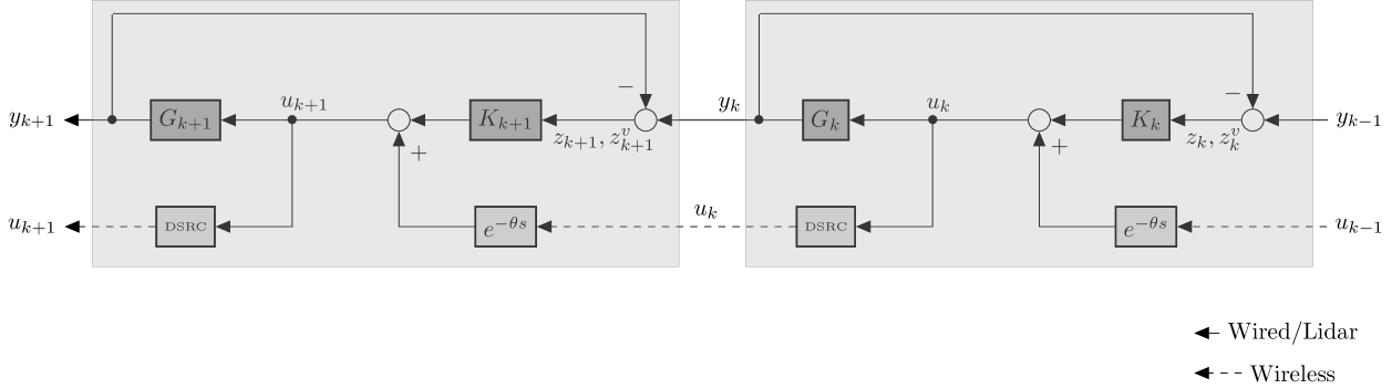
In Figure 1, we denoted with $K_{k}$ the input–output operator from $z_{k},z_{k}^{v}$ and $v_{k}$ respectively to $u_{k}^{\ell}$ of the $k$ -th sub-controller from (8), namely

u_{k}^{\ell}=K_{k}\star\big{(}z_{k},\>z_{k}^{v},\>v_{k}\big{)}.

(9)

The resulted control architecture for any two consecutive agents ( $k\geq 2$ ) can be pictured as in Figure 1. For all practical purposes, the existence of a time delay on each of the feedforward links $u_{k}$ , with $1\leq k\leq(n-1)$ must be taken into account. For readability, these time delays are figuratively denoted by $e^{-\theta s}$ in Figure 1 (the Laplace transform of a delay of $\theta$ seconds), representative to the situation in which the delayed version $u_{k}(t-\theta)$ version of the $u_{k}(t)$ signal is received on board of the $(k+1)$ agent. In applications, these delays are caused by the physical limitations of the wireless communications system used for the implementation of the feedforward link , entailing a $\theta$ time delay at the receiver. For automotive applications the standard digital radio communications systems (included in Figure 1) are DSRC¹⁰¹⁰10 IEEE 802.11p - Dedicated Short Range Communications.

Remark III.1

Without the assumption of inter-agent communications delays, one might argue that information from the leader propagates instantaneously to all the agents in formation, via a relay mechanism (from each agent to its successor) and consequently the resulted distributed scheme doesn’t employ local, but rather global information from the leader. It is known that precisely this type of time delays can drastically alter the performance control architectures based on such relay schemes [48].

Remark III.2

For the illustrative simplicity of the exposition, we look first at the scenario in which there are no time–delays induce by the inter-agent (wireless) communication of information, such as the predecessor’s control signal $u_{k-1}$ . A “synchronization” mechanism that can cope with the time-varying communications induced time–delays will be addressed in Section V.

III-A A First Glance at the Closed–Loop Dynamics Decoupling

The control policy (7) entails a highly beneficial “decoupling” feature of the closed–loop dynamics at each agent, as illustrated next. Firstly, note that by plugging (7) into (5) we obtain the following closed–loop error equations at the $k$ –th agent:

\dot{{z}}_{k}^{v}={{f}_{k-1}({v}_{k-1})-f_{k-1}}({v}_{k})-{\beta_{k}}{z}_{k}^{v}+\nabla_{{y}_{k}}V_{k,k-1}(\|z_{k}\|_{\sigma}).

(10)

The following result will be instrumental in the sequel. Consider the following Lyapunov candidate functions:

\begin{split}L_{k}\big{(}z_{k}(t),z_{k}^{v}(t)\big{)}\overset{def}{=}\frac{1}{2}\Big{(}V_{k,k-1}(\|{{z}}_{k}(t)\|_{\sigma})+\quad\quad\quad\quad\quad\quad\quad\\ \quad\quad\quad\quad\quad\quad\quad+{z}_{k}^{v}{}^{\top}(t){z}_{k}^{v}(t)\Big{)},\ \text{with}\;1\leq k\leq n.\end{split}

(11)

Lemma III.3

The derivative of the Lyapunov candidate function $L_{k}(\cdot,\cdot)$ introduced in (11) along the trajectories of (5) and (7) is given by

\begin{split}\frac{d}{dt}L_{k}(z_{k}(t),z_{k}^{v}(t))&={z}_{k}^{v}{}^{\top}(t)\Big{(}f_{k-1}\big{(}v_{k-1}(t)\big{)}-f_{k-1}\big{(}v_{k}(t)\big{)}\Big{)}\\ &\quad\quad\quad\quad\quad\quad\quad\quad-{\beta_{k}}{z}_{k}^{v}{}^{\top}(t){z}_{k}^{v}(t)\>,\end{split}

(12)

and does not depend on the choice of the APFs $V_{k,k-1}(\cdot)$ .

Proof:

Differentiating the APF $V_{k,k-1}(\cdot)$ at the $k$ –th agent with respect to time, yields

\begin{split}&\frac{d}{dt}V_{k,k-1}(\|{y}_{k-1}-{y}_{k}\|_{\sigma})={(\dot{{y}}_{k-1}-\dot{{y}}_{k})}^{\top}\times\\ &\big{(}\nabla_{{y}_{k-1}}V_{k,k-1}(\|{y}_{k-1}-{y}_{k}\|_{\sigma})-\nabla_{{y}_{k}}V_{k,k-1}(\|{y}_{k-1}-{y}_{k}\|_{\sigma})\big{)}\end{split}

(13)

and by employing the anti–symmetrical property of APFs [42, pp. 197] : $\nabla_{{y}_{k}}V_{k,k-1}(\|{z}_{k}\|_{\sigma})=-\nabla_{{y}_{k-1}}V_{k,k-1}(\|{z}_{k}\|_{\sigma})$ we get that

\frac{d}{dt}V_{k,k-1}(\|{z}_{k}\|_{\sigma})=-2\>{\dot{{z}}_{k}}{}^{\top}\>\nabla_{{y}_{k}}V_{k,k-1}(\|{z}_{k}\|_{\sigma}).

(14)

Therefore from (11) it follows that

\begin{split}\frac{d}{dt}L_{k}\big{(}z_{k}(t),z_{k}^{v}(t)\big{)}&={z}_{k}^{v}{}^{\top}\dot{{z}}_{k}^{v}-{z}_{k}^{v}{}^{\top}\nabla_{{y}_{k}}V_{k,k-1}(\|{z}_{k}\|_{\sigma})\\ &\hskip-34.14322pt={z}_{k}^{v}{}^{\top}\big{(}\dot{{z}}_{k}^{v}-\nabla_{{y}_{k}}V_{k,k-1}(\|{z}_{k}\|_{\sigma})\big{)}\\ &\hskip-34.14322pt\overset{(\ref{secundo})}{=}{z}_{k}^{v}{}^{\top}\big{(}{f}_{k-1}({v}_{k-1})-{f}_{k-1}({v}_{k}))-{\beta_{k}}{z}_{k}^{v}\big{)}\\ &\hskip-34.14322pt={z}_{k}^{v}{}^{\top}\big{(}{f}_{k-1}({v}_{k-1})-{f}_{k-1}({v}_{k})\big{)}-{\beta_{k}}{z}_{k}^{v}{}^{\top}{z}_{k}^{v}\end{split}

∎

IV Decoupling control design

The following result is the main result of this Section, as it delineates a “decoupling” property of the closed–loop dynamics, achieved by the type (7) control policy along with: (i) closed-loop stability, (ii) velocity matching, (iii) collision avoidance and (iv) formation topology preservation. Specifically, assuming that the acceleration of the leader vehicle becomes zero after a finite period of time (i.e. $v_{0}(t)$ reaches a steady-state) then the following theorem holds:

Theorem IV.1

If the functions $f_{k}(\cdot)$ with $0\leq k\leq n$ from (2a) satisfy the Lipshitz–like condition [42, Assumption 1]

\left|(v_{2}-v_{1})^{\top}\big{(}f_{k}(v_{2})-f_{k}(v_{1})\big{)}\right|\leq\alpha_{k}\|v_{2}-v_{1}\|_{2}^{2},\quad\forall\>v_{1},\>v_{2}

(15)

then for any of the type (7) control laws, such that $\beta_{k}>\alpha_{k-1}$ , the following hold:

(A) Given the Lyapunov function $L_{k}(\cdot,\cdot)$ from (11), local to the $k$ -th agent, then for any real constant $c>0$ the sub–level sets $\Omega_{c}^{k}\overset{def}{=}\{(z_{k},z_{k}^{v})|L_{k}(z_{k},z_{k}^{v})\leq c\}$ of $L_{k}(\cdot,\cdot)$ are compact and they represent forward invariant sets for the local closed–loop dynamics (10) of the $k$ –th agent.
(B) The control laws (7) guarantee velocity matching in the steady-state i.e. $\displaystyle\lim_{t\rightarrow\infty}\|z_{k}^{v}(t)\|=0$ and collision avoidance in the transient regime, i.e. there exists $\eta_{c}>0$ such that

\|z_{k}(t)\|_{2}>\eta_{c},\;\forall t\geq 0.

\lim_{t\rightarrow\infty}\|z_{k}(t)\|_{2}=\delta_{k}

where $\delta_{k}$ is a pre-specified real, positive value.

Proof:

(A) We show that for any real $c>0$ the local sub–level sets $\Omega_{c}^{k}\overset{def}{=}\{(z_{k},z_{k}^{v})|\ L_{k}(z_{k},z_{k}^{v})\leq c\}$ of $L_{k}(\cdot,\cdot)$ are compact. Note that $L_{k}(z_{k},z_{k}^{v})<c$ implies that $\|{z}_{k}^{v}\|<2c$ and $V_{k,k-1}(\|z_{k}\|_{\sigma})<2c$ . Since $V_{k,k-1}(\cdot)$ is radially unbounded this implies that $\|z_{k}\|_{\sigma}$ is bounded and consequently $\|z_{k}\|_{2}$ is bounded. Therefore $\Omega_{c}^{k}\subset{\bf R}^{2\text{dim}(y_{k})}$ is a bounded set¹¹¹¹11Here $\text{dim}(y_{k})$ denotes the dimension of the $y_{k}(t)$ vector valued function of time, which in general may be greater than one.. Moreover due to the continuity of $\|\cdot\|_{\sigma}$ and of $L_{k}(\cdot)$ , one obtains that $\Omega_{c}^{k}$ is a closed set. Precisely $\Omega_{c}^{k}$ is the pre-image of a closed set through a continuous function. In the Banach space ${\bf R}^{2\text{dim}(y_{k})}$ it therefore holds that $\Omega_{c}^{k}$ is closed and bounded thus $\Omega_{c}^{k}$ is compact. Furthermore, Lemma III.3 and the Lipschitz–like assumption (15) on all $f_{k}(\cdot)$ implies that

\frac{d}{dt}L_{k}\big{(}z_{k}(t),z_{k}^{v}(t)\big{)}\leq(\alpha_{k-1}-\beta_{k}){z}_{k}^{v}{}^{\top}(t){z}_{k}^{v}(t),\ \forall k

along the trajectories of (10). Therefore it suffices to choose the controller gain $\beta_{k}>\alpha_{k-1}$ in order to guarantee that along the trajectories of (10) it holds that $\displaystyle\frac{d}{dt}L_{k}\big{(}z_{k}(t),z_{k}^{v}(t)\big{)}<0$ and also that $\displaystyle\Omega_{c}^{k}$ is a forward invariant set for the “decoupled” closed–loop system (10), local to the $k$ -th agent.

(B) From the properties of the APF (Definition II.3) it follows that $V_{k,k-1}(\|z_{k}\|_{\sigma})\rightarrow\infty$ as $\|z_{k}\|_{2}\rightarrow 0$ , i.e. $\forall c>0,\ \exists\eta_{c}>0$ such that

V_{k,k-1}(\|z_{k}\|_{\sigma})>c,\ \forall\ \|z_{k}\|_{2}<\eta_{c}.

(16)

Let $c_{k}=\min_{r\geq 0}V_{k,k-1}(r)>0$ . It follows from (16) that for any positive $c>c_{k}$ one has that

V_{k,k-1}(\|z_{k}\|_{\sigma})\leq c\mbox{ implies }\|z_{k}\|_{2}\geq\eta_{c}.

(17)

Note that an increase of $c$ is correlated with a corresponding decrease of $\eta_{c}$ . Next, let us fix $c=2L_{k}(z_{k}(0),z_{k}^{v}(0))$ . From point (A) above it follows that for $\beta_{k}>\alpha_{k-1}$ it holds that $\Omega_{c}^{k}$ is a forward invariant set with respect to (10) and consequently $L_{k}(z_{k}(t),z_{k}^{v}(t))\leq\frac{c}{2},\ \forall t\geq 0$ . This implies via (11) that $V_{k,k-1}(\|z_{k}(t)\|_{\sigma})<c,\ \forall t\geq 0$ which in turn yields $c>c_{k}$ and so from (16) we conclude that

\|z_{k}\|_{2}>\eta_{c},\ \forall t\geq 0.

It is noteworthy that $\eta_{c}$ is implicitly defined by $c$ which in turn depends on the initial conditions $(z_{k}(0),z_{k}^{v}(0))$ .

(C) Given $L_{k}(\cdot,\cdot)$ as introduced in (11), it is claimed that the string formation’s steady–state configuration is attained at the minimum of the following formation-level Lyapunov function, defined as

L(z(t),z^{v}(t))\overset{def}{=}\frac{1}{2}\sum_{k=1}^{n}L_{k}(z_{k}(t),z_{k}^{v}(t))

(18)

where $z(t),z^{v}(t)$ are the aggregated vectors of the regulated measurements for the entire formation, obtained by adequately stacking the local measurements $z_{k}(t),z_{k}^{v}(t)$ of the agents:

z(t)\overset{def}{=}\left[\begin{array}[]{cccc}z_{1}(t)&z_{2}(t)&\dots&z_{n}(t)\end{array}\right]^{\top}

(19)

z^{v}(t)\overset{def}{=}\left[\begin{array}[]{cccc}z_{1}^{v}(t)&z_{2}^{v}(t)&\dots&z_{n}^{v}(t)\end{array}\right]^{\top}

(20)

The minimum of (18) therefore coincides (component–wise) with the minima of the Lyapunov functions (11) local to the $k$ -th agent.

In order to prove the claim, first note that the level sets of $L(\cdot,\cdot)$ given by $\Omega_{c}\overset{def}{=}\{(z,z^{v})|L(z,z^{v})\leq c,\;\text{with}\>c>0\}$ are compact, since $\Omega_{c}$ is a finite cartesian product of the $\Omega_{c}^{k}$ sets, whose compactness was proved at point (B) above. By a similar argument, it follows that $\Omega_{c}$ represents a forward invariant set for the closed–loop dynamics of the entire formation, along the trajectories of (10), where $1\leq k\leq n$ .

Note that from the definition of (18) and Lemma III.3 that along the trajectories of (2) and (7) one has that

\begin{split}\frac{d}{dt}L\big{(}z(t),z^{v}(t)\big{)}=\quad\quad\quad\quad\quad\quad\quad\quad\quad\quad\quad\quad\quad\quad\quad\quad\\ \quad\quad\quad\sum_{k=1}^{N}{z}_{k}^{v}{}^{\top}\Big{(}{f}_{k-1}({v}_{k})-{f}_{k-1}(({v}_{k-1})\Big{)}-\sum_{k=1}^{N}{\beta_{k}}{z}_{k}^{v}{}^{\top}{z}_{k}^{v}\>.\end{split}

(21)

Therefore, by employing LaSalle’s invariance principle we conclude that the Lyapunov function $L_{k}(z_{k}(t),z_{k}^{v}(t))$ converges asymptotically to its minimum i.e. $\frac{d}{dt}L_{k}\big{(}z_{k}(t),z_{k}^{v}(t)\big{)}=0$ , which is attained at velocity matching as $z_{k}^{v}=0$ (or equivalently when $v_{k-1}=v_{k}$ ) . Denote with $(\delta_{k},0)$ the point at which such minimum is attained and note that $\delta_{k}>0$ by the collision avoidance attribute from point (B). Consequently, in the steady-state $\|z_{k}^{v}(t)\|_{2}$ converges to $0$ , while $\|z_{k}(t)\|_{2}$ converges to $\delta_{k}$ and the formation’s topology preservation

\lim_{t\rightarrow\infty}\|z_{k}(t)\|_{2}=\delta_{k},\quad 1\leq k\leq n,

is guaranteed. ∎

Remark IV.2

The pre-specified positive constants $\delta_{k}$ (with $1\leq k\leq n$ ) representing the desired steady-state inter-agent distances, can be integrated in the Lyapunov functions $L_{k}(\cdot,\cdot)$ at the controller design stage, as exemplified in Section VI.

IV-A Communicating the Control Signals of the sub-Controllers

When looking at the problem of agents moving in the string formation, the intuition behind the type (7) control law is that it essentially includes an implementation of the common “break lamp bulb” regulated in all road traffic. This is the conceptual difference of the proposed distributed architecture: instead of choosing to communicate the regulated measurements between sub-controllers (as done in the cooperative output regulation setup such as [33, 34, 35, 36]) the sub-controllers choose to transmit their control actions. This feature turns out to be essential in achieving the synchronization objective along with all the other standard performance requirements (e.g. collision avoidance, topology preservation) from displacement-based formation control [40, Section 6], as outlined by the following result.

Proposition IV.3

If the predecessor’s control action $u_{k-1}(t)$ is not made available at the $k$ -th agent in the controller equation (7) then velocity matching cannot be attained.

Proof:

We prove the result by contradiction. Let us assume that velocity matching is achieved. Consequently, in the steady-state $\|{z}_{k}^{v}(t)\|_{2}$ converges to zero and $\|{z}_{k}(t)\|_{\sigma}$ converges to some constant $\eta\geq\delta_{k}$ . Since $V_{k,k-1}(\cdot)$ is a class $C^{1}$ function, all its partial derivatives are continuous and so $\nabla_{{y}_{k}}V_{k,k-1}(\|z_{k}\|_{\sigma})$ converges to a vector

\nabla_{\eta}\overset{def}{=}\nabla_{{y}_{k}}V_{k,k-1}(\|z_{k}\|_{\sigma})\big{|}_{\|{z}_{k}(t)\|_{\sigma}=\eta}

Whenever $\|{z}_{k}^{v}(t)\|_{2}$ converges to zero, it follows that

\forall c>0,\ \exists\ t_{0}>0\mbox{ such that }\|{z}_{k}^{v}(t)\|_{2}\leq c,\ \forall t\geq t_{0}.

(22)

In order to show that (22) is violated, let $c>0$ be fixed and $t_{0}=\max\{t>0\mid\|{z}_{k}^{v}(t)\|_{2}=c\}$ . Therefore, we should have $\|{z}_{k}^{v}(t)\|_{2}<c,\ \forall t\geq t_{0}$ .
Since $\nabla_{{y}_{k}}V_{k,k-1}(\|z_{k}\|_{\sigma})$ converges to $\nabla_{\eta}$ one has that $\exists\epsilon>0$ such that

\big{|}{z}_{k}^{v}{}^{\top}(t)\big{(}\nabla_{{y}_{k}}V_{k,k-1}(\|z_{k}\|_{\sigma})-\nabla_{\eta}\big{)}\big{|}<\epsilon c

Employing (15) (while noting that $u_{k-1}$ is implicitly present in the closed-loop equations (10)), one obtains:

\begin{split}&\frac{d}{dt}\|{z}_{k}^{v}(t)\|_{2}={z}_{k}^{v}{}^{\top}(t)\Big{(}f_{k-1}\big{(}v_{k-1}(t)\big{)}-f_{k-1}\big{(}v_{k}(t)\big{)}\Big{)}\\ &-{\beta_{k}}{z}_{k}^{v}{}^{\top}(t){z}_{k}^{v}(t)+{z}_{k}^{v}{}^{\top}(t)\nabla_{{y}_{k}}V_{k,k-1}(\|z_{k}\|_{\sigma})\\ &+{z}_{k}^{v}{}^{\top}(t)u_{k-1}(t)\>\\ &\geq-(\alpha_{k-1}+\beta_{k}){z}_{k}^{v}{}^{\top}(t){z}_{k}^{v}(t)-\epsilon c+{z}_{k}^{v}{}^{\top}(t)\big{(}\nabla_{\eta}+u_{k-1}(t)\big{)}\>.\end{split}

Therefore, while

u_{k-1}(t)=(\beta_{k}+\alpha_{k-1}+2\epsilon){z}_{k}^{v}(t)-\nabla_{\eta}

(23)

it follows that $\displaystyle\frac{d}{dt}\|{z}_{k}^{v}(t_{0})\|_{2}>0$ which in turn implies that (22) doesn’t hold. It is important to note here that no increase in the control effort by choosing a larger gain $\beta_{k}$ can help in achieving velocity matching, since for arbitrarily large but finite values of $\beta_{k}$ , under the assumption that $\|{z}_{k}^{v}(t)\|_{2}$ converges to zero, one gets that the term $(\beta_{k}+\alpha_{k-1}+2\epsilon){z}_{k}^{v}(t)$ becomes arbitrarily small. Nevertheless, once this term becomes small, there always exists a bounded contro input $u_{k-1}$ of the form (23) that precludes $\|{z}_{k}^{v}(t)\|_{2}$ from converging to zero. ∎

IV-B Some Considerations and Future Work

For illustrative simplicity, we provide below an informal outlook of our approach leading to the proposed distributed controller architecture for the string network. We look at how the aggregated variables for the entire formation relate to the agents’ individual variables (the states - including the absolute coordinates $y_{k}$ and the speeds $v_{k}$ , the sub-controller’s outputs $u_{k}$ and the measurements $z_{k},z_{k}^{v}$ local to the $k$ -th agent) . Let us define:

v(t)\overset{def}{=}\left[\begin{array}[]{cccc}v_{0}(t)&v_{1}(t)&\dots&v_{n}(t)\end{array}\right]^{\top}

(24)

u(t)\overset{def}{=}\left[\begin{array}[]{cccc}u_{0}(t)&u_{1}(t)&\dots&u_{n}(t)\end{array}\right]^{\top}

(25)

f\big{(}v(t)\big{)}\overset{def}{=}\left[\begin{array}[]{cccc}f_{0}(u_{0})&f_{1}(u_{1})&\dots&f_{n}(u_{n})\end{array}\right]^{\top}

(26)

while the vectors of the aggregated measurements $(z,z^{v})$ have been introduced in (19), (20). The aggregated equations (2a) for the entire formation become

\dfrac{d}{dt}{{v}}(t)=f({v}(t))+{u}(t)

(27)

The objective of the control scheme is related to the regulated measurements (in our case $z^{v}$ ), which (in general) are functions of the agent’s states (in our case $v$ ). Let us describe this dependence by

z^{v}=\mathcal{J}(v)

(28)

In many situations of practical interest the $\mathcal{J}(\cdot)$ operator may be linear. For the situation studied here, it follows from (4) that $\mathcal{J}(\cdot)$ is an $n\times(n+1)$ real matrix having entries equal to “ $1$ ” on its diagonal and “ $-1$ ” on its supra-diagonal. In displacement-based formation control the type (28) definition of the regulated variables (e.g. relative distances or relative speeds) encapsulates the topology of the multi-agent formation. In related formulations (e.g. the optimal control formulation for LTI agents from [25]) the $\mathcal{J}(\cdot)$ operator may also enclose norm based costs.

Let us assume next that $\mathcal{J}(\cdot)$ commutes with the differentiating operator $\displaystyle d/dt$ and apply $\mathcal{J}(\cdot)$ to both sides of (27), while taking into account its linearity and the definition of the regulated variables (28) in order to get

\dfrac{d}{dt}\mathcal{J}(v(t))=\mathcal{J}\Big{(}f({v}(t))\Big{)}+\mathcal{J}\Big{(}{u}(t)\Big{)}

(29)

The merit of the type (29) formulation is that it is expressed directly in terms of the regulated measurements $z^{v}=\mathcal{J}(v)$ (on the left-hand side) and not of the original states $v$ from (27), while the dynamics of “the plant” have changed from $f(\cdot)$ to $\mathcal{J}(f(\cdot))$ . The morale is that the distributed controller design may now be performed on (29) in order to obtain the control laws $\mathcal{J}(u)$ . This is exactly the approach taken for the string formation, where for the regulated measurements $z_{k}^{v}=v_{k-1}-v_{k}$ we have essentially performed a decentralized controller synthesis (6) for the control signals $(u_{k-1}-u_{k})$ . The relation from (29) also suggests that the sub-controller communications topology should “borrow” the formation’s topology. This entails the “dynamic decoupling” attained by the string formation, the existence of “local” forward invariant sets and Lyapunov functions and the possibility of performing independent regulation and sub-controller design at each agent.

Finding suitable distributed controllers for more general types of $\mathcal{J}(\cdot)$ operators is the objective of future investigations. Assuming that the distributed controller design for (29) successfully yields the control laws $\mathcal{J}(u)$ , there still remains the problem of finding a causal implementation of such a controller¹²¹²12This aspect will appear even more more clearly in those formulations of these type of problems involving dynamical systems with discrete-time. in terms of the $u$ signals of the original formulation (27). This may require certain invertibility assumptions on the $\mathcal{J}(\cdot)$ mapping. Furthermore, looking at any practical implementation of the proposed law from (7), the local control $u_{k}(t)$ should only depend on the delayed version of $u_{k-1}(t)$ (or on its history). These important issues will be discussed in Section V below.

IV-C Platooning Control

Platooning control has been a longstanding problem in control engineering, encompassing a vast literature. For a series of recent, interesting results also providing a good outline of existing literature we refer to [49, 50]. To the best of the authors’s knowledge, the current results are the only ones guaranteeing collision avoidance and topology preservation for heterogenous, nonlinear dynamical agents in the presence of communication induced time-delays, as outlinen in Section V below. In this context, the current paper can be looked at as an extension to nonlinear control of the novel ideas for $\mathcal{H}_{2}/\mathcal{H}_{\infty}$ control of LTI agents in [25].

V A Practical Time-Delays Compensation Mechanism

The difficulties caused for networked systems by the communications induced delays and time jittering have been a topic of intensive study for decades. In formation control practical applications it has been argued in [48] that the (relatively low latency) time delays induced by the wireless communications of the control signals $u_{k}$ from one agent to its successor in the string (even if assumed time-invariant and homogeneous¹³¹³13For digital radio wireless systems such as WiFi, Bluetooth or Zigbee, the corresponding time-delays have low latencies but they are time-varying, taking values around a nominal delay of about 20 ms.) irremediably alter the performance of the control scheme. What happens is that the delays propagate through the closed-loops towards the back of the platoon where they “accumulate” in a manner depending on the number of vehicles in formation [48].

For the case of LTI dynamical agents, the very recent results from [25] provide a functional solution for compensating the effect of the communications delays by introducing (with high accuracy) supplemental delays at key points in the closed loop. However, the aforementioned method [25, Section VI] of essentially “moving” the synchronization delay through the loop and ultimately incorporating it in the model of the “plant” cannot be directly adapted to nonlinear dynamical systems. In this section we show how an adaptation of the distributed controller of Section IV is able to compensate the communications delays, while essentially preserving all the performance features from the delay free case. The approach taken here is based on: (i) the tailored use of the so-called time-headways without sacrificing the tightness of the formation and (ii) changing the definition of regulated measurements to a meaningful approximation. The main challenge here is for the re-defined regulated measurements to remain measurable (on board of each agent) in a distributed manner.

V-A Adapting Time-Headways for Delays Compensation

Classical results in platooning control [51, 52, 53] proved that a considerable improvement of performance can be obtained by adequately modifying the regulated interspacing distance (for each vehicle $k$ ) $z_{k}=y_{k-1}-y_{k}$ such as to include a factor $-h\dot{y}_{k}(t)$ proportional with the speed of the current vehicle. The resulted interspacing policies (dubbed time-headways) become $z_{k}=y_{k-1}(t)-y_{k}(t)-h\dot{y}_{k}(t)$ (where $h>0$ , the so called time-headway, is a real, positive constant) and provide a spacing in time rather than distance (between two consecutive vehicles). Up until the recent distributed scheme introduced in [25] - in the case of LTI dynamical agents - good attenuation at all frequencies could only be achieved via the use of time headways policies [54]. The generally adopted value for highway platooning (which became the standard at some point) is $h=1$ second. The main drawback of such large time headways is that they destroy the tightness of the formation, drastically reducing the highway traffic throughput or any potential fuel savings achievable by the air drag reduction.

We introduce next a novel method for delays compensation that combines the synchronized-clocks mechanism from [25, Section VI] with an adequate adaptation of the time headways. Firstly, let us revamp as follows the definitions (4) of the interspacing distances $z_{k}$ and of the regulated relative speeds $z_{k}^{v}$ respectively at the $k$ -th vehicle:

\begin{split}&{{\widetilde{z}}}_{k}(t)\overset{def}{=}{y}_{k-1}(t-\theta)-{y}_{k}(t-\theta)-\theta\dot{y}_{k}(t-\theta),\\ &{{\widetilde{z}}}_{k}^{v}(t)\overset{def}{=}{v}_{k-1}(t-\theta)-{v}_{k}(t-\theta)-\theta\dot{v}_{k}(t-\theta),1\leq k\leq n,\\ \end{split}

(30)

where the positive constant $\theta>0$ , i.e. the time-headway, will be taken to be equal with the communications delay and will be considered (without any loss of generality) to be the same for all vehicles in formation¹⁴¹⁴14See also Remark V.1 below. It can be seen that the signals defined in (30) are merely $\theta$ delayed version of (4) with a $\theta$ time-headway.

If at the current moment in time $t$ , we would choose to regulate instead the measurements taken at moment $(t-\theta)$ according to (30), that would be a limitation imposed by the communications delay (which are relatively very small, though) and it would entail some loss in performance which was to be expected. The inclusion of the $\theta$ time headway results in a slightly more conservative policy, since it induces slightly larger interspacing distances as the speed increases. The same conservative effect (of the $\theta$ time headway) occurs with respect to the regulated relative speeds ${{\widetilde{z}}}_{k}^{v}(t)$ during the transient regime when the acceleration $\dot{v}_{k}$ is sizable.

Remark V.1

For all practical applications related to platooning, the value of $\theta$ will be taken to be equal to a worst case scenario value of the latency of the wireless communication systems, which is about $2\times 10^{-2}$ seconds for digital radio systems such as DSRC, WiFi, Bluetooth or Zigbee. Furthermore, the “synchronized clocks” mechanism introduced in [25, Section VI] used in conjunction with time stamping protocols (at the transmission of the predecessor’s control signal $u_{k-1}$ ) is able to emulate and implement time invariant and heterogeneous communications time delays throughout the entire formation, by introducing with high accuracy supplemental delays in the closed-loop.

Remark V.2

The effect of the time-headway on the behavior of the formation is directly proportional with the numerical value of $\theta$ , which is very small in practice¹⁵¹⁵15See Remark V.1 above.. In fact, for formation control practical applications the effect is almost negligible given the order of magnitude of $\theta$ compared to the time constants of the dynamics of road or aerial agents.

V-B Changing the Regulated Measurements

In the next proposition we re-define the regulated measurements and make the express remark that the definition included below will be enforced onward, throughout the contents of the current Section V.

Proposition V.3

We assume the following initial conditions

y_{k}(t)=-\sum_{j=0}^{k}\ell_{j},\quad v_{k}(t)=0,\ \forall t\in(-\theta,0],

and further define the regulated measurements to be:

\begin{split}&{{z}}_{k}(t)\overset{def}{=}{y}_{k-1}(t-\theta)-{y}_{k}(t)\\ &{{z}}_{k}^{v}(t)\overset{def}{=}{v}_{k-1}(t-\theta)-{v}_{k}(t)\quad\text{for}\quad 1\leq k\leq n.\end{split}

(31)

It follows that ${{z}}_{k}(t),{{z}}_{k}^{v}(t)$ from (31) above represent an $\mathcal{O}(\theta^{2})$ approximation of ${{\widetilde{z}}}_{k}(t)$ and ${{\widetilde{z}}}_{k}^{v}(t)$ respectively, from (30).

Proof:

It follows by the very definition of (31) and (30) respectively and the following Taylor series expansion:

\begin{split}&{y}_{k}(t)={y}_{k}(t-\theta)+\theta\dot{y}_{k}(t-\theta)+\mathcal{O}(\theta^{2}),\\ &{v}_{k}(t)={v}_{k}(t-\theta)+\theta\dot{v}_{k}(t-\theta)+\mathcal{O}(\theta^{2}).\end{split}

(32)

∎

Remark V.4

One essential practical issue is to establish if the new regulated signals (31) remain measurable on board of the $k$ -th agent (in a distributed manner). Writing in (31) the Taylor series expansion with an integral rest for $y_{k}(t)$ and $v_{k}(t)$ respectively, we obtain the following equivalent expressions:

\begin{split}&{{z}}_{k}(t)\overset{}{=}{y}_{k-1}(t-\theta)-{y}_{k}(t-\theta)-\int_{t-\theta}^{t}\dot{y}_{k}(\tau)d\tau,\\ &{{z}}_{k}^{v}(t)\overset{}{=}{v}_{k-1}(t-\theta)-{v}_{k}(t-\theta)-\int_{t-\theta}^{t}\dot{v}_{k}(\tau)d\tau\end{split}

(33)

or equivalently

\begin{split}&{{z}}_{k}(t)\overset{}{=}{z}_{k}(t-\theta)-\int_{t-\theta}^{t}v_{k}(\tau)d\tau,\\ &{{z}}_{k}^{v}(t)\overset{}{=}{z_{k}^{v}}(t-\theta)-v_{k}(t)+v_{k}(t-\theta)\end{split}

(34)

and so it becomes apparent that the signals introduced in (31) can be measured on board the $k$ -th vehicle via (34), using only onboard ranging sensors¹⁶¹⁶16Preferably very low latency LIDAR sensors, which are already affordable and widely available commercially and high accuracy longitudinal speedometers in conjunction with a mere integrator. Specifically, the first term in (34) consists of the $\theta$ -delayed measurement of the interspacing distance minus the integration of the absolute speed (measurable on board) over a $\theta$ -length interval. The second term in (34) consists of the $\theta$ -delayed measurement of the relative speed¹⁷¹⁷17The relative speed with respect to the preceding vehicle, which is also measurable onboard, see also footnote number 9 on page four. minus the $(v_{k}(t)-v_{k}(t-\theta))$ term, comprised of absolute speeds measurable onboard the $k$ agent. Finally, the entire history on the interval $[(t-\theta),\;t]$ of the ranging sensors (34) must be stored in a memory buffer, in order to be used by the distributed controller we will introduce next.

The following remark represents the conclusion of the current Subsection V-B:

Remark V.5

Given the values of $\theta$ that appear in practice (see Remark V.1) and given the worst case scenario of breaking decelerations $|\dot{v}_{k}(t)|$ that could occur during highway traffic, it follows via Proposition V.3 that the signals from (31) are such an accurate approximation of (34), that the order of the approximation falls way below the tolerated measurement errors of the most performant ranging sensors. That is to say that choosing between two controllers that regulate either the (30) signals or the (34) signals respectively, has considerably less influence on the resulted scheme than the measurement noise of an highly accurate LIDAR. Consequently, in the scheme proposed next, we choose to regulate (34).

V-C A Controller to Cope with Time Delays

Considering the definition of $z_{k}$ and $z_{k}^{v}$ as in (31), we will prove that the distributed control policies given next are able to entirely compensate the communication induced delays:

\left\{\begin{split}{u}_{k}(t)=&{u}_{k-1}(t-\theta)+{\beta_{k}}{{z}}_{k}^{v}(t)+\nabla_{{y}_{k}}V_{k,k-1}(\|{{z}}_{k}(t)\|_{\sigma})\\ -&{f}_{k}({v}_{k})+{f}_{k-1}({v}_{k})\\ {u}_{k}(t)=&0,\quad\forall t\in(-\theta,0]\end{split}\right.

(35)

Remark V.6

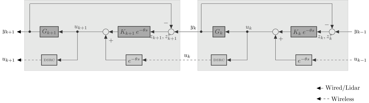
Note that for the real time, practical implementation of type (35) control policies onboard the $k$ -th vehicle, two pieces of information are needed: (i) the command signal ${u}_{k-1}(t-\theta)$ of the predecessor, received on board via (DRSC) wireless communications with a $\theta$ -delay and (ii) the (34) sensor measurements $z_{k},z_{k}^{v}$ , which are measurable on board the $k$ -th agent, as per the considerations from Remark V.4. Note that in order for the scheme to be effective, the $\theta$ communications delay from ${u}_{k-1}(t-\theta)$ must be replicated with high accuracy in the in $z_{k}(t),z_{k}^{v}(t)$ measurements from (34). This resembles the (GPS time-base) synchronization mechanism in [25, Section VI]) for the LTI case and it can be implemented using time-stamping protocols of the involved signals ${u}_{k-1}$ and $z_{k}(t),z_{k}^{v}(t)$ . In Figure 2, such $\theta$ “synchronization” delays to be imposed on the $z_{k}(t),z_{k}^{v}(t)$ signals from (34) have been figuratively incorporated in the controller, via the $e^{-\theta s}$ term. The aforementioned synchronization will ensure time invariant, point-wise delays of value exactly $\theta$ , homogeneously throughout the entire formation as per the considerations from Remark V.1.

We employ the Lyapunov function from (11) keeping in mind that the definitions of ${{z}}_{k}(t),{{z}}_{k}^{v}(t)$ are in accordance to (31). Specifically, assuming that the acceleration of the leader vehicle becomes zero after a finite period of time (i.e. $v_{0}(t)$ reaches a steady-state), the time delays adaptation for the main result of Section IV reads:

Theorem V.7

If the function $f(\cdot)$ from (2a) satisfies the global Lipshitz–like condition (15) then for any of the type (35) control laws, such that $\beta_{k}>\alpha_{k-1}$ the following hold:
(A) The derivative of the Lyapunov candidate function $L_{k}(\cdot,\cdot)$ from (11), local to the $k$ -th agent, along the trajectories of (5) and (35) is given by

\begin{split}&\frac{d}{dt}L_{k}(z_{k}(t),z_{k}^{v}(t))=-{\beta_{k}}{z}_{k}^{v}{}^{\top}(t){z}_{k}^{v}(t)+\\ &\qquad{z}_{k}^{v}{}^{\top}(t)\Big{(}f_{k-1}\big{(}v_{k-1}(t-\theta)\big{)}-f_{k-1}\big{(}v_{k}(t)\big{)}\Big{)}\>,\end{split}

(36)

and does not depend on the choice of the APFs $V_{k,k-1}(\cdot)$ .
(B) Given the Lyapunov function $L_{k}(\cdot,\cdot)$ from (11), local to the $k$ -th agent, the sub–level sets $\Omega_{c}^{k}\overset{def}{=}\{(z_{k},z_{k}^{v})|L_{k}\leq c,\;\text{with}\>c>0\}$ of $L_{k}$ are compact and they represent forward invariant sets for the local closed–loop dynamics of the $k$ –th vehicle.
(C) The control laws (35) guarantee velocity matching in the steady-state i.e. $\displaystyle\lim_{t\rightarrow\infty}\|z_{k}^{v}(t)\|=0$ and collision avoidance in the transient regime, i.e. there exists $\eta_{c}>0$ such that

\|z_{k}(t)\|_{2}>\eta_{c},\;\forall t\geq 0.

The controller (35) also guarantees the formation’s topology preservation in the steady-state, i.e.

\lim_{t\rightarrow\infty}\|z_{k}(t)\|_{2}=\delta_{k}

where $\delta_{k}$ is a pre-specified real, positive value.

Proof:

(A) With the controller (35) at hand we obtain the following closed–loop equations at the $k$ –th agent:

\begin{split}\dot{{z}}_{k}^{v}(t)&={{f}_{k-1}({v}_{k-1}(t-\theta))-f_{k-1}}({v}_{k}(t))\\ &-{\beta_{k}}{z}_{k}^{v}(t)+\nabla_{{y}_{k}}V_{k,k-1}(\|z_{k}(t)\|_{\sigma}).\end{split}

(37)

Let us notice that we deal with one fixed delay. Therefore, its derivative is 0 and consequently no complexity is added to the computations with respect to the proof of Lemma III.3. One straightforwardly gets that

\frac{d}{dt}V_{k,k-1}(\|{z}_{k}\|_{\sigma})=-2\>{\dot{{z}}_{k}}{}^{\top}\>\nabla_{{y}_{k}}V_{k,k-1}(\|{z}_{k}\|_{\sigma})

with ${z}_{k}$ as defined in (31). Since $\dot{{z}}_{k}={z}_{k}^{v}$ it follows that

\begin{split}&\frac{d}{dt}L_{k}(z_{k}(t),z_{k}^{v}(t))=-{\beta_{k}}{z}_{k}^{v}{}^{\top}(t){z}_{k}^{v}(t)+\\ &\qquad{z}_{k}^{v}{}^{\top}(t)\Big{(}f_{k-1}\big{(}v_{k-1}(t-\theta)\big{)}-f_{k-1}\big{(}v_{k}(t)\big{)}\Big{)}\>,\end{split}

(B) Notice that since $f_{k-1}(\cdot)$ satisfies (15) it follows that

\begin{split}{z}_{k}^{v}{}^{\top}(t)\Big{(}f_{k-1}\big{(}v_{k-1}(t-\theta)\big{)}-f_{k-1}\big{(}v_{k}(t)\big{)}\Big{)}\leq\\ \alpha_{k-1}{z}_{k}^{v}{}^{\top}(t){z}_{k}^{v}(t)\end{split}

Consequently, along the trajectories of the closed-loop system (37) one has

\frac{d}{dt}L_{k}(z_{k}(t),z_{k}^{v}(t))\leq(\alpha_{k-1}-\beta_{k}){z}_{k}^{v}{}^{\top}(t){z}_{k}^{v}(t).

Choosing $\beta_{k}>\alpha$ we guarantee that $\frac{d}{dt}L_{k}(z_{k}(t),z_{k}^{v}(t))<0$ along the trajectory of (37). Moreover, it follows along the lines of the proof of Theorem IV.1 that $\Omega_{c}^{k}$ is compact and forward invariant.
(C) Along the lines of the proofs of points (B) and (C) of Theorem IV.1 we can show that there exists $\eta>0$ such that

\|{z}_{k}\|_{2}>\eta,\quad\forall t\geq 0

and the steady state value is given by

\lim_{t\rightarrow\infty}\|{z}_{k}(t)\|_{2}=\delta_{k}.

In order to obtain the desired results we have just to notice that for all $k$ the function ${y}_{k-1}(t)$ is non-decreasing in time. Consequently,

\|{y}_{k}(t)-{y}_{k-1}(t)\|_{2}\geq\|{y}_{k}(t)-{y}_{k-1}(t-\theta)\|_{2}>\eta,\ \forall t>0

and

\lim_{t\rightarrow\infty}\|{y}_{k}(t)-{y}_{k-1}(t)\|_{2}\geq\lim_{t\rightarrow\infty}\|{z}_{k}(t)\|_{2}=\delta_{k}

∎

Remark V.8

The scheme proposed above is able to regulate ${v}_{k-1}(t-\theta)-{v}_{k}(t)$ in the presence of communications delays. Therefore, as far as the leader’s velocity profile is slowly varying relatively to the order of magnitude of the communications delays, the scheme does regulate an accurate approximation of ${v}_{k-1}(t)-{v}_{k}(t)$ . Nevertheless, oscillations of the leader’s velocity at a frequency that is of the same order of magnitude with $1/\theta$ , cannot be efficiently compensated and the accordion effect will appear. These assumptions are very well satisfied in the platooning setting, but they may not be valid for other applications. The conclusion is in line with the well known fact that for the validity of the control scheme it is always necessary that the time delays that propagate through the controller are smaller than those propagating through the given plant.

VI A Numerical Example and Further Considerations

In this section we illustrate the distributed controllers introduced above for dynamical agents (2) where the function $f_{k}(\cdot)$ has a quadratic form $f_{k}(v)=-\gamma_{k}g-\ell_{k}v^{2}$ , in accordance with the dynamical model of road vehicles from [55, (1)/pp. 1]. Here, $g=9.81\>m/s^{2}$ is the gravitational acceleration, $\gamma_{k}$ is the tyre rolling resistance coefficient and $\ell_{k}$ the air drag constant of vehicle $k$ . The dynamics (2) are

	$\dot{y}_{k}=v_{k}$		(38a)
	$\dot{v}_{k}=-\gamma_{k}g-\ell_{k}v_{k}^{2}+\frac{\eta}{R}w_{k}$		(38b)

with $\eta$ the gear ratio and $R$ the wheel radius. The command signal $\omega_{k}$ is the engine’s torque, and its linear transformation $\frac{\eta}{R}\omega_{k}$ corresponds to the input $u_{k}$ in (2). We take the same values for $\eta=1.8$ and $R=0.5$ across all the vehicles, to preserve the same meaning of the input $u$ . Note that for bounded velocities $|v_{1}|,|v_{2}|\leq v_{\max}$ , $f_{k}(\cdot)$ in (38) satisfies the Lipschitz–like condition [42, Assumption 1] $(v_{2}-v_{1})^{\top}\big{(}f_{k}(v_{2})-f_{k}(v_{1})\big{)}\leq\alpha_{k}|v_{2}-v_{1}|^{2}$ , with $\alpha_{k}=2\ell_{k}v_{\max}$ . We take $v_{\max}=60$ m/s (i.e. 216 km/h) in our experiments.

The control law is designed using APFs (Definition II.3) of the following form [42, Fig. 1/ pp.197]

V_{k,k-1}(\|z_{k}\|_{\sigma})=\ln(\|z_{k}\|_{\sigma})^{2}+\dfrac{100}{\|z_{k}\|_{\sigma}^{2}}

(39)

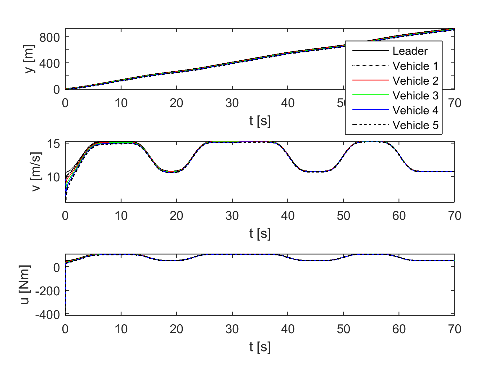
and a gain $\beta=100$ is chosen, which will be greater than $\alpha_{k}$ for all vehicle parameters below. The reference signal for the entire formation is imposed by the control of the leader vehicle, namely $w_{0}(t)$ , which consists of three smoothed rectangular pulses between the levels 15 and 30 Nm. There are six vehicles in total including the leader, and they start at relatively small separations of about $2$ m, with an initial velocity of $10$ m/s.

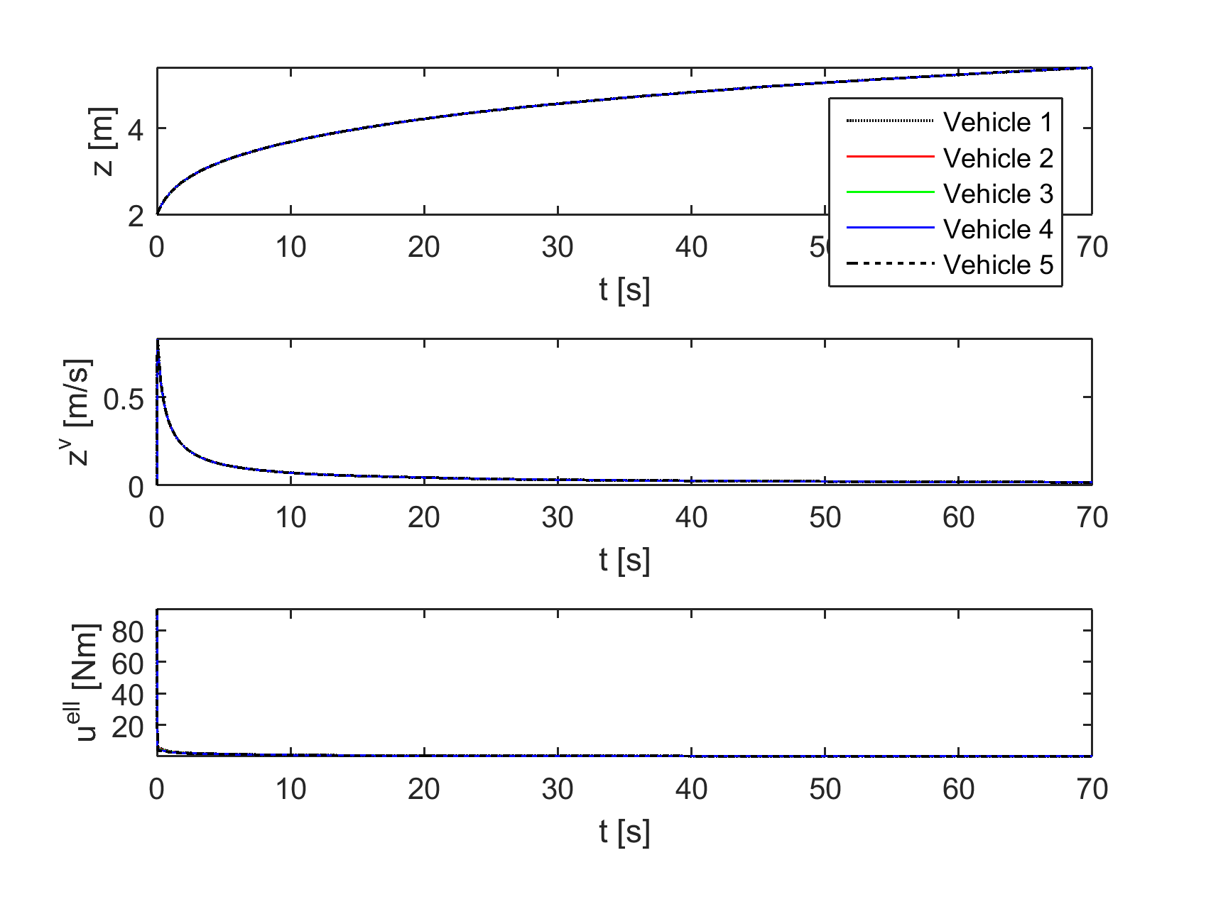
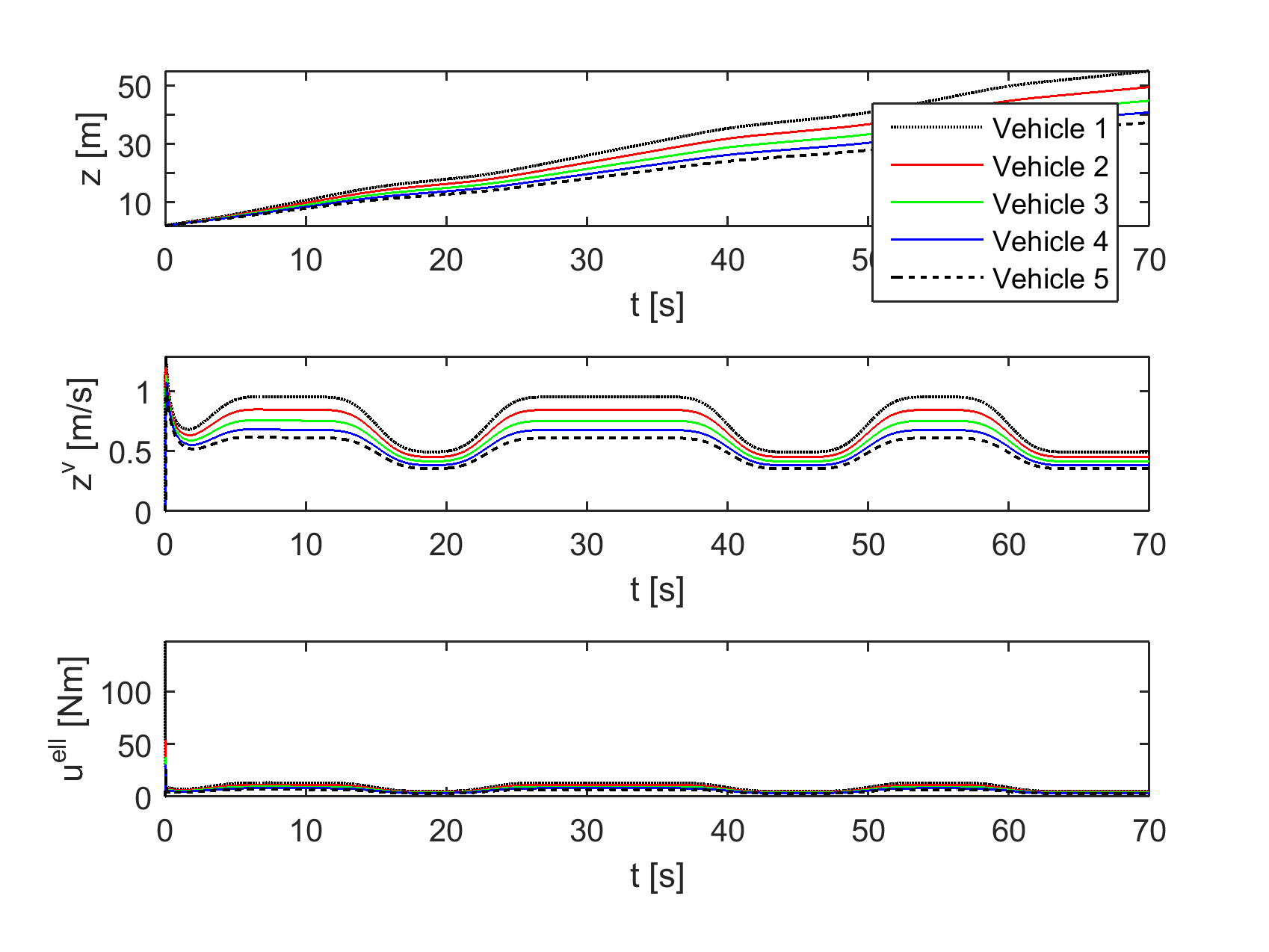
For our baseline experiment, we take homogeneous vehicle dynamics with $\gamma_{k}=0.011$ and $\ell_{k}=0.463$ kg/m for all vehicles $k$ , and no delay. Note that in this case the term $-f_{k}(v_{k})+f_{k-1}(v_{k})$ from (7) disappears. Figure 3, top shows the states and controls of the vehicles using absolute values to give an idea of their true trajectories; in Figure 3, bottom the corresponding interspacing distances $z_{k}$ , velocity differences $z_{k}^{v}$ , and relative controls $u_{k}^{\ell}$ are reported. All subsequent figures will use such relative values. The baseline results show how the controllers initially prioritize increasing interspacing distances, after which the velocities are brought together. Note that on the timeline of this experiment the interspacings have not yet converged; by allowing the experiment to run longer we have confirmed that the steady-state interspacings are 10.95 m, equal to the minimum of the potential function chosen (the trajectories are not shown here since they are not much more informative than Figure 3).

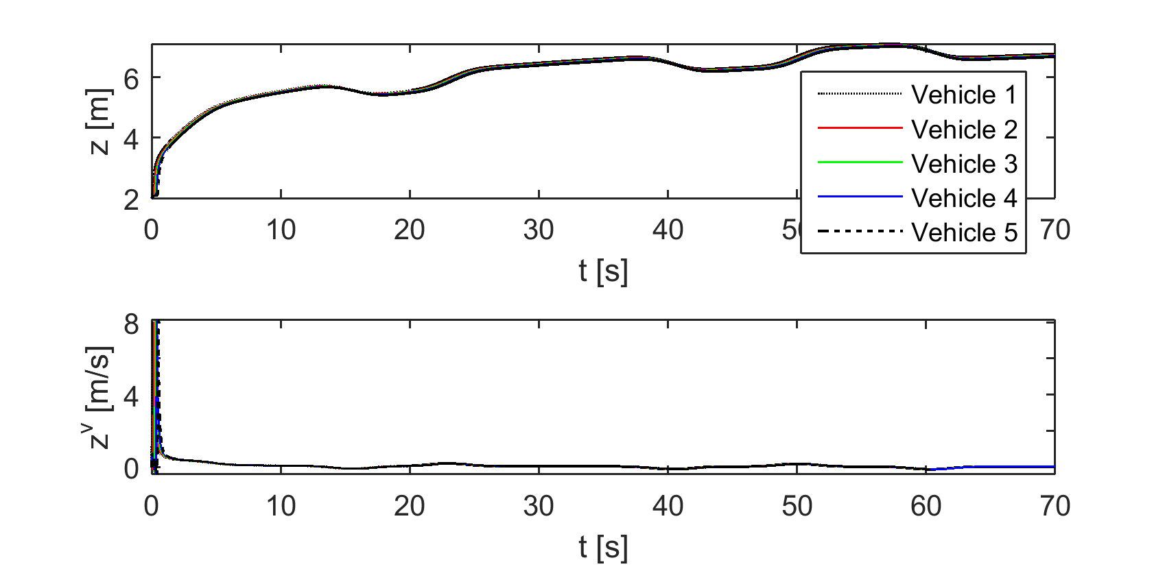
To verify Proposition IV.3, the previous vehicle’s input $u_{k-1}$ is removed from the control law of vehicle $k$ . Figure 4 shows that, indeed, velocity agreement cannot be achieved, leading to divergence of the positions.

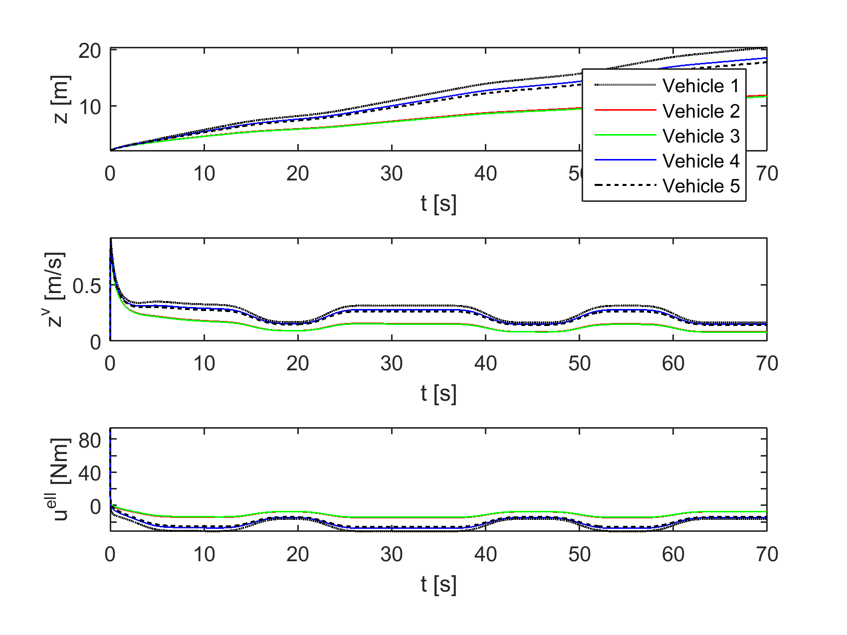
Next, we take heterogeneous vehicle dynamics: in order from the leader $k=0$ to vehicle $k=5$ , $\gamma_{k}=0.003,0.007,0.011,0.015,0.019,0.023$ and $\ell_{k}=0.3,0.4,0.45,0.5,0.6,0.7$ . First we keep the control form of the baseline experiment, without the term $-f_{k}(v_{k})+f_{k-1}(v_{k})$ , to illustrate the need of compensating for vehicle heterogeneity. The results are shown in Figure 5, top, where it is clearly seen that velocity agreement is lost in this case. If we then introduce the appropriate compensation term, the trajectories are those from Figure 5, bottom, with nearly the same performance as in Figure 3. Therefore, the controller efficiently compensates the heterogeneity. Note also the need to apply different control inputs to the vehicles due to their different dynamics.

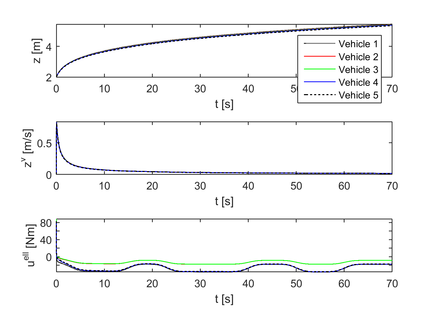
On top of heterogeneity we now introduce a time delay of $\theta=0.2$ s, which is quite conservative (about ten times the actual values) for digital radio communications and we apply the delay compensation mechanism from Section V. The trajectories are those from Figure 6. Note that the quantities reported are the actual instantaneous differences $z_{k}=y_{k-1}(t)-y_{k}(t)$ , $z^{v}_{k}=v_{k-1}(t)-v_{k}(t)$ , and not the actual regulated measurement (31) from Section V.

VI-A A Heuristic for Optimal Control

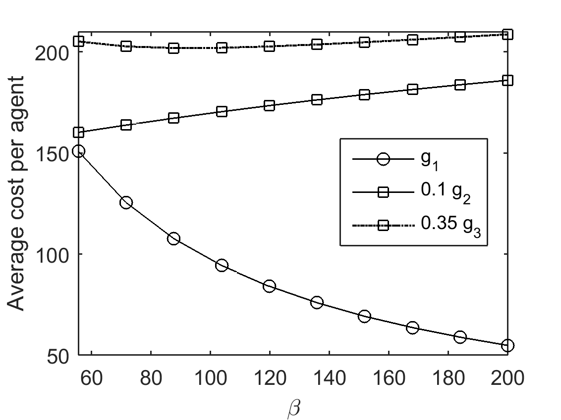
Since the stability analysis holds for any gain $\beta_{k}\geq\alpha_{k}$ , a relevant practical problem is finding a good value for this gain. It turns out that this value depends on the particular objectives of the user. To illustrate, we choose several cost functions and optimize $\beta$ in the baseline experiment, for which $\forall k,\alpha_{k}=55.56=:\alpha$ . Optimization is done by gridding the interval $[\alpha,200]$ into $10$ values, setting all the follower gains to each value of $\beta$ in turn, and experimentally measuring the cost across all follower vehicles, integrated over time and averaged over the followers. The maximum of the range (here, $200$ ), is related to the maximum inputs that the vehicles can apply. The results are shown in Figure 7. The first cost function penalizes velocity disagreements and the control effort: $g_{1}(z,z_{v},u^{\ell})={(z^{v})}^{2}+{(u^{\ell})}^{2}$ (we skip vehicle indices since the cost function is the same for al the vehicles). In this case, larger $\beta$ values are better, so we suggest taking the largest value that is achievable given the physical limits of the vehicles’ drive train. However, if we introduce a “safety” premium and add a ‘barrier’ term $100/{|z|}$ to penalize relatively small interspacing distances, obtaining cost function $g_{2}$ , the situation is reversed: the larger $\beta$ values focus too much on reducing velocity disagreements to the detriment of the interspacing distances, so in this case $\beta=\alpha$ works best. Depending on the particular weights, the optimal value may also be inside the interval, e.g. for $g_{3}(z,z_{v},u^{\ell})=30/{|z|}+{(z^{v})}^{2}+{(u^{\ell})}^{2}$ , $\beta\approx 88$ works best (keeping in mind the resolution of our grid is limited; to find a better approximation of the true optimum, a simple sample-based optimization method could be used, such as golden section rule or even binary search).

VII Conclusions

We have presented a novel method for the distributed control of a string of heterogenous, nonlinear agents guaranteeing collision avoidance and topology preservation in the presence of communication induced time-delays. Numerical experiments seem to suggest that the proposed scheme also benefits from a remarkable robustness to time-varying delays. The study of the root cause of this robustness is the scope of future investigations along with the study of more complicated cost functionals $\mathcal{J}(\cdot)$ , introduced in Subsection IV-B and also the study of more general formation topologies, including those containing self-loops.

References

[1] A. Jadbabaie, J. Lin, and A. Morse, “Coordination of groups of mobile autonomous agents using nearest neighbors rules,” Automatic Control, IEEE Transactions on, vol. 48, no. 6, pp. 988–1001, 2003.
[2] J. Fax and R. Murray, “Information flow and cooperative control of vehicle formations,” IEEE Transactions on Automatic Control, vol. 49, no. 9, pp. 1465–1476, September 2004.
[3] E. Mallada and A. Tan, “Synchronization of weakly coupled oscillators: coupling, delay and topology,” Journal of Physics A: Mathematical and Theoretical, vol. 46, no. 50, p. p. 505101, 2013.
[4] H.Sayyaadi and M. Moarref, “A distributed algorithm for proportional task allocation in networks of monile agents,” IEEE Transactions on Automatic Control, vol. 56, no. 2, pp. 405–410, February 2011.
[5] H.Zhang, Z.Chen, L.Yan, and Y.Wu, “Applications of collective circular motion control to multirobot systems,” IEEE Transactions on Control Syst. Tech, vol. 21, no. 4, pp. 1416–1422, 2013.
[6] R. Olfati-Saber and R. Murray, “Consensus problems in networks of agents with switching topologies and time delays,” IEEE Transactions on Automatic Control, vol. 49, no. 9, pp. 1520–1533, September 2004.
[7] W. Ren and E. Atkins, “Second order consensus protocols in multiple vehicle systems with local interactions,” in AIAA Guidance, Navigation Control Conf. Exhib. San Francisco, CA, USA, 2005.
[8] L. Pecora and T. Caroll, “Synchronization in chaotic systems,” Phys. Rev. Letters, vol. 64, no. 8, p. 821, 1990.
[9] H.Su, X. Wang, and Z. Lin, “Synchronization of coupled harmonic oscillators in a dynamic proximity network,” Automatica, vol. 45, no. 10, pp. 2286–2291, 2009.
[10] N. Chopra and M.Spong, “On exponential synchronization of kuramoto oscillators,” IEEE Transactions on Automatic Control, vol. 54, no. 2, pp. 353–357, February 2009.
[11] L. Pecorra and T. Caroll, “Master stability functions for synchronized coupled systems,” Phys. Rev. Letters, vol. 80, no. 10, p. 2109, 1998.
[12] J. Lu, J. Cao, and D. Ho, “Adaptive stabilization and synchronization for chaotic lur’e systems with time-varying delay,” IEEE Transactions on Circuits Syst. I, vol. 55, no. 5, pp. 1347–1356, May 2008.
[13] L.Scardoci and R. Sepulchre, “Synchronization in networks of identical linear systems,” Automatica, vol. 45, no. 11, pp. 2557–2562, 2009.
[14] l. Zhu, Z. Chen, and R. Middleton, “A general framework for robust output synchronization of heterogenous nonlinear networked systems,” IEEE Transactions on Automatic Control, vol. 61, no. 8, 2016.
[15] H. Kwakernaak and R. Sivan, Linear Optimal Control Systems, J. W. . Sons, Ed. Wiley-Interscience, 1972.
[16] Z. Li, Z. Duan, G. Chen, and L. Huang, “Consensus of multiagent systems and synchronization of complex networks: A unified viewpoint,” IEEE Transactions on Circuits Syst. I, vol. 57, no. 1, pp. 213–224, January 2010.
[17] Z. D. Z. Li and G. Chen, “Dynamic consensus of linear multiagent systems,” ControlTheory Applic. IET, vol. 5, no. 1, pp. 19–28, 2011.
[18] S. Tuna, “Consitions for synchronizability in arrays of coupled linear systems,” IEEE Transactions on Automatic Control, vol. 54, no. 10, pp. 2416–2410, October 2009.
[19] C. Ma and J. Zhang, “Necessary and sufficient conditions for consensuability of linear multiagent systems,” IEEE Transactions on Automatic Control, vol. 55, no. 5, pp. 1263–1268, May 2010.
[20] J. Seo, H. Shim, and J. Back, “Consensus of high order linear systems using dynamic output feedback compensator,” Automatica, vol. 45, no. 11, pp. 2659–2664, 2009.
[21] P.Weiland, R. Sepulchre, and F. Allgower, “An internal model principle is necessary and sufficient for linear output synchronization,” Automatica, vol. 47, no. 5, pp. 1068–1074, 2011.
[22] H. Kim, H. Shim, and J. Seo, “Output consensus of heterogenous uncertain linear multiagent systems,” IEEE Transactions on Automatic Control, vol. 56, no. 1, pp. 200–206, 2011.
[23] H. Grip, A. Saberi, and A. Stoorvogel, “On the existence of virtual exosystems for synchronized linear networks,” Automatica, vol. 49, no. 10, pp. 3145–3148, 2013.
[24] J. Lunze, “Synchronization of heterogenous agents,” IEEE Transactions on Automatic Control, vol. 57, no. 11, pp. 2885–2890, November 2012.
[25] Ş. Sabău, C. Oară, S. Warnick, and A. Jadbabaie, “Optimal distributed control for platooning via sparse coprime factorizations,” IEEE Transactions on Automatic Control, vol. 62, no. 1, pp. 305–320, 2017.
[26] Z. Qu, J. Chunyu, and J. Wang, “Nonlinear cooperative control for consensus of nonlinear and heterogenous systems,” in Proceedings of 46th IEEE Conference on Decision and Control, 2007, pp. 2301–2308.
[27] N. Chopra and M. Spong, Output synchronization of nonlinear systems with relative degree one, ser. Recent Advances in Learning and Control. New York, NY, USA: Springer Verlag, 2008.
[28] W. Yu, G. Chen, and M. Cao, “Consensus in directed networks of agents with nonlinear dynamics,” IEEE Transactions on Automatic Control, vol. 56, no. 6, pp. 1436–1441, June 2011.
[29] H. Su, G. Chen, X. Wang, and Z. Lin, “Adaptive second order consensus of networked mobile agents with nonlinear dynamics,” Automatica, vol. 47, no. 2, pp. 368–375, 2011.
[30] P. W. andF. Allgower, “An internal model principle for synchronization,” in Proc. 7th IEEE Int. Conf. Control Autom, 2009, pp. 285–190.
[31] L. Zhu and Z. Chen, “Robust homogenization and consensus of nonlinear multiagent systems,” Systems & Control Letters, vol. 65, pp. 50–55, 2014.
[32] Z. Chen, “Pattern synchronization of nonlinear heterogenous multiagent networks with jointly connected toplogies,” IEEE Transactions on Networked Systems, vol. 1, no. 4, pp. 349–359, 2014.
[33] Y. Su and J. Huang, “Cooperative global output regulation of heterogenous second-order nonlinear uncertain multiagent systems,” Automatica, vol. 49, no. 11, pp. 2245–3350, 2013.
[34] J. Huang and Y. Su, “Cooperative global robust output regulation for nonlinear uncertain multi-agent systems in lower triangular form,” Automatica, vol. 60, no. 9, pp. 2378–2389, 2015.
[35] A. Isisdori, L. Marconi, and G. Casadei, “Robust output synchronization of a network of heterogenous nonlinear agents via nonlinear regulation theory,” IEEE Transactions on Automatic Control, vol. 59, no. 10, pp. 2680–2691, October 2014.
[36] X. Chen and Z. Chen, “Robust perturbed output regulation and synchronization of nonlinear heterogenous multiagents,” IEEE Tarsn. on Cybernetics.
[37] J.Baillieul and A. Suri, “Information patterns and hedging brockett’s theorem in controlling vehicle formations,” in Decision and Control, 2003. Proceedings. 42nd IEEE Conference on, December 2003, pp. 556–563.
[38] B. Anderson, C. Yu, B. Fidan, and J. Hendrickx, “Rigid graph control architectures for autonomous formations,” IEEE Control Systems Magazine, no. 1, pp. 48–63, December 2008.
[39] S. Mou, A. Morse, M. Belabbas, and B. Anderson, “Undirected rigid formations are problematic,” Preprint on arxiv.org, pp. 1–42, March 2015.
[40] K.-K. O. M.-C. P. H.-S. Ahn, “A survey of multi–agent formation control,” Automatica, vol. 53, pp. 424–440, March 2015.
[41] J. Ploeg, D. Shukla, N. Wouw, and H. Nijmeier, “Controller synthesis for string stability of vehicle platoons,” Intelliogent Transportation Systems, IEEE Transactions on, vol. 15, no. 2, pp. 854–865, 2014.
[42] J. Zhou, X. Wu, W. Yu, M. Small, and J. Lu, “Flocking of multi–agent dynamical systems based on pseudo–leader mechanism,” Systems & Control Letters, vol. 61, pp. 195 – 202, 2012.
[43] Ş. Sabău, I.-C. Morărescu, L. Buşoniu, and A. Jadbabaie, “Decoupled–dynamics distributed control for strings of nonlinear autonomous agents,” in Proceedings of IEEE American Control Conference, 2017.
[44] C. Somarakis and N. Motee, “Nonlinear flocking with fixed distances,” vol. 49-18, IFAC - Papers Online. Elsevier Ltd., 2016, pp. 576–581.
[45] F. Cucker and S. Smale, “Emergent behavior in flocks,” IEEE Transactions on Automatic Control, vol. 52, no. 5, pp. 852–862, 2007.
[46] F. Cucker and J. Dong, “A general collision-avoiding flocking framework,” IEEE Transactions on Automatic Control, vol. 56, no. 5, pp. 1124–1129, 2011.
[47] A. P. R. M. O. Mason, “Leader tracking in homogeneous vehicle platoons with broadcast delays,” Automatica, vol. 50, pp. 64–75, 2014.
[48] A. Peters, R. Middleton, and O. Mason, “Leader tracking in homogeneous vehicle platoons with broadcast delays,” Automatica, vol. 50, pp. 64–74, 2014.
[49] J. I. Ge and G. Orosz, “Optimal control of connected vehicle systems with communicatio delay and driver reaction time,” IEEE Trans. Intelligent Transp. Systems, vol. 18, no. 8, pp. 2056–2070, August 2017.
[50] L. Zhang and G. Orosz, “Consensus and disturbance attenuation in multi-agent chains with nonlinear control and time delays,” Int. Journal of Robust and Nonlinear Control, vol. 27, pp. 781–803, August 2017.
[51] C. Chien and P. Ioannou, “Automatic vehicle following,” in Proceedings of IEEE American Control Conference, 1992, pp. 1748–1752.
[52] S. Klinge and R. Middleton, “Time headway requirements for string stability of homogeneous linear unidirectionally connected systems,” in Proceedings of 48th IEEE Conference on Decision and Control, 2009, pp. 1992–1997.
[53] D. Swaroop, J. Hedrick, C. Chien, and P. Ioannou, “A comparison of spacing and headway control laws for automatically controlled vehicles,” Vehicle System Dynamics, vol. 23, no. 1, pp. 597 – 625, 1994.
[54] R. H. Middleton and J. Braslavsky, “String stability in classes of linear time invariant formation control with limited communication range,” IEEE Transactions on Automatic Control, vol. 55, no. 7, pp. 1519–1530, 2010.
[55] G. Orosz and S. Shah, “A nonlinear framework for autonomous cruise control,” in ASME 5–th Annual Dynamic Systems and Control Conference joint with JSME 11–th Motion and Vibration Conference, 2012.

Dynamics–Decoupling Control for Strings of Heterogenous Nonlinear Autonomous Agents

Abstract

I Introduction

I-A Motivation and Scope of Work

I-B Contributions of the Paper

I-C Paper Organization

II General Framework and Problem Statement

Definition II.1

Definition II.2

Definition II.3

II-A Distributed Trajectory Tracking in the String Formation

Assumption II.4

III A Practical Distributed Control Architecture

Remark III.1

Remark III.2

III-A A First Glance at the Closed–Loop Dynamics Decoupling

Lemma III.3

Proof:

IV Decoupling control design

Theorem IV.1

Proof:

Remark IV.2

IV-A Communicating the Control Signals of the sub-Controllers

Proposition IV.3

Proof:

IV-B Some Considerations and Future Work

IV-C Platooning Control

V A Practical Time-Delays Compensation Mechanism

V-A Adapting Time-Headways for Delays Compensation

Remark V.1

Remark V.2

V-B Changing the Regulated Measurements

Proposition V.3

Proof:

Remark V.4

Remark V.5

V-C A Controller to Cope with Time Delays

Remark V.6

Theorem V.7

Proof:

Remark V.8

VI A Numerical Example and Further Considerations

VI-A A Heuristic for Optimal Control

VII Conclusions

References

Dynamics–Decoupling Control for Strings
of Heterogenous Nonlinear Autonomous Agents