Earthquake Magnitude and b value prediction model using Extreme Learning Machine

Gunbir Singh Baveja
University of British Columbia
Vancouver, BC V6T 1Z4
gbaveja@student.ubc.ca
&

Jaspreet Singh
Department of Computer Science and Engineering
GD Goenka University
Sohna Rural, India
jaspreet.singh@ggdu.org
Research was not conducted under the affiliation of University of British Columbia, Vancouver.

(November 30, 2021)

Abstract

Earthquake Prediction has been a challenging research area for many decades, where the future occurrence of this highly uncertain calamity is predicted. In this paper, several parametric and non-parametric features were calculated, where the non-parametric features were calculated using the parametric features. 8 seismic features were calculated using Gutenberg-Richter law, total recurrence time, seismic energy release. Additionally, criterions such as Maximum Relevance and Maximum Redundancy were applied to choose the pertinent features. These features along with others were used as input for an Extreme Learning Machine (ELM) Regression Model. Magnitude and Time data of 5 decades from the Assam-Guwahati region were used to create this model for magnitude prediction. The Testing Accuracy and Testing Speed were computed taking Root Mean Squared Error (RMSE) as the parameter for evaluating the model. As confirmed by the results, ELM shows better scalability with much faster Training and Testing Speed (up to thousand times faster) than traditional Support Vector Machines. The Testing RMSE (Root Mean Squared Error) came out to be. To further test the model’s robustness, magnitude-time data from California was used to- calculate the seismic indicators, fed into neural network (ELM) and tested on the Assam-Guwahati region. The model proves to be successful and can be implemented in early warning systems as it continues to be a major part of Disaster Response and Management.

Keywords Earthquake Prediction $\cdot$ Machine Learning $\cdot$ Extreme Learning Machine $\cdot$ Seismological Features

1 Introduction

Earthquake is one of the most destructive and the deadliest natural disaster that has caused thousands of deaths, and millions if not billions of dollars in property loss. No part of the world is immune to earthquakes. The developing countries, in particular, are the most affected because emergency response services may not be available even in stressful times. A reliable early warning system may potentially be able to save lives and land. Since the biggest and deadly earthquakes started occurring near the 1950s, primitive prediction methods were thought as necessities. But by the 1990s, continuing failure led to many questions whether it was even possible to foretell the Time-Location of Earthquakes.

Refer to caption — Figure 1: All the earthquakes ( $1653$ ) in the north-eastern region of India (Assam-Guwahati) between $1933-2020$ .

Fortunately, with the emergence of modern computer science based intelligent algorithms, it is relatively easy to predict or classify data which has a definite pattern. Significant results have been attained in different fields of study such as Flood Forecasting (Anupam and Pani, 2019), Weather Analysis and Forecasting (Mishra et al., 2013), and disease diagnosis (Cosma et al., 2016). Machine Learning and seismology can be linked together to produce considerable results.

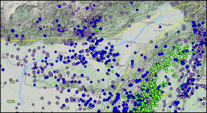
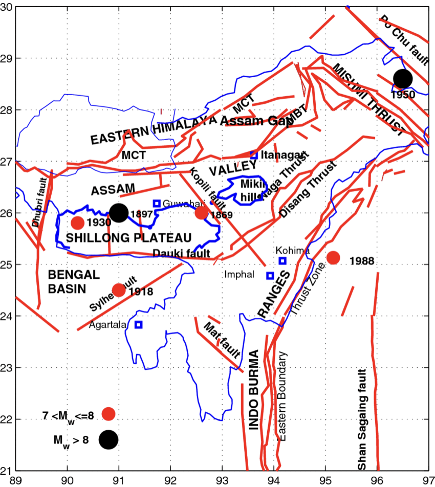
Assam-Guwahati region is the most earthquake prone region of India due to subducting Indian plate under the Eurasian plate. This region has been experiencing earthquakes of significant magnitude at moderate depth. A polygon shaped Assam region was selected for calculation of seismic features. Machine Learning and Computational Intelligence has led to paradigm shift in the methods of predictions and determination of earthquakes. An ideal earthquake predictor must yield the Magnitude, Time, Energy release and Location of the earthquake. Although our prediction model isn’t perfect, it is indeed a huge step forward in Earthquake research.

The core idea of this work is to predict earthquakes with magnitude $4.5+$ and also predict the number of days in between successive earthquakes. The mathematically calculated seismic features were used as an input to the SLFN (Single Layer Feed-Forward Network). The prediction results of the neural network and SVM were compared and discussed in this paper.

1.1 Tectonics of Assam region

Assam is one of the most seismically active regions in India with events occurring at shallow depth (0-70km). The region was geologically formed due to collision of Eurasian and Indian Plate during Eocene. The seismic parameters are mathematically calculated from a catalogue, so the catalogue should be complete above the cut- off magnitude. Here, the cut-off magnitude refers to the earthquake magnitude, below which seismic events are not considered for parameter calculations ( $4.0$ in our case). See Section 3.

2 Literature Review

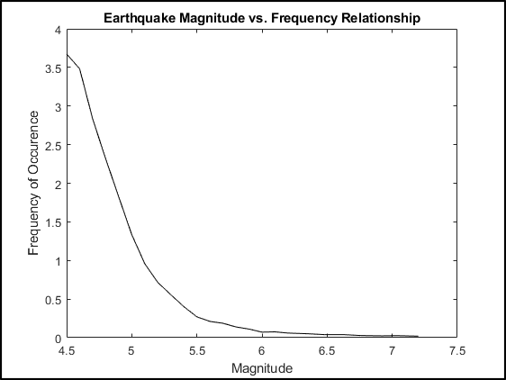
Various studies have been carried out by researchers over earthquake occurrences and predictions leading to various conclusions. The Gutenberg-Richter mathematical model is one such example where the relationship between earthquake magnitude and frequency was calculated; the relationship is analysed and used to predict distribution over time. (Petersen et al., 2019) carried out research under the umbrella of California Geological Survey (CGS) and proposed a time-independent model showing that probability of earthquake occurrence follows poisson’s distribution model.

Several approaches have been proposed in the literature for using artificial neural networks (ANNs) to predict earthquakes based on various seismic precursors. For example, (Negarestani et al., 2002) used a backpropagation neural network (BPNN) to identify abnormal changes in soil radon concentration, which can be induced by earthquakes, by differentiating them from normal environmental variations. (Liu et al., 2004) employed an ensemble of radial basis function (RBF) neural networks to forecast earthquakes in China using historical magnitude data as input. (Hossain et al., 2018) presented an expert system-based method for earthquake prediction that involves dividing the globe into four quadrants, using historic earthquake data as input and applying predicate logic and association rules to make predictions for each quadrant over a 24-hour period.

In their paper, (Asim et al., 2017) used four machine learning techniques, including a pattern recognition neural network, a recurrent neural network, a random forest, and a linear programming boost ensemble classifier, to predict earthquake magnitudes in the Hindukush region using a temporal sequence of past seismic activity. Earthquake precursors are phenomena that occur before a main shock and are causally linked to it, rather than simply occurring before it in time (Habermann, 1988). These precursors can be based on continuous observations of various physical parameters such as seismic wave velocity, gravity, resistivity, and electricity (Nuannin, 2006). For example, (Lu et al., 2002) found that drops in underground water levels and changes in resistivity recorded by geoelectric stations within $180$ km of the epicenter preceded the $M=7.8$ Tangshan earthquake.

Other proposed precursors include changes in seismicity rates, source parameters of earthquakes, and frequency-magnitude distributions (FMD) ((Nuannin, 2006); (Enescu and Ito, 2003); (Nagao et al., 2002); (Monterroso and Kulhánek, 2003); (Nuannin, 2006); (Schorlemmer et al., 2003); (Schorlemmer et al., 2005); (Wyss and Habermann, 1979); (Wyss and Martirosyan, 1998)). Seismic quiescence, or periods of significantly reduced seismicity, has also been suggested as a potential precursor (Katsumata and Kasahara, 1999).

3 Seismic Parameters

This study is carried out by using the eight seismic indicators, which are basically meant to represent the seismic state and potential of the ground. This section contains the overview of all the parameters and their calculation. One of the parameters is the Time T, which is the time span over the last n number of events and n in our case is 100 and t represents the time of earthquake occurrence.

T=t_{n}-t_{1}

(1)

3.1 Mean Magnitude

Time T represents the frequency of foreshocks before the month under consideration. The second seismic indicator considered is the mean magnitude of the last n events. It relates to the magnitudes of foreshocks, since the magnitude M of seismic activity increases before a larger earthquake.

M_{\text{mean}}=\frac{\sum_{i}M}{n}.

(2)

3.2 Seismic Energy

The rate of square root of seismic energy release dE is another seismic indicator that can be related to seismic activity through the phenomenon of seismic quiescence. Seismic energy releases gradually from fault lines through low-magnitude seismic events but if this phenomenon gets disturbed, it may lead to a major seismic event. The equation for square root of seismic energy released is given below:

\mathrm{d}E^{\frac{1}{2}}=\frac{\sum\left(10^{10.8+1.5M}\right)^{\frac{1}{2}}}{T}

(3)

3.3 $a$ and $b$ value

The Frequency-Magnitude Distribution describes the number of earthquakes occurring in a given region as a function of their magnitude M as:

\log N_{i}=a-bM_{i},

(4)

where $N$ is the cumulative number of earthquakes with magnitude equal to or larger than $M$ , and $a$ and $b$ are real constants that may vary in space and time.

The parameter $a$ characterizes the general level of seismicity in a given area during the study period, i.e., the higher the $a$ value, the higher the seismicity (Nuannin, 2006). The parameter $b$ is believed to depend on the stress regime and tectonic character of the region (Bhatt et al., 2009).

The $a$ and $b$ values are calculated numerically through two different methods. In earthquake prediction study for North-Eastern India, linear least square regression analysis based method is proposed.

$\displaystyle b_{\text{lsq}}$	$\displaystyle=\frac{\left(n\sum M_{i}\log N_{i}-\sum M_{i}\sum\log N_{i}\right)}{\left(\sum M_{i}\right)^{2}-n\sum M_{i}^{2}}$	(5)
$\displaystyle b_{\text{mlk}}$	$\displaystyle=\frac{\log_{10}e}{\text{mean}(M)-\min(M)}$	(6)
$\displaystyle a_{\text{lsq}}$	$\displaystyle=\sum\frac{\left(\log_{10}N_{i}+b_{\text{lsq}}M_{i}\right)}{n}$	(7)
$\displaystyle a_{\text{mlk}}$	$\displaystyle=\log_{10}N+b_{\text{mlk}}\cdot\min(M).$	(8)

5 and 7 represent the linear least square regression while 6 and 8 show the maximum likelihood method for calculation of $a$ and $b$ values.

Figure 4: The following graph shows

a

and

b

values calculated from the Assam-Guwahati region Earthquake data. The

b

value tends to be closer to

0.85

indicating moderate-high number of small scale earthquakes. Total Mean Deviation of

b

value is

~0.368

Figure 5: The following graph shows

a

and

b

values calculated from the California Earthquake data. The

b

value is closer to

1

indicating a seismically active region

In earthquake prediction study for North-Eastern India, linear least square regression analysis based method is proposed along with real time calculation of $a$ and $b$ values in this study.

3.4 Deviation from Gutenberg-Richter Law

Deviation of actual data from Gutenberg-Richter inverse power law (4) is also considered as a seismic indicator (Serra and Corral, 2017). We calculate it using the general variance model, where a greater $a-bM_{i}$ value corresponds to a greater conformance and therefore– more likely to be predicted by the inverse power law:

\sigma=\frac{\sum\left(\log N-a-bM\right)^{2}}{n-1}.

(9)

Figure 6: The graph shows the deviation from Gutenberg-richter law for the Assam-Guwahati region

Figure 7: The graph shows the deviation from Gutenberg-richter law for the California region

3.5 Expected Magnitude

The difference between the maximum observed and the maximum occurred earthquake magnitude is also considered as a seismic indicator (refer to figure 9 and 9). The maximum observed event is listed in the catalog, while maximum expected event is obtained using the equation

M_{\text{expected}}=\frac{a}{b},

(10)

where $a$ is the $y$ -intercept in the inverse power law obtained from 4.

Figure 8: Expected Magnitude of the Assam-Guwahati region calculated as per the respective

a

and

b

values

Figure 9: Expected Magnitude of the California region calculated as per the respective

a

and

b

values

3.6 Maximum magnitude in last seven days

The maximum magnitude recorded in the days previous to $E_{t}$ is also considered as an important seismic parameter ((Wang, 2015); (Alarifi et al., 2012)) and is represented as

x_{6i}=\max(M_{i}),\text{where }t\in[-7,0).

(11)

3.7 Total recurrence time

It is also known as probabilistic recurrence time ( $T_{r}$ ) and is defined as the time between two earthquakes of magnitude greater than or equal to $M^{\prime}$ and is calculated using 12. This parameter is another interpretation of Gutenberg-Richter’s law. As evident from the statement of inverse law, there will be different value of $T_{r}$ for every different value of $M^{\prime}$ , which would increase with increasing magnitude.

T_{r}=\frac{T}{10^{a-bM^{\prime}}}.

(12)

Available literature does not focus on which value of $M^{\prime}$ to be selected in such a scenario therefore $T_{r}$ is calculated for every $M^{\prime}$ from $4.0$ to $6.0$ magnitudes following the principle of retaining maximum available information. So for two sets of $a$ and $b$ values along with varying $M^{\prime}$ adds $42$ seismic features to the dataset.

3.8 Probability of earthquake occurrence

The probability of earthquake occurrence of magnitude greater than or equal to $6.0$ is also taken as an important seismic feature. It is represented by $x_{7i}$ and calculated through 13. The inclusion of this feature supports the inclusion of Gutenberg-Richter law in an indirect way. The value of $x_{7i}$ is dependent upon the corresponding $b$ value:

x_{7i}=e^{\frac{-3b_{i}}{\log e}}.

(13)

Therefore, $b_{\text{lsq}}$ and $b_{\text{mlk}}$ are separately used to calculate $x_{7}i$ , thus giving two different values for this seismic feature.

4 Earthquake Magnitude Prediction model

Unlike previous other earthquake magnitude prediction models proposed, in this paper a new learning algorithm was used which consists of Single Layer Feed-forward Neural network (SLFN). This algorithm along with minimum Redundancy Maximum Relevance (mRMR) added to the hardiness of the model. The layout of the final prediction is given below. The dataset of the region was divided into Training and Testing sets. $75\%$ of the data for training and testing was performed on the rest $25\%$ of the data. All the parameters were taken into consideration while training and their variance within time.

Figure 10: Flow Chart of the ELM Model used to predict earthquake magnitude in Assam and California

The proposed procedure includes the two step feature selection. The features are selected after performing relevancy and redundancy checks, to make sure that only useful features are employed for earthquake prediction. The selected set of features was then passed on to Extreme Learning Machine (ELM).

4.1 Extreme Learning Machine (ELM)

ELM consists of a Single Layer Feed-Forward Neural Network where the parameters of the hidden nodes may not be tuned(Ding et al., 2015). This is an excellent feature which avoids the use of other Optimization Algorithms like Particle Swarm Optimization (PSO)(Kennedy and Eberhart, 1995), Salp Swarm Optimization (SSA)(Mirjalili et al., 2017). Here is a brief explanation of ELM (Nagao et al., 2002).

Given $N$ distinct training samples $(\mathcal{X}_{i},\mathfrak{t}_{i})$ , where $\mathcal{X}_{i}=[x_{i1},x_{i2},\ldots,x_{in}]^{T}\in\mathbb{R}^{n}$ and $\mathfrak{t}_{i}=[t_{i1},t_{i2},\ldots,t_{in}]^{T}\in\mathbb{R}^{m}$ , the output of a SLFN with $Y$ hidden nodes (additive or RBF nodes) can be represented by:

o_{j}=\sum\limits_{i=1}^{Y}\beta_{i}f_{i}(\mathcal{X}_{j})=\sum\limits_{i=1}^{Y}\beta_{i}g_{i}\left(\mathcal{W}_{i}\cdot\mathcal{X}_{j}+b_{i}\right),\hskip 72.26999pt\text{for $j\in[1,N]$}.

(14)

where $\mathcal{W}_{i}=[w_{i1},w_{i2},\ldots,w_{in}]^{T}$ represents the weight vector that connects the hidden node and $j$ th output. $\beta_{i}=[\beta_{i1},\beta_{i2}.\ldots,\beta_{im}]^{T}$ represents the weight vector that connects the hidden node and the $i$ th output nodes.

$o_{j}$ is the output vector of the SLFN with respect to the input sample $x_{i}$ . $a_{i}=\left[a_{i1},a_{i2},\ldots,a_{in}\right]^{T}$ and $b_{i}$ are learning parameters generated randomly of the $j$ th hidden node, respectively.

The standard of SLFNs and L hidden nodes in the activation function $g(x)$ can be taken as samples of N without error. In other words,

\sum\limits_{i=1}^{Y}\beta_{i}g_{i}\left(\mathcal{W}_{i}\cdot\mathcal{X}_{j}+b_{i}\right)=t_{j},\hskip 72.26999pt\text{for $j\in[1,N]$}.

(15)

From the equations given for $N$ , it can then be presented as

H\beta=T

(16)

where

H=\begin{bmatrix}f(a_{1}x_{1}+b_{1})&\cdots&f(a_{Y}x_{1}+b_{Y})\\ \vdots&\ddots&\vdots\\ f(a_{1}x_{N}+b_{1})&\cdots&f(a_{Y}x_{Y}+b_{Y})\\ \end{bmatrix}_{N\times N},\beta=\begin{bmatrix}\beta_{1}^{T}\\ \vdots\\ \beta_{Y}^{T}\end{bmatrix}_{Y\times m},T=\begin{bmatrix}t_{1}^{T}\\ \vdots\\ t_{N}^{T}\end{bmatrix}_{Y\times m}.

(17)

To minimise the cost function $\lVert O-T\rVert$ , ELM theories claim that the hidden nodes’ learning parameters $a$ and $b$ can be assigned randomly without considering the input data. Then, 16 becomes a linear system and the output weights $\beta$ can be analytically determined by finding a least-square solution as follows,

\beta-H^{\dagger}T

(18)

Where $H^{\dagger}$ represents the Moore-Penrose generalized inverse of $H$ . Hence, by mathematical transformation the output weights are calculated. This avoids the lengthy training phase where adjustment of the parameters takes place iteratively along with some learning parameters (such as learning rate and iterations).

Figure 11: A diagram showing the basic ELM Neural Network structure, with the input layer, a hidden layer and an output layer

(Huang et al., 2006) listed the variables, where $H$ represents the output matrix of the hidden layer of the neural network. In $H$ , the $i$ th column is used to describe the $i$ th hidden layer nodes in terms of the input nodes. If $L\leq N$ represents the desired number of hidden nodes, the activation function g becomes infinitely differentiable.

5 Results

The data in this study came from United States Geological Survey. The model was run on a Lenovo G-80 laptop with Intel® Core™ i $5-5200$ U CPU @ $2.20$ GHz and $8.00$ GB RAM. The results can be concluded into the following table: The ELM Model got an RMSE of $~0.08$ which indicates over-fitting in the model. The average relative error percentage in other papers came out to be around 3%. The SVR had an RMSE of $0.043$ with a heavy training time of $2289$ seconds. A significant drop in the testing time is observed in the ELM.

Using this model along with the CTS-M (Continuous Time Serious Markov) model which makes it possible to predict the location region of the next earthquake. This can improve the efficiency of the Early Warning Systems by a mile and also improve time efficacy of disaster response teams. As ELM proved to be better than SVR, it was used to predict earthquake magnitude trained on California Earthquake Data and tested on the Assam-Guwahati Region.

Figure 12: following graph contains the scaled magnitude values predicted by the ELM Neural Network trained over Assam Region vs scaled actual magnitude values

(a) Overall RMSE

(b) Parametric error (cumulative testing error)

Figure 13: RMSE and parametric error of all parameters for ELM trained and tested on the Assam-Guwahati region Data

All models were tested on the Assam-Guwahati region with ratio of $3:1$ with the training data. for the California dataset, it had $26192$ data points and was tested on $8639$ data points.

6 Conclusion

Two Machine Learning techniques have been used to predict earthquakes in the subducting Assam-Guwahati Region, one of the most seismically active regions in India. Both Magnitude Predictors shows significant results when compared to one another.

Further, the better Machine Learning Model (Extreme Learning Machine) was trained on California Dataset and tested on the same Assam-Guwahati Data. This can be improved by using an M-ELM model which reduces the chances of over-fitting. In the end, it can drastically improve the retro-traditional machine learning models. The parameter $b$ (commonly referred to as the " $b$ -value") is commonly close to 1.0 in seismically active regions. This means that for a given frequency of magnitude $4.0$ or larger events there will be $10$ times as many magnitude $3.0$ or larger quakes and $100$ times as many magnitude $2.0$ or larger quakes. There is some variation of $b$ -values in the approximate range of $0.5$ to $2$ depending on the source environment of the region. In a notable portion of the data, the $b$ value seems to less than $1$ and gradually decreases.

The study used real time $b$ value change across time ( $b(t)$ ), change recorded after every earthquake occurrence, instead of taking the $b$ value to be constant throughout one year time. The study shows, although earthquake occurrence is supposed to be decidedly nonlinear and appears to be a random phenomenon, yet it can be modeled on the basis of geophysical facts of the seismic region along with highly sophisticated modeling and learning approaches of machine learning.

Table 1: Result of Earthquake models on the Assam-Guwahati region

	Assam-ELM	SVR	Cali-ELM
Testing Time	$0.109375$ s	$198$ s	$0.5$ s
RMSE	$0.0081675$	$0.043$	$0.4572$
Training Time	$3.140625$ s	$2289$ s	$4$ s

Table 2: Minimum/Maximum and mean

a

and

b

values calculated on the Assam-Guwahati data

Min $b$ -value	Max $b$ -value	Mean $b$ -value
$0.17019$	$0.8533$	$0.3685$

Min $a$ -value	Max $a$ -value	Mean $a$ -value
$0.9988$	$6.6923$	$5.6804$

•

ELM model- trained and tested on Assam region proves to be better.
•

A Significant Drop ( $99.95\%$ in $T_{e}$ , ) in the Testing and Training Time can be observed in the California (ELM) and Assam (ELM) models $(T_{e}<1s,T_{r}<5s).$
•

There exists a trade-off between $T_{e}$ and RMSE of ELM in Assam Data and California, indicating that the model is more sensitive to training data samples.

A smaller $b-$ value likely suggests that the stress is high in the examined region. Decreasing $b$ value within the seismogenic volume under consideration has been found to correlate with increasing effective stress levels prior to major shocks.

Normal faulting is associated with the highest $b-$ values, strike-slip events show mean values and thrust events the lowest values. This observation means that $b$ acts as a stress meter, depending inversely on the differential stress.

References

Anupam and Pani [2019] Sagnik Anupam and Padmini Pani. Flood forecasting using a hybrid extreme learning machine-particle swarm optimization algorithm (ELM-PSO) model. Modeling Earth Systems and Environment, 6(1):341–347, November 2019. doi:10.1007/s40808-019-00682-z. URL https://doi.org/10.1007/s40808-019-00682-z.
Mishra et al. [2013] Ashok Mishra, Christian Siderius, Kenny Aberson, Martine van der Ploeg, and Jochen Froebrich. Short-term rainfall forecasts as a soft adaptation to climate change in irrigation management in north-east india. Agricultural Water Management, 127:97–106, September 2013. doi:10.1016/j.agwat.2013.06.001. URL https://doi.org/10.1016/j.agwat.2013.06.001.
Cosma et al. [2016] Georgina Cosma, David Brown, Matthew Archer, Masood Khan, and Alan Pockley. A survey on computational intelligence approaches for predictive modeling in prostate cancer. Expert Systems with Applications, 70, 11 2016. doi:10.1016/j.eswa.2016.11.006.
Petersen et al. [2019] Mark Petersen, Allison Shumway, Peter Powers, Charles Mueller, Morgan Moschetti, Arthur Frankel, Sanaz Rezaeian, Daniel Mcnamara, Nico Luco, Oliver Boyd, Kenneth Rukstales, Kishor Jaiswal, Eric Thompson, Susan Hoover, Brandon Clayton, Edward Field, and Yuehua Zeng. The 2018 update of the us national seismic hazard model: Overview of model and implications. Earthquake Spectra, 36:875529301987819, 11 2019. doi:10.1177/8755293019878199.
Negarestani et al. [2002] Ali Negarestani, Saeed Setayeshi, M Ghannadi-Maragheh, and B Akashe. Layered neural networks based analysis of radon concentration and environmental parameters in earthquake prediction. Journal of environmental radioactivity, 62:225–33, 02 2002. doi:10.1016/S0265-931X(01)00165-5.
Liu et al. [2004] yu Liu, Qin Zheng, Zhewen Shi, and Junying Chen. Training radial basis function networks with particle swarms. In Advances in Neural Networks, volume 3173, pages 317–322, 08 2004. ISBN 978-3-540-22841-7. doi:10.1007/978-3-540-28647-9_54.
Hossain et al. [2018] Mohammad Hossain, Abdullah Hasan, Sunanda Guha, and Karl Andersson. A belief rule based expert system to predict earthquake under uncertainty. Journal of Seismology, 9, 07 2018. doi:10.22667/JOWUA.2018.06.30.026.
Asim et al. [2017] Khawaja Asim, Francisco Martínez-Álvarez, Abdul Basit, and Talat Iqbal. Earthquake magnitude prediction in hindukush region using machine learning techniques. Natural Hazards, 85:471–486, 01 2017. doi:10.1007/s11069-016-2579-3.
Habermann [1988] R. E. Habermann. Precursory seismic quiescence: Past, present, and future. pure and applied geophysics, 126(2):279–318, 1988. doi:10.1007/BF00879000. URL https://doi.org/10.1007/BF00879000.
Nuannin [2006] Paiboon Nuannin. The potential of b-value variations as earthquake precursors for small and large events. In Journal of Geology, 05 2006.
Lu et al. [2002] Chia-Yu Lu, Hao-tsu Chu, Jian-Cheng Lee, YU-CHANG CHAN, KUO-JIAN CHANG, and Frederic Mouthereau. The 1999 chi-chi taiwan earthquake and basement impact thrust kinematics. Open House, 01 2002.
Enescu and Ito [2003] Bogdan Enescu and Kiyoshi Ito. Values of b and p: their variations and relation to physical processes for earthquakes in japan. Ann. Disas. Prev. Res. Inst. Kyoto Univ., 46B, 01 2003.
Nagao et al. [2002] T. Nagao, Y. Enomoto, Y. Fujinawa, M. Hata, M. Hayakawa, Q. Huang, J. Izutsu, Y. Kushida, K. Maeda, K. Oike, S. Uyeda, and T. Yoshino. Electromagnetic anomalies associated with 1995 kobe earthquake. Journal of Geodynamics, 33(4):401–411, 2002. ISSN 0264-3707. doi:https://doi.org/10.1016/S0264-3707(02)00004-2. URL https://www.sciencedirect.com/science/article/pii/S0264370702000042.
Monterroso and Kulhánek [2003] David A. Monterroso and Ota Kulhánek. Spatial variations of b-values in the subduction zone of central america. Geofisica Internacional, 42:575–587, 2003.
Schorlemmer et al. [2003] D. Schorlemmer, G. Neri, S. Wiemer, and A. Mostaccio. Stability and significance tests for b-value anomalies: Example from the tyrrhenian sea. Geophysical Research Letters, 30(16), 2003. doi:https://doi.org/10.1029/2003GL017335. URL https://agupubs.onlinelibrary.wiley.com/doi/abs/10.1029/2003GL017335.
Schorlemmer et al. [2005] Danijel Schorlemmer, Stefan Wiemer, and Max Wyss. Variations in earthquake-size distribution across different stress regimes. Nature, 437:539–42, 10 2005. doi:10.1038/nature04094.
Wyss and Habermann [1979] M. Wyss and R. E. Habermann. Seismic quiescence precursory to a past and a future kurile island earthquake. pure and applied geophysics, 117(6):1195–1211, 1979. doi:10.1007/BF00876215. URL https://doi.org/10.1007/BF00876215.
Wyss and Martirosyan [1998] Max Wyss and Artak H. Martirosyan. Seismic quiescence before the m7, 1988, spitak earthquake, armenia. Geophysical Journal International, 134(2):329–340, 1998. doi:https://doi.org/10.1046/j.1365-246x.1998.00543.x. URL https://onlinelibrary.wiley.com/doi/abs/10.1046/j.1365-246x.1998.00543.x.
Katsumata and Kasahara [1999] K. Katsumata and M. Kasahara. Precursory seismic quiescence before the 1994 kurile earthquake (mw = 8.3) revealed by three independent seismic catalogs. pure and applied geophysics, 155(2):443–470, 1999. doi:10.1007/s000240050274. URL https://doi.org/10.1007/s000240050274.
Bhatt et al. [2009] Kaushalendra Mangal Bhatt, Andreas Hördt, and Santosh Kumar. Seismicity analysis of the kachchh aftershock zone and tectonic implication for 26 jan 2001 bhuj earthquake. Tectonophysics, 465(1):75–83, 2009. ISSN 0040-1951. doi:https://doi.org/10.1016/j.tecto.2008.11.011. URL https://www.sciencedirect.com/science/article/pii/S004019510800574X.
Serra and Corral [2017] Isabel Serra and Álvaro Corral. Deviation from power law of the global seismic moment distribution. Scientific Reports, 7(1), January 2017. doi:10.1038/srep40045. URL https://doi.org/10.1038/srep40045.
Wang [2015] Zhenming Wang. Predicting or forecasting earthquakes and the resulting ground-motion hazards: A dilemma for earth scientists. Seismological Research Letters, 86:1–5, 01 2015. doi:10.1785/0220140211.
Alarifi et al. [2012] Abdulrahman S.N. Alarifi, Nassir S.N. Alarifi, and Saad Al-Humidan. Earthquakes magnitude predication using artificial neural network in northern red sea area. Journal of King Saud University - Science, 24(4):301–313, October 2012. doi:10.1016/j.jksus.2011.05.002. URL https://doi.org/10.1016/j.jksus.2011.05.002.
Ding et al. [2015] Shifei Ding, Han Zhao, Yanan Zhang, Xinzheng Xu, and Ru Nie. Extreme learning machine: Algorithm, theory and applications. Artif. Intell. Rev., 44(1):103–115, jun 2015. ISSN 0269-2821. doi:10.1007/s10462-013-9405-z. URL https://doi.org/10.1007/s10462-013-9405-z.
Kennedy and Eberhart [1995] J. Kennedy and R. Eberhart. Particle swarm optimization. In Proceedings of ICNN'95 - International Conference on Neural Networks. IEEE, 1995. doi:10.1109/icnn.1995.488968. URL https://doi.org/10.1109/icnn.1995.488968.
Mirjalili et al. [2017] Seyedali Mirjalili, Amir H. Gandomi, Seyedeh Zahra Mirjalili, Shahrzad Saremi, Hossam Faris, and Seyed Mohammad Mirjalili. Salp swarm algorithm: A bio-inspired optimizer for engineering design problems. Advances in Engineering Software, 114:163–191, December 2017. doi:10.1016/j.advengsoft.2017.07.002. URL https://doi.org/10.1016/j.advengsoft.2017.07.002.
Huang et al. [2006] Guang-Bin Huang, Qin-Yu Zhu, and Chee-Kheong Siew. Extreme learning machine: Theory and applications. Neurocomputing, 70(1-3):489–501, December 2006. doi:10.1016/j.neucom.2005.12.126. URL https://doi.org/10.1016/j.neucom.2005.12.126.