Eddington envelopes: The fate of stars on parabolic orbits tidally disrupted by supermassive black holes
Abstract
Stars falling too close to massive black holes in the centres of galaxies can be torn apart by the strong tidal forces. Simulating the subsequent feeding of the black hole with disrupted material has proved challenging because of the range of timescales involved. Here we report a set of simulations that capture the relativistic disruption of the star, followed by one year of evolution of the returning debris stream. These reveal the formation of an expanding asymmetric bubble of material extending to hundreds of astronomical units — an outflowing Eddington envelope with an optically thick inner region. Such outflows have been hypothesised as the reprocessing layer needed to explain optical/UV emission in tidal disruption events, but never produced self-consistently in a simulation. Our model broadly matches the observed light curves with low temperatures, faint luminosities, and line widths of 10,000–20,000 km/s.
1 Introduction
In the classical picture of tidal disruption events (TDEs), the debris from the tidal disruption of a star on a parabolic orbit by a supermassive black hole (SMBH) rapidly circularises to form an accretion disc via relativistic apsidal precession (Rees, 1988). The predicted mass return rate of debris (Phinney, 1989) is and the light curve is assumed to be powered by accretion and to follow the same decay.
This picture alone does not predict several properties of observed TDEs, mainly related to their puzzling optical emission (van Velzen et al., 2011; van Velzen, 2018; van Velzen et al., 2021). These properties include: i) low peak bolometric luminosities (Chornock et al., 2014) of erg/s, 1 per cent of the value expected from radiatively efficient accretion (Svirski et al., 2017); ii) low temperatures, more consistent with the photosphere of a B-type star than with that of an accretion disc at a few tens of gravitational radii () (Gezari et al., 2012; Miller, 2015), and consequently large emission radii, – au for a black hole (Guillochon et al., 2014; Metzger & Stone, 2016); and iii) spectral line widths implying gas velocities of km/s, much lower than expected from an accretion disc (Arcavi et al., 2014; Leloudas et al., 2019; Nicholl et al., 2019).
As a consequence, numerous authors have proposed alternative mechanisms for powering the TDE lightcurve, via either shocks from tidal stream collisions during disc formation (Lodato, 2012; Piran et al., 2015; Svirski et al., 2017; Ryu et al., 2023; Huang et al., 2023), or the reprocessing of photons through large scale optically thick layers, referred to as Eddington envelopes (Loeb & Ulmer, 1997), super-Eddington outflows (Strubbe & Quataert, 2009), quasi-static or cooling TDE envelopes (Roth et al., 2016; Coughlin & Begelman, 2014; Metzger, 2022) or mass-loaded outflows (Jiang et al., 2016; Metzger & Stone, 2016). Recent spectro-polarimetric observations suggest reprocessing in an outflowing, quasi-spherical envelope (Patra et al., 2022).
The wider problem is that few calculations exist that follow the debris from disruption to fallback for a parabolic orbit with the correct mass ratio. The challenge is to evolve a main-sequence star on a parabolic orbit around a SMBH from disruption and to follow the subsequent accretion of material (Metzger & Stone, 2016). The dynamic range involved when a star on a parabolic orbit is tidally disrupted by a SMBH is greater than four orders of magnitude: the tidal disruption radius is 50 times the gravitational radius, where general relativistic effects are important, while the apoapsis of even the most bound material is another factor of 200 further away. This challenge led previous studies to consider a variety of simplifications (Stone et al., 2019): i) reducing the mass ratio between the star and the black hole by considering intermediate mass black holes (Ramirez-Ruiz & Rosswog, 2009; Guillochon et al., 2014); ii) using a Newtonian gravitational potential (Evans & Kochanek, 1989; Rosswog et al., 2008; Lodato et al., 2009; Guillochon et al., 2009; Golightly et al., 2019), pseudo-Newtonian (Hayasaki et al., 2013; Bonnerot et al., 2016) or post-Newtonian approximations (Ayal et al., 2000; Hayasaki et al., 2016); iii) simulating only the first passage of the star (Evans & Kochanek, 1989; Laguna et al., 1993; Khokhlov et al., 1993; Frolov et al., 1994; Diener et al., 1997; Kobayashi et al., 2004; Guillochon et al., 2009; Guillochon & Ramirez-Ruiz, 2013; Tejeda et al., 2017; Gafton & Rosswog, 2019; Goicovic et al., 2019); and iv) assuming stars initially on bound, highly eccentric orbits instead of parabolic orbits (Sadowski et al., 2016; Hayasaki et al., 2013, 2016; Bonnerot et al., 2016; Liptai et al., 2019; Hu et al., 2024).
These studies have, nevertheless, provided useful insights into the details of the tidal disruption process. In particular, it has been shown that the distribution of orbital energies of the debris following the initial disruption is roughly consistent with const, consistent with the analytic prediction of a mass fallback rate, although the details can depend on many factors such as stellar spin, stellar composition, penetration factor and black hole spin (Lodato et al., 2009; Kesden, 2012; Guillochon & Ramirez-Ruiz, 2013; Golightly et al., 2019; Sacchi & Lodato, 2019). The importance of general relativistic effects in circularising debris has also been demonstrated. The self-intersection of the debris stream, which efficiently dissipates large amounts of orbital energy, is made possible by relativistic apsidal precession (Hayasaki et al., 2016; Bonnerot et al., 2016; Liptai et al., 2019; Calderón et al., 2024). But until recently debris circularisation has only been shown for stars on bound orbits, with correspondingly small apoapsis distances and often deep penetration factors (we define the penetration factor as , where is the tidal radius and is the pericenter distance).
Recent works have shown that circularisation and initiation of accretion is possible in the parabolic case, by a combination of energy dissipation in the ‘nozzle shock’ that occurs on second pericenter passage (Steinberg & Stone 2024; but see Bonnerot & Lu 2022 and Appendix E for convergence studies of the nozzle shock) and/or relativistic precession leading to stream collisions (Andalman et al., 2022).
In this paper, we present a set of simulations that self-consistently evolve a one solar mass polytropic star on a parabolic orbit around a solar mass black hole from the star’s disruption to circularization of the returning debris and then accretion. We follow the debris evolution for one year post-disruption, enabling us to approximately compute synthetic light curves which appear to match the key features of observations.
2 Methods
We modelled the disruption of stars with mass and radius by a supermassive black hole with mass using the general relativistic implementation of the smoothed particle hydrodynamics code Phantom (Price et al., 2018) as described in Liptai & Price (2019).
We used the Kerr metric (Kerr, 1963) in Boyer-Lindquist coordinates, with the black hole spin vector along the -axis, and unless otherwise specified assumed an adiabatic equation of state for the gas with . We deleted particles that fall within a radius of (within the innermost stable circular orbit of a non-spinning black hole) from the simulation to avoid small timesteps close to the horizon.
We placed the star on a parabolic orbit initially at a distance of with velocity , where is the tidal radius. The parabolic trajectory was oriented such that the star travels counter-clockwise in the - plane, and that the Newtonian pericentre was located on the negative axis. For inclined trajectories, we rotated the initial position and velocity vectors by an angle about the -axis.
We modelled the star as a polytropic sphere with polytropic index using equal mass particles at our highest resolution and approximately K particles in our medium resolution calculations (real stars are expected to be more concentrated, which may alter the fallback rate, delaying the peak with respect to a polytropic model; e.g. Law-Smith et al. 2019), and include the perturbation in the metric due to Newtonian self-gravity in our simulations to hold the star together during the pre-disruption phase.
For our main simulations we employed an adiabatic approximation, implying that energy is trapped or advected rather than radiated. Appendix A reports a set of isentropic calculations where we assume shock heating to be immediately radiated away. The adiabatic simulations capture all accretion feedback down to inside which particles are assumed to accrete without radiating.
Our point of closest approach is typically smaller than the Newtonian pericentre due to relativity, and thus the ‘true’ penetration factor is larger (by up to 1 in our calculation, where the true is closer to 6).
2.1 Synthetic lightcurves
We computed synthetic lightcurves, optically thick visualisations, and spectra from our models by solving the equation of radiative transfer in the form
| (1) |
where is the intensity, is the optical depth and is the frequency. For simplicity we assumed local thermodynamic equilibrium such that , where is the Planck function. We also neglected time-dependent and General Relativistic effects and special relativistic corrections to the shape of the photosphere (Abramowicz et al., 1991). That is, we considered rays to travel in a straight line to the observer. We solved for the optical depth using
| (2) |
where and and is the density in the rest frame of the fluid. The correction factor accounts for the optical depth change caused by the moving photosphere (Abramowicz et al., 1991; Ogura & Fukue, 2013). We also computed in the observer’s frame (i.e. using ), accounting for the Doppler shift due to the motion of the photosphere.
We found the relativistic corrections to the optical depth to be negligible in practice (because our typical ), giving a 1-2% correction to the total luminosity. This also justifies our neglect of photospheric shape distortions. Potentially more significant is the difference between the ‘thermalisation surface’ and the photosphere in scattering-dominated flows (Abramowicz et al., 1991; Ogura & Fukue, 2013). Full treatment of this issue is beyond the scope of our paper (requiring a full 3D solution of the radiative transfer problem including scattering), but implies that we may underestimate the true temperature at the photosphere.
To compute the temperature from the specific internal energy, , from the SPH calculation, we assumed gas and radiation to be locally in equilibrium, giving
| (3) |
where is the mean molecular weight and is the radiation constant. We solved this for each particle via Newton-Raphson iteration until , where the initial guess ].
We adopted the opacity prescription from Matsumoto & Metzger (2022, see their figure 3 for a comparison to OPAL tables), where
| (4) |
which includes molecular opacity cm2/g where is the metallicity, opacity cm2/g, bound-free and free-free opacity via Kramer’s law cm2/g with (both formulae assuming in g/cm3 and in K) and electron scattering , where is the Thomson cross section. We computed by solving for the hydrogen ionisation fraction, from the Saha equation (assuming H only for simplicity) by solving the quadratic
| (5) |
where is the hydrogen number density. In the limit of full ionisation this gives cm2/g. The main effect of (5) is to make regions with K transparent. In practice we found identical results with since electron scattering dominates the opacity at our typical photospheric densities (g/cm3) and temperatures (K).
We assumed a grid of pixels in the image plane with one ray per pixel, integrating back to front, each pixel containing 128 frequency bins spaced evenly in between and Hz. A caveat is that (4) assumes grey opacities but we add blackbody spectra in a frequency-dependent manner. This is irrelevant anyway since the dominant opacity is grey. Since our data consist of SPH particles, we performed the ray trace by sorting the particles by (the line of sight towards the observer, not necessarily the original ), considering the propagation of the ray bundle in turn through each particle, computing the optical depth integral (2) through each particle using the smoothing kernel as described in Price (2007). We thus obtained a map of on our grid of pixels at 128 different frequencies. To ‘observe’ the flow from different lines of sight, we simply rotated the particle distribution around the , or axes while keeping the location of the observer fixed at in the rotated coordinates (, and ). At early times the photosphere can be unresolved by the SPH particles (e.g. Hatfull et al., 2021). To check for this we flagged pixels in our synthetic images where a single particle contributed more than while . We then set a criterion on the unresolved area compared to the total area where . When of pixels in the photosphere are poorly resolved we show the lightcurve using semi-transparent lines.
Synthetic spectral energy distributions were computed by integrating over all pixels in the image. Inferred bolometric luminosities were then computed by integrating the blackbody spectrum fitted to the optical band. To test our procedure we confirmed that imaging a sphere of gas modelled with each particle given a uniform temperature K and a constant opacity produced a luminosity equal to the solar luminosity.
3 Results
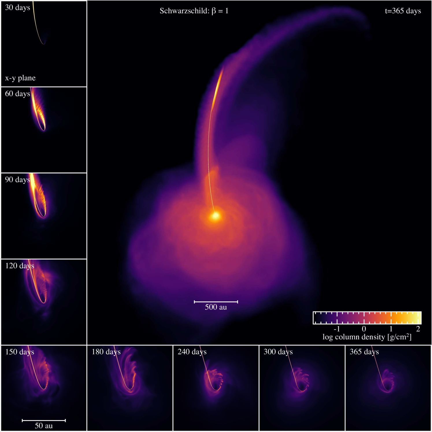
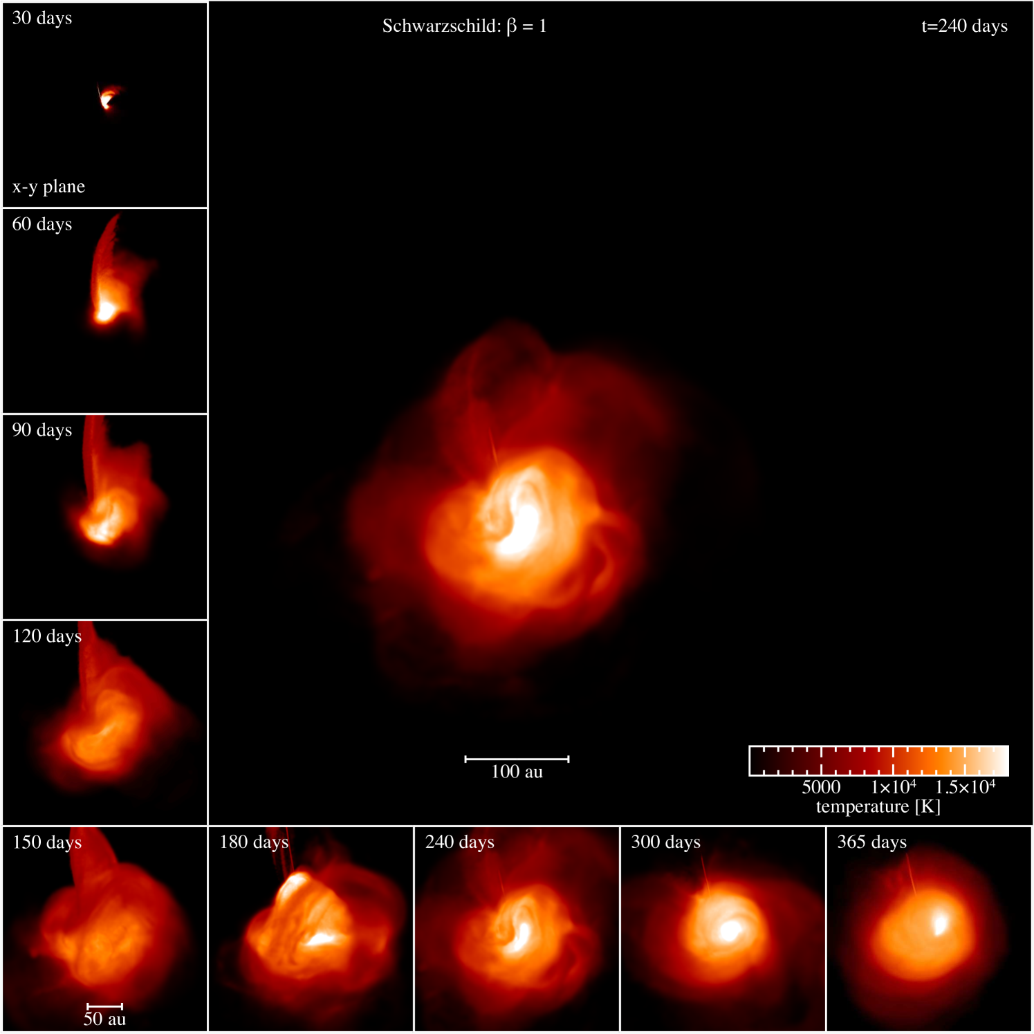
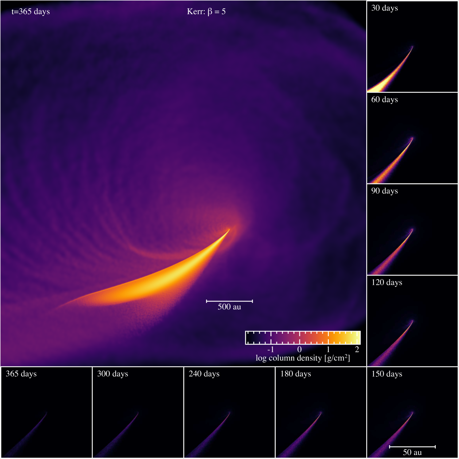
Figure 1 shows snapshots of the long-term debris evolution in the , high-resolution, adiabatic simulation with a non-rotating black hole. The star takes approximately 7 hours to reach pericentre at which point it is tidally disrupted and forms a long, thin debris stream. Approximately half of the stream is bound to the black hole while the other half is unbound (visible as the thin, dense upward stream in the figure). The head of the stream (i.e., the most bound material) takes 26 days to return to pericentre. After the stream passes through pericentre for a second time, the small amount of apsidal precession leads to stream self-intersection at the ‘outer shock’ (most evident in inset panels shown at 60 and 90 days; see Appendix B for more detail on the outer shock), which cause material to eventually fall towards the black hole, driving the formation of kinetic outflows which spread almost isotropically, eventually encasing the black hole (main panel). A fraction of the material joins the returning debris and returns to pericentre, however most of it goes into a low density mechanical outflow. Following the fallback for one year post disruption, we find that the bubble continues to expand, with only a small amount of material forming an eccentric disc (lower panels of Figure 1). The large-scale debris structure (main panel) is similar to the ‘Eddington envelope’ first proposed by Loeb & Ulmer (1997) except that ours is outflowing rather than static, as predicted by subsequent authors (Strubbe & Quataert, 2009; Jiang et al., 2016; Metzger & Stone, 2016).
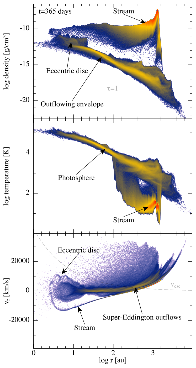
Figure 2 shows the density (top), temperature (middle) and radial velocity (bottom) distributions of particles a year after disruption, with temperature calculated from Equation (3). The density of the outflowing envelope is g cm-3, approximately six orders of magnitude lower than the density of the stream, which is g cm-3. The typical outflow velocity is 104 km s-1. After one year there is approximately 67% ( M⊙) of the stellar mass in the incoming or unbound stream, 31.2% ( M⊙) in the envelope, 0.8% ( M⊙) in the eccentric disc, while 1% ( M⊙) has been accreted by the black hole.
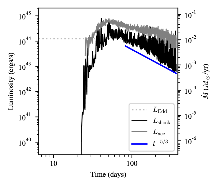
The top panel of Figure 3 shows the energy dissipation rate in our simulation, . This was computed by computing the time derivative of the thermal energy caused by irreversible heating terms due to viscosity and shocks. We find that it is dominated by regions close the accretion radius . The energy dissipation rate rises rapidly from 26 days, when accretion begins, until 50 days after disruption when it reaches a peak of erg s-1 (roughly the Eddington limit). This is followed by a power law decay that does approximately match the expected energy dissipation from the mass fallback rate (Rees, 1988; Phinney, 1989), but with lower than the mass fallback rate by approximately two orders of magnitude. We compare this to the luminosity derived from our measured mass accretion rate , given by . Here, is the efficiency based on our inner accretion radius. However, since our is inside the last stable orbit, matter crossing this radius is mostly advected into the black hole rather than radiated, so converting it into a luminosity simply measures the amount of energy that would have been dissipated to reach this radius if all the matter were on a perfectly circular orbit. The resulting ‘luminosity’ follows the same trend as the actual energy dissipation rate above, but is 0.5–1 orders of magnitude greater throughout the simulation. This suggests some material is accreted almost radially, with little to no orbital energy dissipated before accretion (Svirski et al., 2017).
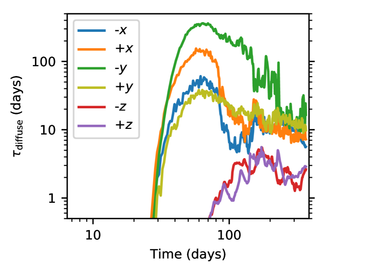
The lower panel of Figure 3 shows the approximate time taken for photons to diffuse from near the black hole out to the photosphere radius, assuming the material remains static. We computed this via
| (6) |
by summing the contributions from each SPH particle intersecting a line-of-sight along each coordinate axis with opacity cm2/g. The typical photon diffusion time varies between 10–200 days, peaking approximately 80 days after disruption and decaying roughly as a power law. This indicates that, although most energy is dissipated in regions close to the black hole (see Figure 9), where the reservoir of gravitational binding energy is largest, this material is optically thick. The energy is transported outward by mechanical outflows before some of it is radiated through a photosphere.
Figure 4 shows the temperature at the ‘photosphere’ of the outflowing envelope, produced by ray-tracing through our simulation as described in Sec. 2.1. An expanding emission region of 10–100 au is consistent with those inferred from TDE observations (van Velzen et al., 2021). Photospheric temperatures are in the range expected to produce blackbody emission at UV/optical wavelength. Figure 2 shows that temperatures would remain in the 104–105 K range even accounting for scattering from deeper layers (see Appendix C).
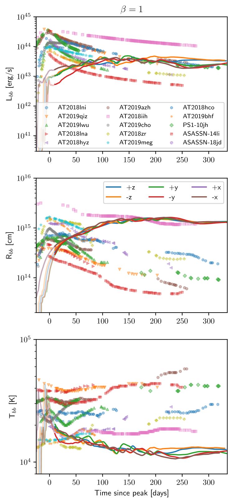
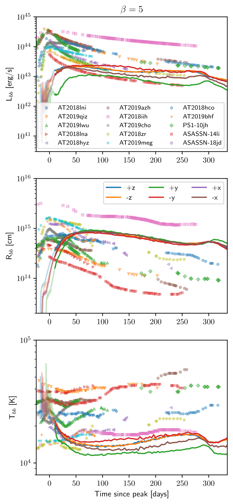
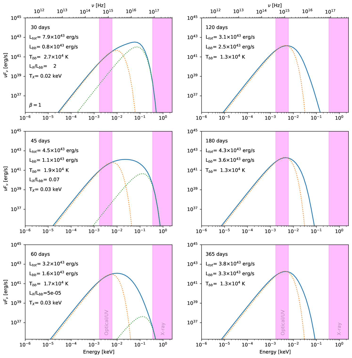
Figure 5 compares the corresponding time evolution of our measured , and (inferred bolometric luminosity, blackbody radius and temperature of the blackbody fit to optical wavelengths, respectively) from six different lines of sight (solid lines) to the evolution of observed TDEs inferred from black body fits taken from van Velzen et al. (2021) and Neustadt et al. (2020) (dots). The equivalent plot for the more penetrating encounter is shown on the right.
The typical luminosity (top panel) is around – erg s-1 (– ), however we caution that the exact value is sensitive to our photospheric temperature (since ). Nonetheless, our approximate luminosities are consistent with the observed values (see figure 9 of Holoien et al. 2019), as well as with the analytically computed light curves of Lodato & Rossi (2011) (see left panel of their Figure 7). The bolometric luminosity of the envelope in our models appears almost constant, and close to the Eddington value, key features of the analytical model of Loeb & Ulmer (1997).
The photospheric radius (centre panels), when computed by fitting to synthetic spectra in the optical band (Appendix C), is relatively insensitive to the line-of-sight, giving typical radii of 10–100 au (– cm), in the same range as the observations. The photospheric radius reaches a peak after roughly 150–200 days in the calculation, and days in the calculation, the latter more closely matching the typical day rise time seen in most of the observations. On the other hand some TDE candidates such as ASASSN-18jd (Neustadt et al., 2020) (see legend) do show a more or less flat luminosity evolution over a 1 yr timescale, similar to our lightcurves. The transients AT2018hco and AT2019iih show the closest match to the photospheric radius evolution in our calculation, particularly for days.
We find photospheric temperatures (lower panels) in the range of –, with the same range as the observations, but with slightly lower temperatures in our models (K) compared to the observations (–K) for days. This may be a result of our underestimate of the photospheric temperature due to scattering of photons from deeper layers (Appendix C). The observed trend of temperatures slowly rising as a function of time for days is reproduced in our calculation (right panels of Figure 5). Our temperature evolution is similar to that obtained by Mockler et al. (2019) who fitted models of a ‘dynamic reprocessing layer’ to observed TDEs (see their Figure 8), finding a 10–20 day sharp rise in temperature followed by a dip and subsequent flat or slowly rising evolution.
A notable feature in both the and cases are the almost flat lightcurves predicted at late times along most lines of sight. This is also observed (e.g. Holoien et al., 2019; van Velzen et al., 2021). In our simulations this corresponds to the stalling of the photospheric radii in an expanding gas cloud; however, as discussed below, models without cooling may not accurately describe light curves after year.
Discussion
Our simulations address the main challenge of tidal disruption events: to simulate the disruption of a star, on a parabolic orbit, by a black hole in general relativity, and to model the subsequent accretion flow from first principles.
Our main new insight from doing so is that, as in Hu et al. (2024), we have been able to self-consistently form the hypothesised ‘Eddington envelope’ for the first time, more or less as predicted by Loeb & Ulmer (1997) and Metzger & Stone (2016). With the disrupted star moving on an orbit with a mean energy of zero and low angular momentum, we found dissipation of energy and angular momentum to occur through relativistic precession and ensuing stream-stream collisions (see Appendix A), as found by previous authors for stars on bound trajectories (Hayasaki et al., 2016; Bonnerot et al., 2016; Stone et al., 2019; Liptai et al., 2019) and similar to the process originally envisioned by Rees (1988).
Once accretion commences in the optically thick environment with inefficient cooling (we assumed adiabatic gas), the gravitational energy of accreting material launches mechanical outflows, yielding a large, asymmetric, optically thick outflowing envelope (Fig. 4).
We found a similar outflow in recent calculations of initially eccentric encounters (Hu et al., 2024), but with faster rise of the lightcurve due to the shorter orbital periods. The main difference in the parabolic case is that only of the star is accreted, compared to more than half the star for the eccentric encounters (Hu et al., 2024). The lower efficiency of accretion occurs because of the smaller amount of bound material reaching the inner regions (Appendix A).
The envelope structure is similar to other rapidly expanding, optically thick, quasi-spherical outflows powered by a central energy source, such as supernovae and kilonovae. In this case, the expanding envelope is powered by gravitational energy, dissipated in the radiatively inefficient accretion flow onto the black hole (see Figure 9). Our black hole mass accretion rate, shown in Figure 3, is 1–1.5 orders of magnitude lower than the predicted mass fallback rate. This broad conclusion on the formation of an Eddington envelope is unchanged by whether or not the black hole is spinning, or by whether the star approaches closer to the black hole (see Figure 11), or the numerical resolution (see Appendix E).
That our outflowing envelope, or ‘Black Hole Sun’, is optically thick is demonstrated by our estimated photon diffusion timescales of 10–100 days shown in the bottom panel of Figure 3. This means that the debris produced by the disruption cannot cool efficiently, leading to the formation of a photosphere. Synthetic spectral energy distributions (Appendix C) show this leads to ratios of optical to X-ray emission of order –, similar to those observed (van Velzen et al., 2021).
Our numerical experiments have several serious limitations in how well they represent real tidal disruptions. The main ones are that we employed an adiabatic approximation, meaning that none of the energy produced is actually radiated in our simulations, that we assume and used a polytrope not a real star.
Our adiabatic assumption is likely a good approximation near the peak of the light curve since the photon diffusion timescale is long, although it does not account for the change to the radiation-pressure dominated regime after shock heating, which implies that the adiabatic index should change to . On the other hand, the adiabatic assumption likely breaks down by around 1 year after disruption. At t 1 yr, our estimated luminosity (Figure 5) becomes comparable to the energy input rate from shock heating (Figure 3), while the photon diffusion timescale becomes comparable to the time for the kinetic outflows to reach the photosphere, allowing material to radiatively cool.
Therefore, at t 1 yr, with relatively efficient diffusion, the observable luminosity should transition to tracking the shock heating rate, which in turn roughly tracks the mass return rate with scaling (top panel of Figure 3). Efficient cooling after 1 year may also lead to thin disc formation (see Appendix A), rather than the eccentric thick disc formed at days in Figure 1. Cooling may also cause our photospheres to retreat at later times, better matching the photospheric radius and temperature observations.
Despite this limitation, our photospheric radius estimates yield a luminosity evolution with the same order of magnitude as optical/UV light curves from several recently observed TDEs (see Figure 5). We do not expect that the dynamics of our simulations would be significantly affected by allowing the photosphere to radiate at early times, mainly because the energy release via radiation is small — most of the energy in our Eddington envelope is released via mechanical outflows, with typical outflow velocities of 1–2 km s-1 (see bottom panel of Figure 2). Such velocities match those observed in spectral lines (e.g. Leloudas et al., 2019).
We find that the optical light curve is sensitive to the observing angle, as suggested by Dai et al. (2018a), but due to different photospheric temperatures along different lines of sight (see Figure 5) rather than the presence of a disc. Mildly supersonic outflows indicate that temperatures are not in equilibrium across the photosphere.
The photospheric radii plateau at to au, depending on the line of sight and the amount of material participating in the outflow (Figure 5). Applying a single-zone model with uniform density to a homologously expanding envelope, this stalling is estimated to occur when the photospheric radius is , where the mass in the envelope depends on the penetration factor . This estimate yields a photospheric radius plateau of au for our choice of and . While our predicted radius evolution might change if we allowed radiation to escape (especially at these late times), a significant late-time flattening has been observed in optical/UV for black holes of this mass (van Velzen et al., 2019).
Many TDE candidates show soft X-ray emission. While in general the ratio of X-ray to optical luminosities in TDE is low (Auchettl et al., 2017), there are cases where optical and X-ray emission are both present. ASASSN-14li has similar X-ray and optical luminosities (Holoien et al., 2016), though with X-rays lagging by 32 days (Pasham et al., 2017), which is difficult to explain via reprocessing. Our model can help to explain some of these TDE features. At late times, as the material cools and the photosphere retreats to reveal regions close to the black hole, we expect the formation of a disc or a thick torus similar to that described in Appendix A, which will be a significant central X-ray source.
Indeed, we found in our calculation (Appendix C) that retreat of the photosphere produces a rising X-ray luminosity similar to some observed TDEs Gezari et al. (2017) and to the class of ‘veiled’ TDEs (Auchettl et al., 2017). Our Eddington envelope naturally obscures any central X-ray source, with absorption strongly varying for different lines of sight with typical – cm-2. This suggests an explanation for the dichotomy between X-ray and optical TDE in terms of different viewing angles to the source, in a sort of ‘unified’ model for TDE emission (Dai et al., 2018b).
4 Conclusions
In summary, we simulated the tidal disruption of 1M⊙ polytropic stars around a solar mass black hole, using general relativistic hydrodynamics in the Kerr metric, following the simulations for one year post disruption. Our main finding, similar to our recent finding for real stars on eccentric orbits (Hu et al., 2024) is the production of an optically thick ‘Eddington envelope’ hypothesised by previous authors (e.g. Loeb & Ulmer, 1997; Metzger & Stone, 2016). Our calculations predict:
-
1.
outflow velocities of km s-1;
-
2.
large photosphere radii of – au;
-
3.
a relatively low mass accretion rate (yr) mediated by the mechanical outflow of material;
-
4.
peak luminosities of – erg/s.
We find that our encounters provide a better match to TDE observations than , and that black hole spin does not significantly change the outcome. We thus confirm Eddington envelopes as the likely solution to the puzzle of TDE optical/UV emission.
References
- Abramowicz et al. (1991) Abramowicz, M. A., Novikov, I. D., & Paczynski, B. 1991, ApJ, 369, 175, doi: 10.1086/169748
- Andalman et al. (2022) Andalman, Z. L., Liska, M. T. P., Tchekhovskoy, A., Coughlin, E. R., & Stone, N. 2022, MNRAS, 510, 1627, doi: 10.1093/mnras/stab3444
- Arcavi et al. (2014) Arcavi, I., Gal-Yam, A., Sullivan, M., et al. 2014, ApJ, 793, 38. https://arxiv.org/abs/1405.1415
- Auchettl et al. (2017) Auchettl, K., Guillochon, J., & Ramirez-Ruiz, E. 2017, ApJ, 838, 149. https://arxiv.org/abs/1611.02291
- Ayal et al. (2000) Ayal, S., Livio, M., & Piran, T. 2000, ApJ, 545, 772
- Bonnerot & Lu (2020) Bonnerot, C., & Lu, W. 2020, MNRAS, 495, 1374, doi: 10.1093/mnras/staa1246
- Bonnerot & Lu (2022) —. 2022, MNRAS, 511, 2147, doi: 10.1093/mnras/stac146
- Bonnerot et al. (2016) Bonnerot, C., Rossi, E. M., & Lodato, G. 2016, MNRAS, 458, 3324. https://arxiv.org/abs/1511.00300
- Bonnerot et al. (2016) Bonnerot, C., Rossi, E. M., Lodato, G., & Price, D. J. 2016, MNRAS, 455, 2253
- Calderón et al. (2024) Calderón, D., Pejcha, O., Metzger, B. D., & Duffell, P. C. 2024, MNRAS, 528, 2568, doi: 10.1093/mnras/stae194
- Chornock et al. (2014) Chornock, R., Berger, E., Gezari, S., et al. 2014, ApJ, 780, 44. https://arxiv.org/abs/1309.3009
- Coughlin & Begelman (2014) Coughlin, E. R., & Begelman, M. C. 2014, ApJ, 781, 82, doi: 10.1088/0004-637X/781/2/82
- Dai et al. (2018a) Dai, L., McKinney, J. C., Roth, N., Ramirez-Ruiz, E., & Miller, M. C. 2018a, ApJ, 859, L20. https://arxiv.org/abs/1803.03265
- Dai et al. (2018b) —. 2018b, ApJ, 859, L20, doi: 10.3847/2041-8213/aab429
- Diener et al. (1997) Diener, P., Frolov, V. P., Khokhlov, A. M., Novikov, I. D., & Pethick, C. J. 1997, ApJ, 479, 164
- Evans & Kochanek (1989) Evans, C. R., & Kochanek, C. S. 1989, ApJ, 346, L13
- Frolov et al. (1994) Frolov, V. P., Khokhlov, A. M., Novikov, I. D., & Pethick, C. J. 1994, ApJ, 432, 680
- Gafton & Rosswog (2019) Gafton, E., & Rosswog, S. 2019, arXiv e-prints. https://arxiv.org/abs/1903.09147
- Gezari et al. (2017) Gezari, S., Cenko, S. B., & Arcavi, I. 2017, ApJ, 851, L47. https://arxiv.org/abs/1712.03968
- Gezari et al. (2012) Gezari, S., Chornock, R., Rest, A., et al. 2012, Nature, 485, 217. https://arxiv.org/abs/1205.0252
- Goicovic et al. (2019) Goicovic, F. G., Springel, V., Ohlmann, S. T., & Pakmor, R. 2019, MNRAS, 487, 981. https://arxiv.org/abs/1902.08202
- Golightly et al. (2019) Golightly, E. C. A., Coughlin, E. R., & Nixon, C. J. 2019, The Astrophysical Journal, 872, 163. https://arxiv.org/abs/1901.03717
- Guillochon et al. (2014) Guillochon, J., Manukian, H., & Ramirez-Ruiz, E. 2014, ApJ, 783, 23. https://arxiv.org/abs/1304.6397
- Guillochon & Ramirez-Ruiz (2013) Guillochon, J., & Ramirez-Ruiz, E. 2013, ApJ, 767, 25. https://arxiv.org/abs/1206.2350
- Guillochon et al. (2009) Guillochon, J., Ramirez-Ruiz, E., Rosswog, S., & Kasen, D. 2009, ApJ, 705, 844. https://arxiv.org/abs/0811.1370
- Hatfull et al. (2021) Hatfull, R. W. M., Ivanova, N., & Lombardi, J. C. 2021, MNRAS, 507, 385, doi: 10.1093/mnras/stab2140
- Hayasaki et al. (2013) Hayasaki, K., Stone, N., & Loeb, A. 2013, MNRAS, 434, 909. https://arxiv.org/abs/1210.1333
- Hayasaki et al. (2016) —. 2016, MNRAS, 461, 3760. https://arxiv.org/abs/1501.05207
- Holoien et al. (2016) Holoien, T. W. S., Kochanek, C. S., Prieto, J. L., et al. 2016, MNRAS, 455, 2918. https://arxiv.org/abs/1507.01598
- Holoien et al. (2019) Holoien, T. W. S., Huber, M. E., Shappee, B. J., et al. 2019, ApJ, 880, 120. https://arxiv.org/abs/1808.02890
- Hu et al. (2024) Hu, F. F., Price, D. J., & Mandel, I. 2024, ApJ, 963, L27, doi: 10.3847/2041-8213/ad29ec
- Huang et al. (2023) Huang, X., Davis, S. W., & Jiang, Y.-f. 2023, ApJ, 953, 117, doi: 10.3847/1538-4357/ace0be
- Jiang et al. (2016) Jiang, Y.-F., Guillochon, J., & Loeb, A. 2016, ApJ, 830, 125. https://arxiv.org/abs/1603.07733
- Kerr (1963) Kerr, R. P. 1963, Physical Review Letters, 11, 237
- Kesden (2012) Kesden, M. 2012, Phys. Rev. D, 86, 064026. https://arxiv.org/abs/1207.6401
- Khokhlov et al. (1993) Khokhlov, A., Novikov, I. D., & Pethick, C. J. 1993, ApJ, 418, 181
- Kobayashi et al. (2004) Kobayashi, S., Laguna, P., Phinney, E. S., & Mészáros, P. 2004, ApJ, 615, 855
- Laguna et al. (1993) Laguna, P., Miller, W. A., & Zurek, W. H. 1993, ApJ, 404, 678
- Law-Smith et al. (2019) Law-Smith, J., Guillochon, J., & Ramirez-Ruiz, E. 2019, ApJ, 882, L25, doi: 10.3847/2041-8213/ab379a
- Leloudas et al. (2019) Leloudas, G., Dai, L., Arcavi, I., et al. 2019, arXiv e-prints, arXiv:1903.03120. https://arxiv.org/abs/1903.03120
- Liptai & Price (2019) Liptai, D., & Price, D. J. 2019, MNRAS, 485, 819. https://arxiv.org/abs/1901.08064
- Liptai et al. (2019) Liptai, D., Price, D. J., Mandel, I., & Lodato, G. 2019, arXiv e-prints, arXiv:1910.10154. https://arxiv.org/abs/1910.10154
- Lodato (2012) Lodato, G. 2012, in European Physical Journal Web of Conferences, Vol. 39, European Physical Journal Web of Conferences, 01001. https://arxiv.org/abs/1211.6109
- Lodato et al. (2009) Lodato, G., King, A. R., & Pringle, J. E. 2009, MNRAS, 392, 332. https://arxiv.org/abs/0810.1288
- Lodato & Rossi (2011) Lodato, G., & Rossi, E. M. 2011, MNRAS, 410, 359. https://arxiv.org/abs/1008.4589
- Loeb & Ulmer (1997) Loeb, A., & Ulmer, A. 1997, ApJ, 489, 573. https://arxiv.org/abs/astro-ph/9703079
- Matsumoto & Metzger (2022) Matsumoto, T., & Metzger, B. D. 2022, ApJ, 938, 5, doi: 10.3847/1538-4357/ac6269
- Metzger (2022) Metzger, B. D. 2022, ApJ, 937, L12, doi: 10.3847/2041-8213/ac90ba
- Metzger & Stone (2016) Metzger, B. D., & Stone, N. C. 2016, Monthly Notices of the Royal Astronomical Society, 461, 948. https://arxiv.org/abs/1506.03453
- Miller (2015) Miller, M. C. 2015, ApJ, 805, 83. https://arxiv.org/abs/1502.03284
- Mockler et al. (2019) Mockler, B., Guillochon, J., & Ramirez-Ruiz, E. 2019, ApJ, 872, 151. https://arxiv.org/abs/1801.08221
- Nealon et al. (2015) Nealon, R., Price, D. J., & Nixon, C. J. 2015, MNRAS, 448, 1526
- Neustadt et al. (2020) Neustadt, J. M. M., Holoien, T. W. S., Kochanek, C. S., et al. 2020, MNRAS, 494, 2538, doi: 10.1093/mnras/staa859
- Nicholl et al. (2019) Nicholl, M., Blanchard, P. K., Berger, E., et al. 2019, MNRAS, 488, 1878, doi: 10.1093/mnras/stz1837
- Nixon et al. (2012) Nixon, C., King, A., Price, D., & Frank, J. 2012, ApJ, 757, L24. https://arxiv.org/abs/1209.1393
- Ogura & Fukue (2013) Ogura, K., & Fukue, J. 2013, PASJ, 65, 92, doi: 10.1093/pasj/65.4.92
- Pasham et al. (2017) Pasham, D. R., Cenko, S. B., Sadowski, A., et al. 2017, ApJ, 837, L30. https://arxiv.org/abs/1703.07024
- Pasham et al. (2019) Pasham, D. R., Remillard, R. A., Fragile, P. C., et al. 2019, Science, 363, 531, doi: 10.1126/science.aar7480
- Patra et al. (2022) Patra, K. C., Lu, W., Brink, T. G., et al. 2022, MNRAS, 515, 138, doi: 10.1093/mnras/stac1727
- Phinney (1989) Phinney, E. S. 1989, in IAU Symposium, Vol. 136, The Center of the Galaxy, ed. M. Morris, 543
- Piran et al. (2015) Piran, T., Svirski, G., Krolik, J., Cheng, R. M., & Shiokawa, H. 2015, ApJ, 806, 164. https://arxiv.org/abs/1502.05792
- Price (2007) Price, D. J. 2007, PASA, 24, 159. https://arxiv.org/abs/0709.0832
- Price et al. (2018) Price, D. J., Wurster, J., Tricco, T. S., et al. 2018, PASA, 35, e031. https://arxiv.org/abs/1702.03930
- Ramirez-Ruiz & Rosswog (2009) Ramirez-Ruiz, E., & Rosswog, S. 2009, ApJ, 697, L77. https://arxiv.org/abs/0808.3847
- Rees (1988) Rees, M. J. 1988, Nature, 333, 523
- Rosswog et al. (2008) Rosswog, S., Ramirez-Ruiz, E., Hix, W. R., & Dan, M. 2008, Computer Physics Communications, 179, 184. https://arxiv.org/abs/0801.1582
- Roth et al. (2016) Roth, N., Kasen, D., Guillochon, J., & Ramirez-Ruiz, E. 2016, ApJ, 827, 3. https://arxiv.org/abs/1510.08454
- Ryu et al. (2023) Ryu, T., Krolik, J., Piran, T., Noble, S. C., & Avara, M. 2023, ApJ, 957, 12, doi: 10.3847/1538-4357/acf5de
- Sacchi & Lodato (2019) Sacchi, A., & Lodato, G. 2019, MNRAS, 486, 1833. https://arxiv.org/abs/1904.02424
- Sadowski et al. (2016) Sadowski, A., Tejeda, E., Gafton, E., Rosswog, S., & Abarca, D. 2016, MNRAS, 458, 4250
- Steinberg & Stone (2024) Steinberg, E., & Stone, N. C. 2024, Nature, 625, 463, doi: 10.1038/s41586-023-06875-y
- Stella & Vietri (1998) Stella, L., & Vietri, M. 1998, ApJ, 492, L59, doi: 10.1086/311075
- Stone et al. (2019) Stone, N. C., Kesden, M., Cheng, R. M., & van Velzen, S. 2019, General Relativity and Gravitation, 51, 30. https://arxiv.org/abs/1801.10180
- Strubbe & Quataert (2009) Strubbe, L. E., & Quataert, E. 2009, MNRAS, 400, 2070. https://arxiv.org/abs/0905.3735
- Svirski et al. (2017) Svirski, G., Piran, T., & Krolik, J. 2017, MNRAS, 467, 1426. https://arxiv.org/abs/1508.02389
- Tejeda et al. (2017) Tejeda, E., Gafton, E., Rosswog, S., & Miller, J. C. 2017, MNRAS, 469, 4483. https://arxiv.org/abs/1701.00303
- van Velzen (2018) van Velzen, S. 2018, ApJ, 852, 72. https://arxiv.org/abs/1707.03458
- van Velzen et al. (2019) van Velzen, S., Stone, N. C., Metzger, B. D., et al. 2019, ApJ, 878, 82. https://arxiv.org/abs/1809.00003
- van Velzen et al. (2011) van Velzen, S., Farrar, G. R., Gezari, S., et al. 2011, ApJ, 741, 73. https://arxiv.org/abs/1009.1627
- van Velzen et al. (2021) van Velzen, S., Gezari, S., Hammerstein, E., et al. 2021, ApJ, 908, 4, doi: 10.3847/1538-4357/abc258
Appendix A Radiatively efficient cooling and disc formation
Figure 6 demonstrates that disc formation can occur more rapidly if the gas is allowed to cool. We performed a medium-resolution simulation with the same parameters as in Fig. 1 but using an isentropic approximation in which we discard all irreversible heating due to viscosity and shocks, but retain heating and cooling due to work; see Liptai et al. 2019). This shows that a compact, circularised disc can more efficiently form if the stream remains cold. The formation process is similar to the stream-stream collisions seen in simulations of tidally disrupted stars on bound orbits (Hayasaki et al., 2016; Bonnerot et al., 2016) caused by the general relativistic orbital precession (Rees, 1988), except that the collisions occur at relatively large distances from the black hole (s of au) for our encounter. No optically thick envelope is formed in the isentropic case as the main energy source is switched off.
The second panel of Figure 6 quantifies the degree of relativistic apsidal precession, plotting three sample trajectories computed by integrating the geodesic equations111https://github.com/phantomSPH/phantom-geodesic for three sample particles in the returning debris stream with (solid lines), which may be compared to the corresponding Newtonian trajectories (dashed lines). The relativistic precession, while small for , nevertheless leads to self-intersection of the stream and hence disc formation.
Figure 7 shows the same calculation but performed with a spinning black hole (; ). The disc formation process can be seen to occur in a similar manner. The second panel shows the same set of orbital trajectories as in Figure 6, but computed with . These are indistinguishable from those shown in Figure 6, indicating that the spin does not play a large role in the disc formation process for encounters. The main difference is that in the case of a spinning black hole, the disc that is subsequently formed undergoes differential Lense-Thirring precession leading to disc tearing as predicted by Nixon et al. (2012) and Nealon et al. (2015). Such differentially precessing rings are thought to be responsible for Quasi-Periodic Oscillations in black hole accretion discs (Stella & Vietri, 1998) and are also observed in tidal disruption events (Pasham et al., 2019).
This approximation of efficient cooling throughout the disruption event is unrealistic. Hence we also performed an additional numerical experiment where we continued the medium-resolution adiabatic calculation (with the same parameters as Fig. 1) but at 1 year after disruption switched to an isentropic formulation. This corresponds to roughly the time when the photon diffusion time becomes short (Fig. 3 bottom) and the adiabatic cooling rate exceeds the energy dissipation rate. However, in reality, the envelope would transition smoothly from nearly adiabatic expansion with inefficient cooling to efficient radiative cooling represented by the isentropic model. That we also form a circularised disc in this experiment confirms that a disc would efficiently form even at low resolution if material was allowed to cool.
Appendix B Thermodynamics
Our adiabatic simulations show lateral expansion of the stream in the nozzle shock that occurs during second periapsis passage compared to isentropic calculations. Material in the returning stream, with a narrow range of energies and angular momenta, is spread out along a range of trajectories because of heating through the nozzle shock. Some of the nozzle shock heating is overestimated, especially at low numerical resolution (see Figure 13). However, provided the Mach number remains high then material continues to follow the precessing geodesic orbits similar to those shown in Figure 6. Figure 9 shows the line-of-sight averaged internal energy in our highest resolution calculation (as shown in Figure 1). As the right panel of Figure 9 shows, the Mach number drops to around 50 after the nozzle shock in our highest resolution calculation, which is sufficient to continue mostly along a geodesic trajectory.
More important to the circularisation process is the ‘outer shock’ due to self-intersection of the stream near apoapsis, labelled as ‘stream-stream collision’ in the figure. Here, the Mach number drops to approximately unity in the shocked material (see right panel of Figure 9). Such material is then sprayed on a broad range of trajectories (as per Figure 14), in particular providing the ‘cold accretion flow’ (see labels in Figure 9) towards the black hole, enabling prompt accretion, similar to the process envisioned by Bonnerot & Lu (2020).
The process of stream-stream collisions initiating the accretion flow towards the black hole is similar to that which occurs in isentropic calculations (Appendix A). The main difference in the adiabatic simulations is that material reaching the inner regions close to the black hole no longer remains cold, with the additional heating producing kinetic outflows (Figure 9).
Appendix C Photospheric evolution
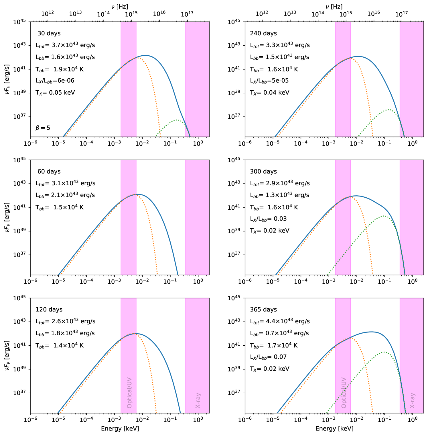
Figure 10 shows our synthetic spectral energy distributions (SEDs) at selected times (see legend) for the calculation. The overall spectrum is non-thermal, with significant excess at high energies compared to the optical blackbody fit (orange dotted curve; computed by fitting a single temperature blackbody to the optical band using scipy.optimize.curve_fit). The high energy excess can be seen to produce soft X-rays whenever emission from the inner regions is visible. In the calculation this occurs for days, before the Eddington envelope smothers the central engine (see corresponding panels in Figure 4).
While our predicted ratios of optical to X-ray emission of 1 to are similar to those observed, we find our predicted X-ray emission depends on . Observations also show slightly higher X-ray temperatures in the range keV (van Velzen et al., 2021) and tend to find X-ray luminosities that increase with time. Figure 12 shows that something close to this occurs for the calculation. Here the more extreme precession leads to rapid smothering of the central engine in days, but the faster stream dynamics means that the photosphere undergoes a visible retreat at days (see Figure 5) leading to increasing X-ray emission for days in the case where the star penetrates deeper.
Appendix D Effect of penetration factor
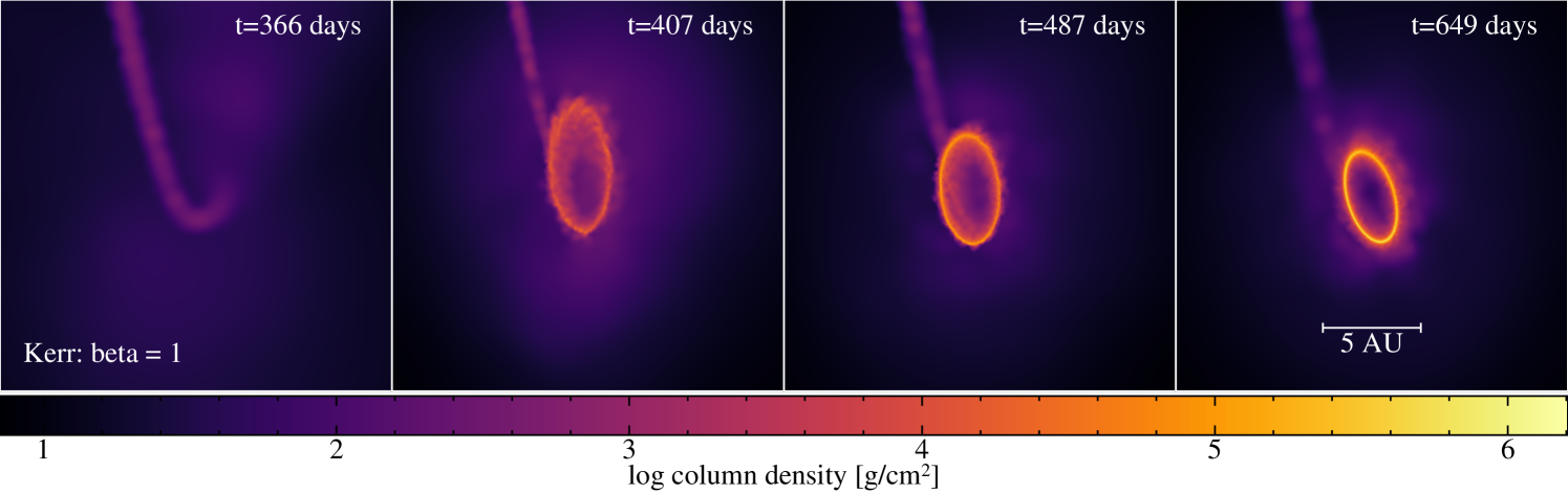
Figure 11 shows snapshots of the debris fallback for a calculation with an increased penetration factor of , for a Kerr black hole with with the initial orbit inclined by 60∘ with respect to the black hole spin plane.
Since the star approaches much closer to the black hole, the effects of apsidal and Lense-Thirring precession throw the star/debris stream into an orbital plane that is different to the initial one. This changes the debris geometry projected in each coordinate plane, however the overall picture remains unchanged. That is, the returning debris stream feeds the expansion of a low density Eddington envelope as in the case. Circularisation of the debris stream is faster in our calculation because of the enhanced general relativistic precession, resulting in more prompt envelope formation (Figure 11).
The right panel of Figure 5 shows the corresponding lightcurves for this calculation (discussed in the main text), while Figure 12 shows the corresponding spectral energy distributions.
Appendix E Effect of resolution
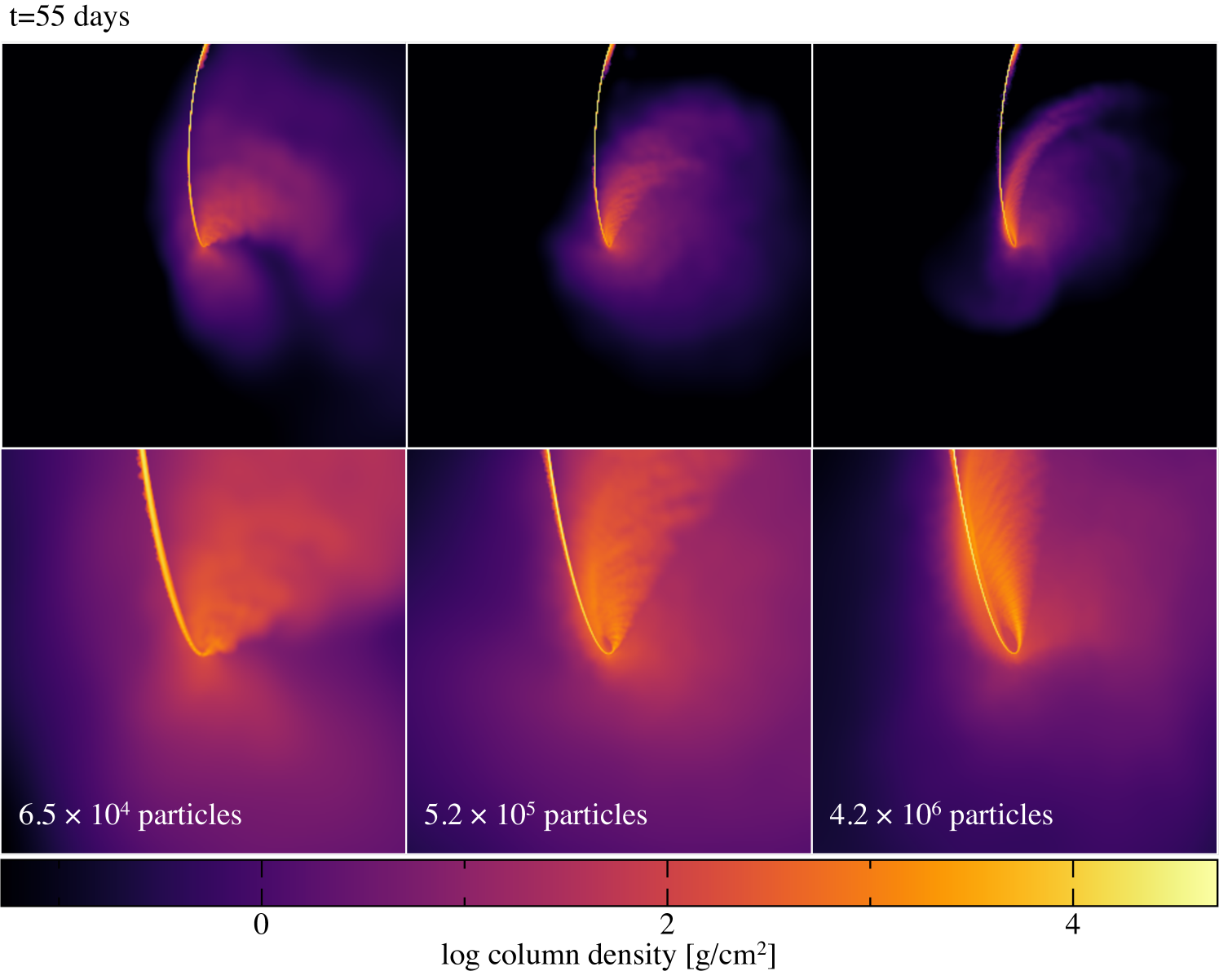
Figure 13 shows the effect of resolution in our simulations. The setup is identical to that shown in Figure 1. The top row compares the large scale structure, while the bottom compares the details of the stream on a smaller scale as it passes through the nozzle shock. We increased the number of particles by approximately a factor of 8 between each column from left to right, corresponding to a factor of 2 increase in spatial resolution. We find that heating through the nozzle shock is overestimated at low numerical resolutions, leading to a more isotropic outflow. While the degree of nozzle shock heating is not fully converged even at our highest resolution (as expected from Bonnerot & Lu 2022), the Mach number remains sufficiently high that the material mostly follows colder trajectories along orbital geodesics as in the isentropic case (see Figure 6). Hence the process of circularisation tends towards being driven mainly by the stream self-intersection at apocentre rather than nozzle shock heating at pericentre which is dominant at low resolution. Our results also imply that the envelope may be less isotropic in reality, with more material in a ‘spiral arm’ that is denser than the rest of the envelope.
To clarify the numerical dependence of the lateral stream expansion in the nozzle shock we performed two additional numerical experiments. The first involved a simple injection of material at different Mach numbers into an otherwise empty domain with no central black hole. We chose parameters typical of those observed in the tidal disruption calculations, by injecting material in a stream at the typical location of the returning stream just prior to pericenter in our calculations, namely at in geometric units. We fixed the injection velocity to be the incoming stream velocity observed in our simulations, namely at where is the pericenter distance for the original star, at . We injected a stream as a cylinder of particles with a radius of and varied the Mach number of the stream (by setting the incoming thermal energy ). Particles were placed in a cubic lattice arrangement, cropped to the radius of the cylinder. Calculations were performed with an adiabatic equation of state with . We adopted a resolution of 16 particles per stream width, giving 565,940 particles in the domain at . The mass of the SPH particles is arbitrary for this problem (we chose ) and we employed the non-relativistic version of Phantom for simplicity.
Figure 14 shows the results of this experiment. The lateral expansion of the stream can be seen to be a simple function of the Mach number of the flow. Below Mach 10 significant lateral expansion of the stream may be observed. We found the degree of lateral expansion to be independent of both the injected stream width and the numerical resolution, depending solely on the Mach number.
Our second experiment was the same but with a point mass placed at the origin with to capture the pericenter dynamics. Since we injected material with a finite width but a single velocity the infinite Mach number orbital trajectories of the highly eccentric orbits cause a ‘traffic jam’ at pericenter which induces PdV work on the stream. We adopted an initial Mach number of 50, consistent with that measured from our tidal disruption calculations, but set the initial radius of the injected stream to and , respectively. Apart from the overall drop in density as the stream width is increased, the lateral expansion of the stream remained the same in all cases. This demonstrates that an artificially wide or unresolved stream width is not the main cause of the lateral expansion.
Figure 13 shows the post-pericentre Mach number drop is overestimated at low resolution due to excess heating in the nozzle shock, leading to an overestimated stream width. The qualitative behaviour is unchanged so long as the post-pericentre Mach number remains high, as occurs in our highest resolution adiabatic calculations, and isentropic calculations at all resolutions.
Conservation properties are well preserved by the numerical scheme at all resolutions. For example, in the calculation shown in Figure 1 the energy error is up to days when accretion commences, after which the total energy rises steadily due to the removal of accreted mass with negative specific energy from the simulation. Total angular momentum is conserved to (0.02%) over the entire 365 days of the simulation.