Edge Augmentation with Controllability Constraints in
Directed Laplacian Networks
Abstract
In this paper, we study the maximum edge augmentation problem in directed Laplacian networks to improve their robustness while preserving lower bounds on their strong structural controllability (SSC). Since adding edges could adversely impact network controllability, the main objective is to maximally densify a given network by selectively adding missing edges while ensuring that SSC of the network does not deteriorate beyond certain levels specified by the SSC bounds. We consider two widely used bounds: first is based on the notion of zero forcing (ZF), and the second relies on the distances between nodes in a graph. We provide an edge augmentation algorithm that adds the maximum number of edges in a graph while preserving the ZF-based SSC bound, and also derive a closed-form expression for the exact number of edges added to the graph. Then, we examine the edge augmentation problem while preserving the distance-based bound and present a randomized algorithm that guarantees an –approximate solution with high probability. Finally, we numerically evaluate and compare these edge augmentation solutions.
Index Terms:
Edge augmentation, structural controllability, zero forcing, graph distances.I Introduction
In a networked multi-agent system, a frequent approach to improve network connectivity is to systematically increase interconnections between agents. On the one hand, edge augmentation is useful for improving network connectivity, robustness to link failures, and resilience to malicious intrusions, but on the other hand, adding edges could adversely impact network controllability [1, 2, 3, 4]. In this paper, we study the problem of maximum edge augmentation in a directed network of agents with Laplacian dynamics while preserving the controllability specification. We consider the network’s strong structural controllability (SSC), which depends (apart from the set of input nodes) only on the structure of the underlying graph defined by the edge set of the graph. To measure how much of the network is strong structurally controllable with a given set of leader (input) nodes, the concept of the dimension of strong structurally controllable subspace (SSCS) is typically used (Section II-B). The exact computation of the dimension of SSCS is a hard task, so various graph-theoretic bounds on the dimension of SSCS have been proposed in the literature. We utilize two widely used bounds that are based on the ideas of Zero Forcing (ZF) [5, 6, 7, 8] and distances between nodes in graphs [9, 10]. We discuss these bounds in detail in Sections III-A and IV-A, respectively. Our main objective is to add the maximum number of edges in a given directed graph while preserving the lower bound (ZF-based or distance-based) on the dimension of SSCS. Our contributions are listed below.
1) We present an optimal edge augmentation algorithm for adding the maximum number of edges in a directed graph while preserving the ZF-based bound on the dimension of SSCS. We analyze the algorithm and provide a closed-form expression for the number of edges added in the graph.
2) We also discuss edge augmentation in graphs that preserves the distance-based bound on the dimension of SSCS. For a given node pair in a directed graph, we characterize the optimal solution of the distance preserving edge augmentation problem in which the objective is to add maximum edges in a graph without changing the distance from node to node .
3) We then provide a randomized algorithm that adds maximal edges in a directed graph while preserving the distance-based bound on the dimension of SSCS. We also analyze the approximation ratio of the algorithm.
4) Finally, we numerically evaluate and compare various edge augmentation solutions.
We studied the edge augmentation problem while preserving the distance-based bound on SSC in undirected networks in [11]. In this paper, we focus on directed networks and consider both the ZF-based bound and the distance-based bound on the dimension of SSCS. It is worth emphasizing that the edge augmentation problem differs fundamentally between directed and undirected networks. This is due to the fact that adding an edge between nodes and in an undirected network means adding two directed edges (from to and to ) simultaneously. However, no such constraint exists when adding edges to directed networks. This work is also related to [3], which only considers directed networks that are strong structurally controllable and studies the problem of adding edges while retaining their SSC. Our setup is more general because we consider directed networks that are not necessarily strong structurally controllable. We note that such a setup is very relevant to the notion of target controllability in linear networks, where the goal is to control only a subset of agents (targets) instead of the entire network. Since controlling the entire network might not be required in certain applications and could be costly, it is desired to control only target nodes (for instance, [12, 13, 6]). Moreover, this “partial controllability” specification could improve other network attributes, which could not be improved otherwise due to complete controllability requirements, for instance, robustness to external perturbations (which could be achieved through link additions).
II Preliminaries and Problem Description
We consider a network of agents modeled by a directed graph , where is the set of agents and is the set of directed edges. An edge from node to is denoted by , and is the in-neighbor, or simply the neighbor of . We use the terms node and agent interchangeably. The set of all neighbors of , denoted by , is called the neighborhood of . The distance from to in , denoted by , is the number of edges in the shortest directed path from to . Accordingly, and if there is no directed path from to . We may ignore the subscript when it is clear from the context. The directed graph is strongly connected if there is a path from any node to any other node. The union of and is . The edges in a graph are assigned positive weights by some weighting function:
| (1) |
where is the set of positive real numbers.
II-A System Model
Each agent in the network has a state , and the overall state of the network is , where . The network dynamics are given by the following equation:
| (2) |
where is the weighted Laplacian matrix of and defined as . Here, is the weighted adjacency matrix of whose entry is
| (3) |
and is the degree matrix defined as
| (4) |
In (2), is the input matrix, where is the number of inputs, which is equal to the number of leader nodes. If is the set of leader nodes, then
| (5) |
II-B Strong Structural Controllability (SSC)
A state is reachable if there is an input that can drive the network in (2) from origin (initial state) to in a finite amount of time. A network with edge weights defined by and leader set is completely controllable, that is every point in is reachable, if and only if the following controllability matrix is full rank.
The rank of defines the dimension of the controllable subspace consisting of all the reachable states. A Laplacian network with a given set of leader nodes is called strong structurally controllable (SSC) if it is completely controllable for any choice of as in (1). At the same time, the dimension of strong structurally controllable subspace (SSCS), denoted by , is the minimum rank of the controllablility matrix over all feasible (edge weights), i.e.,
| (6) |
II-C Problem Formulation
The main objective in the paper is to identify the maximum number of missing edges in a given network such that the dimension of SSCS of the network is preserved even after adding those edges. Since computing the dimension of SSCS is computationally challenging, we consider its lower bounds, including the zero forcing (ZF) and distance-based bounds (explained in Sections III and IV, respectively). These bounds are tight and have numerous applications [10]. If is a (ZF-based or distance-based) lower bound on the dimension of SSCS of the network, then the goal is to maximally densify the graph while maintaining the dimension of SSCS to be at least . Formally, we state the problem below.
Problem Let be a directed network of agents in which be a set of leaders and the network dynamics are defined by (2). Let the dimension of SSCS of the network be at least . Then, find the maximum size edge set such that and the dimension of SSCS of the network with the same set of leaders is also at least , i.e., .
III Adding Edges through Zero Forcing Bound
In this section, we present an edge augmentation algorithm that optimally adds edges in a network while preserving the zero forcing-based bound on the dimension of SSCS.
III-A Zero Forcing (ZF) Bound for SSC
First, we explain the notion of Zero Forcing process and its relation to the dimension of SSCS [5, 6, 7].
-
Definition
(Zero Forcing Process) Consider a directed graph such that each node is initially assigned either a white or black color. The following coloring defines the zero forcing process: if a black colored node has exactly one white in-neighbor , then change the color of to black. We say that infected .111Since an edge indicates that the state of node is influenced by the state of in our system model (as in (2) and (3)), we use in-neighbors in the ZF process for consistency. If an edge indicates that node influences node ’s state, then out-neighbors should be used in the ZF process, as done in some other works.
-
Definition
(Derived Set) Consider a directed graph where is an initial set of black nodes (also called the input set), and apply the zero forcing process until no further color changes are possible. The resulting set of black nodes is the derived set, denoted by . For a given set of input nodes, the derived set is unique [14]. Moreover, an input set is called a zero forcing set (ZFS) if .
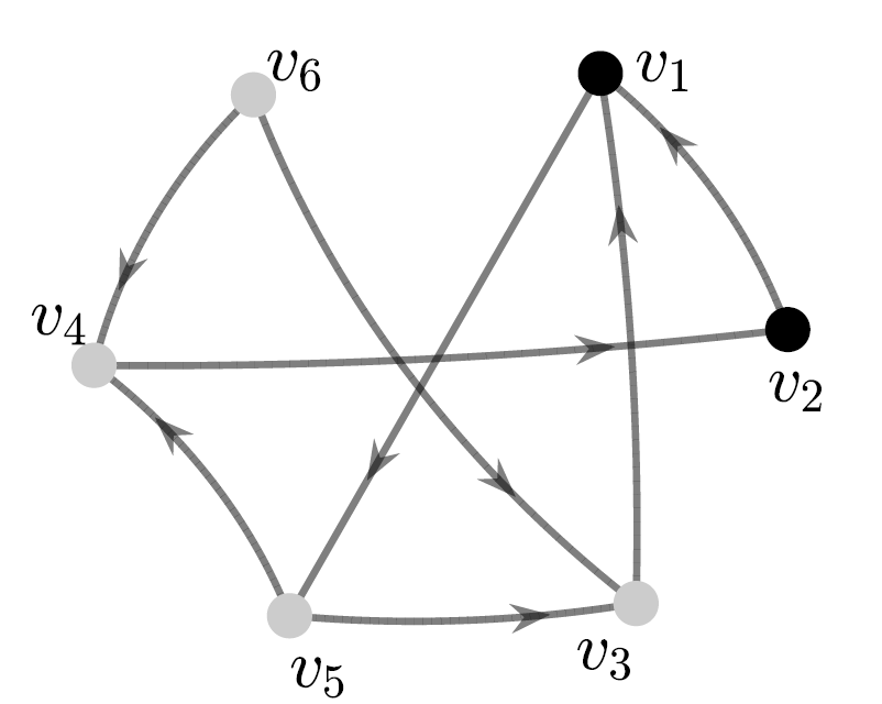
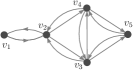
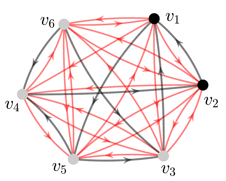
As an example, consider in Figure 1, where is the set of input nodes. As a result of ZF process, infects , infects and the resulting derived set is .
In the context of SSC, the cardinality of the derived set is significant as it provides a lower bound on the dimension of SSCS, as stated in the following result.
Theorem 3.1
[6] For any network with the leaders ,
| (7) |
where is the size of the derived set corresponding to the input set .
III-B Edge Augmentation Algorithm Using ZF
We provide an algorithm to add edges to a directed graph with a given set of leaders. The algorithm ensures that the derived set of the graph remains the same after adding edges, thus, preserving the ZF-based bound on the dimension of SSCS. The proposed algorithm is a modification of the ZF process. In summary, we look for a BLACK node with a single WHITE in-neighbor, add edges incident to the BLACK node that do not change change the size of the derived set, change the WHITE node’s color, and then repeat the same procedure until there is no BLACK node with a single WHITE in-neighbor. When this process concludes, we add any extra edges that can be added while preserving the derived set. The algorithm is outlined below. We denote the color of the node by COLOR().
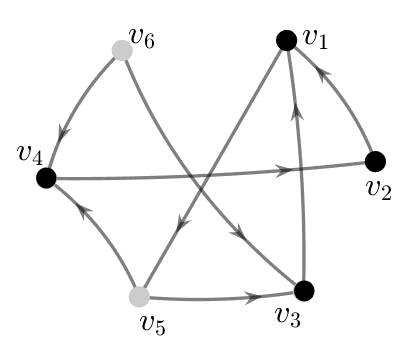
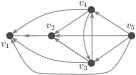
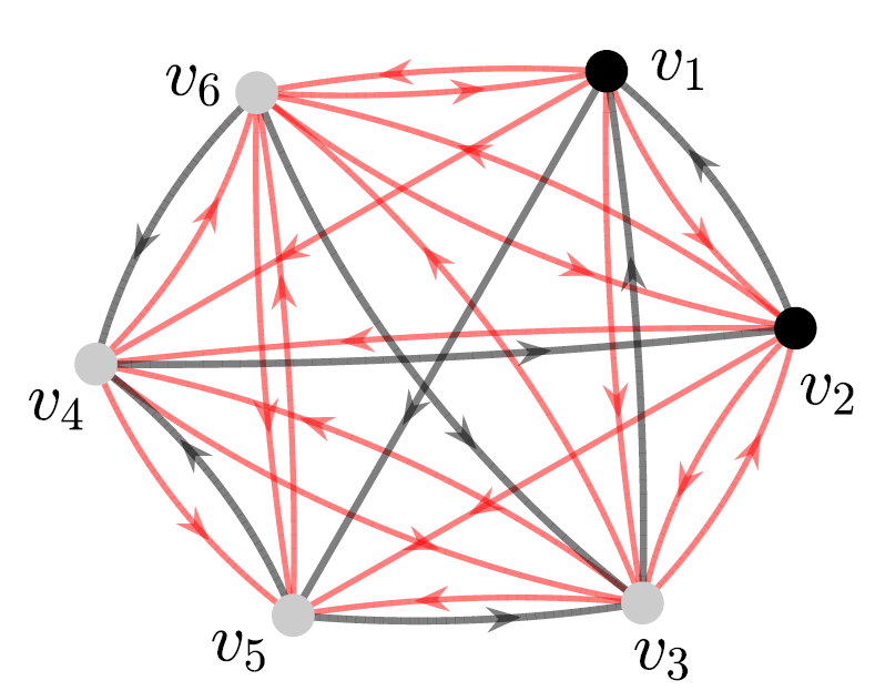
Figure 2(b) illustrates an example of edge augmentation due to Algorithm 1. The derived set in and is same.
.
Next, we show that Algorithm 1 is optimal and adds the maximum number of edges while preserving the size of the derived set returned by the ZF process.
Proposition 3.2
For a directed graph with a leader set , let be a graph returned by Algorithm 1. Then, .
Proof:
Let be the derived set of with a leader set . In , all leader nodes in are colored BLACK due to the initial condition of the ZF process. Consider an arbitrary iteration in the ZF process, where a BLACK node colors its only WHITE in-neighbor BLACK. Algorithm 1 adds edges in from (currently) BLACK nodes to . Since no edge from a currently WHITE node to is added, must be the only WHITE in-neighbor of in as well. Thus, the ZF process proceeds by assigning the BLACK color to node , which is the only WHITE in-neighbor of the BLACK node in . This holds for every iteration in the ZF process. Thus, the ZF process in and will change the colors of nodes exactly the same way.
We can count the number of edges in the directed graph returned by Algorithm 1 in terms of , and the size of the derived set.
Proposition 3.3
Proof:
In each iteration of the WHILE loop in Algorithm 1, edges from all BLACK nodes to a fixed node are added. There are BLACK nodes when the WHILE loop starts, and this number increases by one in each iteration. Thus, we add edges in the WHILE loop. Outside the loop, we add incoming edges for each of the remaining nodes. Therefore,
Theorem 3.4
Let be a directed graph with nodes, leader set and derived set , then Algorithm 1 returns a graph where and is maximum while preserving the size of the derived set . Moreover, the number of edges in the optimal graph is
where
Proof:
Let be a graph satisfying the conditions stated in the theorem, and be a graph returned by Algorithm 1. We will count the number of edges in and show that is upper bound by the expression in Proposition 3.3. Clearly can not be larger than , we will get the desired result.
Since preserves the size of the derived set, we should be able to run iterations of the ZF process in some arbitrary order. When the ZF process starts, there are BLACK nodes and WHITE nodes. At this point, there must exist a BLACK node which has only one in-coming edge from a WHITE in-neighbor. Therefore, at least edges of the form , where is a WHITE node, are missing from . In each iteration, the number of WHITE nodes decreases by exactly one. This means that in the second iteration, at least edges are missing, and these edges are distinct from previously counted edges because none of these involve the node . Similarly, in iteration , there are at least distinct edges missing. We can upper bound the number of edges in by subtarting the minimum number of missing edges in the graph from the maximum possible edges. Thus,
Using Proposition 3.3, we get . However, is optimal, which means . Thus, we deduce that and conclude the desired statement.
The time complexity of Algorithm 1 is where is the number of nodes in the graph. Note that the main task in the algorithm is the addition of edges to the edge set . If the edges are kept in an adjacency matrix, each addition takes a constant amount of time. We do not add an edge twice to this set, so the time complexity is bounded by the maximum number of possible edges in a directed graph. We also observe that the time complexity is:
When the size of derived set is at least , the first term is , and when it is less than , the second term is . Thus, the time complexity of Algorithm 1 is .
Remark 3.5
An important observation here is that the number of edges that one can add to a directed graph while preserving the derived set is independent of the topology of the given graph. Note, however, that the size of the derived set in an arbitrary graph is not independent of the topology.
IV Adding Edges through Distance-based Bound
In this section, first, we review a tight lower bound on the dimension SSCS based on the distances of nodes to leaders in a graph [9]. Second, we present a method to add edges while preserving distances between specific node pairs, which also preserves the bound on the dimension of SSCS. The distance-based bound on the dimension of SSCS is typically better than the ZF-based bound, especially when the network is not strong structurally controllable [10].
IV-A Distance-based Bound for SSC
Given a network with leaders , we define the distance-to-leaders (DL) vector of each as
The component of , denoted by , is equal to the distance of to . Next, we provide the definition of pseudo-monotonically increasing sequences of DL vectors.
-
Definition
(Pseudo-monotonically Increasing (PMI) Sequence) A sequence of distance-to-leaders vectors is PMI if for every vector in the sequence, denoted by , there exists some such that
(8) In other words, (8) needs to be satisfied for all the subsequent distance-to-leader vectors appearing after in the sequence. We say that satisfies the PMI property at coordinate whenever .
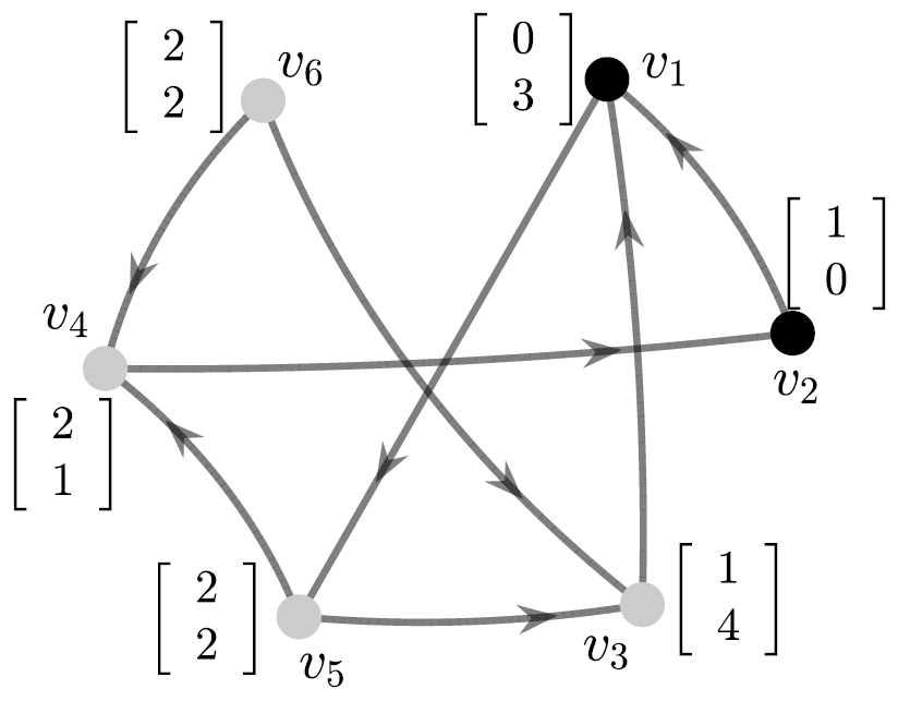
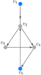
An example of DL vectors is illustrated in Fig. 3. A PMI sequence of length five can be constructed as
| (9) |
Indices of bold values in (9) are the coordinates, , at which the corresponding distance-to-leaders vectors are satisfying the PMI property.
The longest PMI sequence of DL vectors is related to the dimension of SSCS as stated in the following result.
Theorem 4.1
[9] Consider any network with the leaders . Let be the length of the longest PMI sequence of distance-to-leaders vectors with at least one finite entry. Then, .
Remark 4.2
While the bound in Theorem 4.1 was presented for connected undirected graphs in [9, Theorem 3.2], it also holds for any choice of leaders on strongly connected directed graphs as shown in [9, Remark 3.1]. Such connectivity properties already ensure that all DL vectors have only finite entries. The bound can be extended easily to directed graphs without strong connectivity by excluding the DL vectors with all entries.
IV-B Adding Edges While Preserving Node Distances
Let be a graph with a leader set , be a PMI sequence of length , and be the set of nodes whose DL vectors are included in . If we add edges in to obtain a new graph such that the DL vectors of nodes in remain the same in , then will also be a PMI sequence of and . Therefore, one approach to augment edges in a graph while preserving a bound on the dimension of SSCS is to ensure that the distances from a certain set of nodes to leaders do not change due to edge additions. In this direction, we first need to study the maximal edge augmentation in a graph while preserving the distance from a given node to another node .
-
Definition
(Distance Preserving Edge Augmentation (DPEA) Problem) Given a directed graph and nodes such that , find a graph with the (same) node set and an edge set such that and is maximized.
Next, we characterize optimal solutions of the DPEA problem for a given node pair in . We show that the optimal solution belongs to a special class of graphs, which is obtained by the union of clique chains and modified clique chains described below.
-
Definition
(Directed clique chain) A directed graph is a directed clique chain if the node set can be partitioned into sets , such that there is an edge from every node in to every node in for all . Moreover, nodes in each of and induce cliques.222In a clique, there is an edge between every pair of nodes.
-
Definition
(Directed modified clique chain) A directed graph is a directed modified clique chain if the node set can be partitioned into sets , such that there is an edge from every node in to every node in for all .
Examples of directed clique chain and directed modified clique chain are shown in Figure 4.
Theorem 4.3
Let be a directed graph and let be two fixed vertices in with . Then, an augmented graph , that preserves the distance from to , and contains the maximum number of edges is a union of a directed clique chain and a directed modified clique chain for some partition of the node set .
Proof:
Let . Then, it is clear that for all vertices , because otherwise we can add an edge from an arbitrary node at distance to . Also, an arbitrary vertex in at distance from , we may assume that . Clearly, can not be less than , and if it is more, we can add an edge from to a vertex where . Thus, every vertex in lies on a shortest path from to . Let be two vertices such that , and . We have the following cases:
-
1.
or : an edge from to doesn’t change the distance from to . Thus, we may assume that all such edges exist in .
-
2.
: since both of lie on a shortest path from to , we know that . So an edge will create a path from to of distance . This is a contradiction to the fact that preserves distance. Therefore, doesn’t contain any edge of the form .
-
3.
: in this case, an edge from to doesn’t create any new shortest paths from to . Thus, we may assume that all such edges exist in .
Let us define a partition of where . It is clear that with this partition, the graph is a union of a directed clique chain and a directed modified clique chain. This provides a complete characterization of edges in and completes the proof.
From Theorem 4.3, we obtain a simple way to greedily construct a maximally dense graph that preserves the distance from node to node in a given graph as follows:
An example of the DPEA is shown in Figure 5 in which edges are augmented to preserve the distance from node to node .
We note that the time complexity of Algorithm 2 is because we can implement this using runs of Dijkstra’s shortest path algorithm. We can use DPEA to add edges in a graph with a leader set while preserving a bound on the dimension of SSCS. Let be a PMI sequence of length and be the set of nodes whose DL vectors are included in . By solving the DPEA problem for the node pair , where and , we can obtain edges, say , whose addition to the graph will preserve the distance from node to leader . By solving DPEA problem for all node pairs , where and , we can obtain edges that are common in all solutions, that is, . By adding these common edges in the given graph , we obtain a new graph such that , and . Consequently, will also be PMI sequence of , which means that the dimension of SSCS in the augmented graph will also be at least . Thus, by solving multiple instances of DPEA problem, we can determine edges whose addition to the graph will preserve the distance-based bound on the dimension of SSCS.
Since the problem of finding an optimal set of edges while preserving the distance-based bound is computationally challenging, in the next subsection, we present and analyze a randomized edge augmentation algorithm that is simple to understand, easy to implement, and offers good numerical results in our experiments.
IV-C Randomized Edge Augmentation Algorithm Preserving the Distance-based Bound
First, we discuss that for a given , if is a PMI sequence of length containing DL vectors of nodes , then we can add edges in to obtain an augmented graph with the same leader set . Moreover will also have a PMI sequence of length even if , . In particular, for every node pair , where , , there exists an integer such that if , then will have a PMI sequence consisting of DL vectors of nodes in and having a length . We will then provide a randomized edge augmentation algorithm satisfying conditions to preserve the distance-based bound on the dimension of SSCS. Finally, we will analyze the performance of the algorithm.
Let be the vector in the PMI sequence of the given graph . Then by the definition of PMI sequence, for each element , there is an integer, say , such that . We denote the maximum possible value of by and define . For instance, consider the PMI sequence in (9). The vectors in the sequence and the corresponding are given below.
We can think of as a strict lower bound on . From a given PMI sequence of length , we can always obtain for all .
Observation 4.4
In a PMI sequence , if we replace by some integer , where , then the resulting sequence will still be a PMI sequence.
For instance, consider the sequence below, which is obtained from in (9) by replacing and by and , respectively. Since and , the resulting sequence is a PMI sequence.
| (10) |
Next, we present a randomized algorithm to add edges in a graph with a leader set . has a PMI sequence of length consisting of DL vectors of nodes . Moreover, let , where is the index of the node whose DL vector is the element (vector) in . For instance, in (9) is a PMI sequence of the graph in Figure 3. The corresponding is and is . For every vector in the sequence, the algorithm first computes the corresponding vector , which basically provides minimum distances that need to be maintained from node to all leaders during the edge augmentation. The algorithm then selects a missing edge randomly and augments it to the graph if its addition does not violate distance conditions (line 8 in Algorithm 3), otherwise discards it. This process is repeated until all missing edges from the original graph are either added to the graph, or discarded. The details are outlined in Algorithm 3.
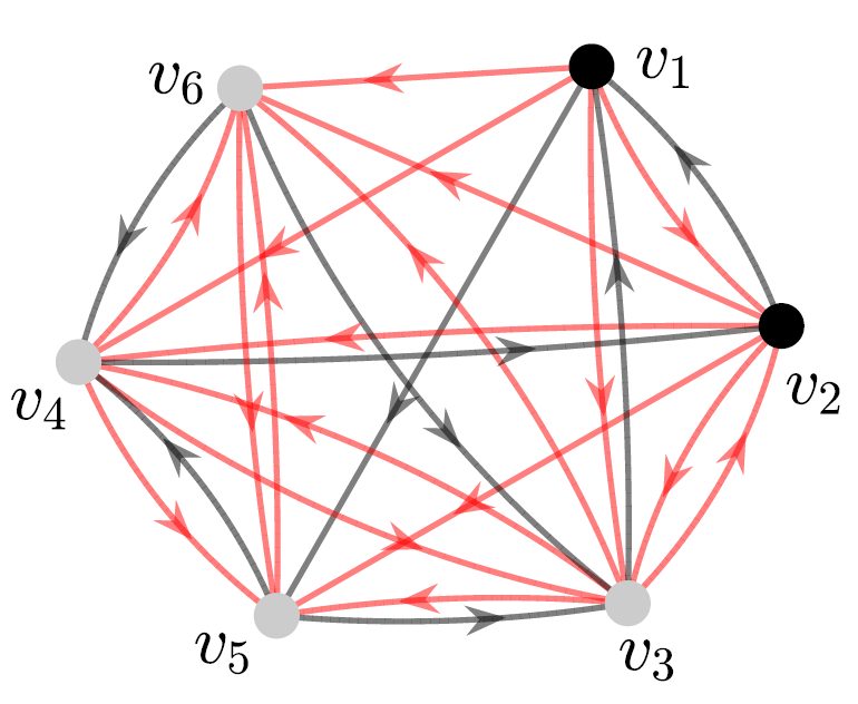
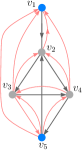
Figure 6(a) illustrates an example of edge augmentation due to Algorithm 3 with the graph in Figure 3 and a PMI sequence of length as inputs. The red edges indicate the augmented edges. We observe that the graph in Figure 6(a) contains a total of 29 edges compared to the graph in Figure 2(b)(b), which contains a total of 25 edges after the ZF-based edge augmentation.
Remark 4.5
We note that the distance-based bound on the dimension of SSCS is typically better than the ZF-based bound, especially when the graph is not SSC [10]. Thus, edge augmentation using Algorithm 3 allows to add edges while preserving a better bound on the dimension of SSCS. For instance, the distance-based bound on the dimension of SSCS in is 5, which is better than the ZF-based bound. We see that using Algorithm 3, we can have a total of 27 edges in the augmented graph (as illustrated in Figure 6(b)) while maintaining the dimension of SSCS to be 5, which is not possible by the edge augmentation using the ZF-based bound.
Next, we analyze the performance of Algorithm 3 by the following result.
Proposition 4.6
If we repeat Algorithm 3 a constant number of times and then return the best graph among these iterations, then the returned graph is an –approximation with probability at least , where is the optimal number of edges and is the number of edges that can each be added without changing the PMI.
We omit the proof of this proposition, because it follows the same arguments given in [11, Proposition 4.2] for a similar result on the undirected graphs. Moreover, the time complexity of Algorithm 3 is , where is the number of edges not in the input graph. The term is the cost of running Dijkstra’s shortest path algorithm for all leader nodes and we do it for all of the missing edges in the randomized algorithm.
V Numerical Evaluation
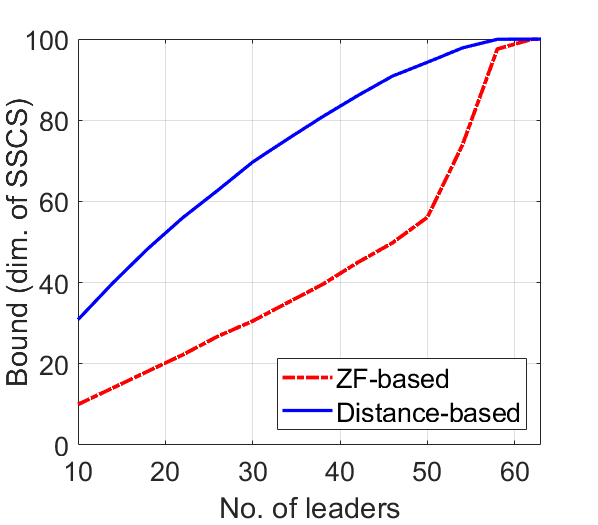
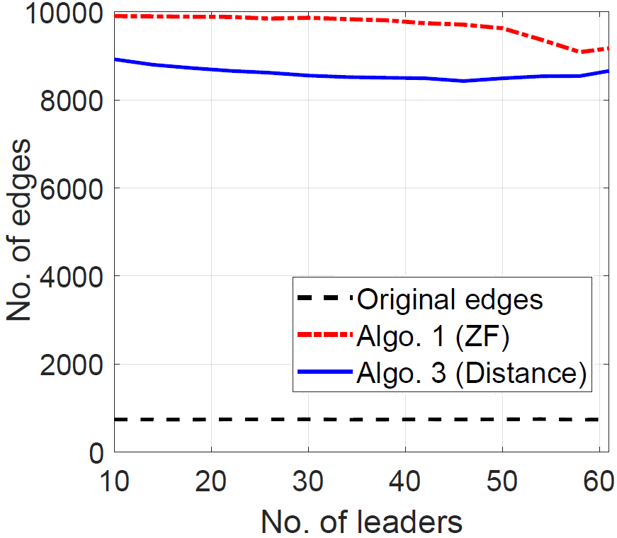
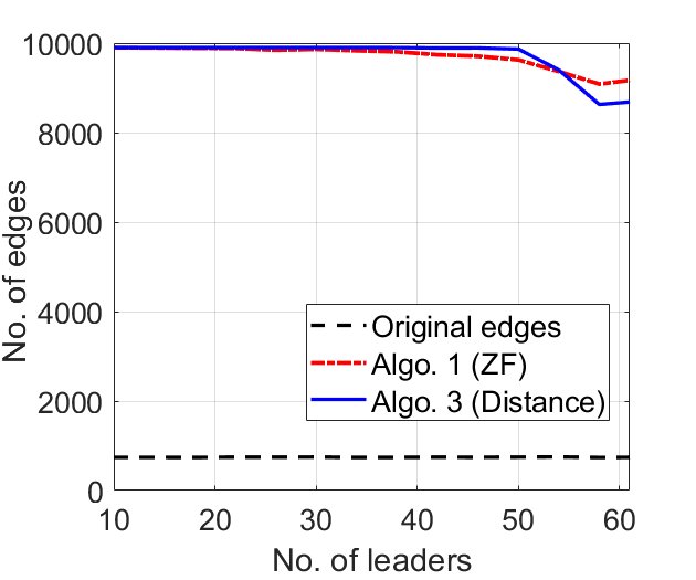
We illustrate and compare the ZF-based and the distance-based edge augmentation algorithms on random directed networks with nodes in which edge exists with probability , . Each point in plots in Figure 7 is an average of 30 randomly generated instances.
In Figure 7(a), we plot ZF-based and distance-based bounds on the dimension of SSCS as a function of number of leaders, which are chosen randomly. The distance-based bound is better than the ZF-based, especially for a smaller number of leaders (as discussed in [10]). Figure 7(b) plots the number of edges added in graphs as a function of number of (randomly selected) leaders. We note that Algorithms 1 and 3 augment edges while preserving the ZF-based and distance-based bounds on the dimension of SSCS, respectively. For the same number of leaders, the number of edges augmented by Algorithm 1 is greater than the Algorithm 3 because the controllability bound preserved by the ZF-based augmentation (Algorithm 1) is smaller than the distance-based augmentation. The number of edges in the original graphs are also shown. Figure 7(c) illustrates the result when we augment edges using Algorithms 1 and 3 while preserving the same controllability bound, which is ZFS-based.
VI Conclusion
Network connectivity and robustness can be improved by augmenting extra links between nodes. However, adding new links may degrade the network’s controllability. In this paper, we presented edge augmentation algorithms to add the maximum number of edges in a network while preserving the ZF-based bound and the distance-based bounds on the dimension of SSCS. When the bound on the dimension of SSCS to be preserved is smaller, a large number of edges can be augmented. Though we considered networks with Laplacian dynamic (2), both the distance-based and the ZF-based methods are applicable to more generalized dynamics in the form (e.g., [12, 5]). In particular, the ZF-based bound holds for any such linear dynamics on a network where an edge denotes that the corresponding entry in the system matrix, , is non-zero. In comparison, the distance-based method requires the system matrix, , to be in a class of matrices called the distance-information-preserving matrices (as explained in [12]), which contain the graph Laplacian as a special case. We aim to further explore the relation between network controllability and edge density to co-optimize robustness and controllability in the future.
References
- [1] W. Abbas, M. Shabbir, Y. Yazıcıoğlu, and A. Akber, “Trade-off between controllability and robustness in diffusively coupled networks,” IEEE Transactions on Control of Network Systems, vol. 7, no. 4, 2020.
- [2] F. Pasqualetti, C. Favaretto, S. Zhao, and S. Zampieri, “Fragility and controllability tradeoff in complex networks,” in American Control Conference (ACC), 2018, pp. 216–221.
- [3] S. S. Mousavi, M. Haeri, and M. Mesbahi, “Strong structural controllability of networks under time-invariant and time-varying topological perturbations,” IEEE Transactions on Automatic Control, 2020.
- [4] G. Lindmark and C. Altafini, “Investigating the effect of edge modifications on networked control systems,” arXiv preprint arXiv:2007.13713, 2020.
- [5] N. Monshizadeh, S. Zhang, and M. K. Camlibel, “Zero forcing sets and controllability of dynamical systems defined on graphs,” IEEE Transactions on Automatic Control, vol. 59, pp. 2562–2567, 2014.
- [6] N. Monshizadeh, K. Camlibel, and H. Trentelman, “Strong targeted controllability of dynamical networks,” in 54th IEEE Conference on Decision and Control (CDC), 2015, pp. 4782–4787.
- [7] M. Trefois and J.-C. Delvenne, “Zero forcing number, constrained matchings and strong structural controllability,” Linear Algebra and its Applications, vol. 484, pp. 199–218, 2015.
- [8] S. S. Mousavi, M. Haeri, and M. Mesbahi, “On the structural and strong structural controllability of undirected networks,” IEEE Transactions on Automatic Control, vol. 63, no. 7, pp. 2234–2241, 2018.
- [9] A. Y. Yazıcıoğlu, W. Abbas, and M. Egerstedt, “Graph distances and controllability of networks,” IEEE Transactions on Automatic Control, vol. 61, no. 12, pp. 4125–4130, 2016.
- [10] A. Y. Yazıcıoğlu, M. Shabbir, W. Abbas, and X. Koutsoukos, “Strong structural controllability of diffusively coupled networks: Comparison of bounds based on distances and Zero Forcing,” in IEEE Conference on Decision and Control (CDC), 2020.
- [11] W. Abbas, M. Shabbir, H. Jaleel, and X. Koutsoukos, “Improving network robustness through edge augmentation while preserving strong structural controllability,” in American Control Conference (ACC), 2020, pp. 2544–2549.
- [12] H. J. Van Waarde, M. K. Camlibel, and H. L. Trentelman, “A distance-based approach to strong target control of dynamical networks,” IEEE Transactions on Automatic Control, vol. 62, no. 12, 2017.
- [13] J. Gao, Y.-Y. Liu, R. M. D’souza, and A.-L. Barabási, “Target control of complex networks,” Nature Communications, vol. 5, 2014.
- [14] A. M. R.-S. G. W. Group, “Zero forcing sets and the minimum rank of graphs,” Linear Algebra and its Applications, vol. 428, no. 7, pp. 1628–1648, 2008.