Edge of Many-Body Quantum Chaos in Quantum Reservoir Computing
Abstract
Reservoir computing (RC) is a machine learning paradigm that harnesses dynamical systems as computational resources. In its quantum extension—quantum reservoir computing (QRC)—these principles are applied to quantum systems, whose rich dynamics broadens the landscape of information processing. In classical RC, optimal performance is typically achieved at the “edge of chaos,” the boundary between order and chaos. Here, we identify its quantum many-body counterpart using the QRC implemented on the celebrated Sachdev-Ye-Kitaev model. Our analysis reveals substantial performance enhancements near two distinct characteristic “edges”: a temporal boundary defined by the Thouless time, beyond which system dynamics is described by random matrix theory, and a parametric boundary governing the transition from integrable to chaotic regimes. These findings establish the “edge of many-body quantum chaos” as a fundamental design principle for QRC.
Introduction. —Quantum mechanics harbors immense potential to revolutionize modern technology [1]. Breakthroughs in quantum computing, communication, and sensing have vividly showcased the transformative power of quantum resources [2, 3, 4, 5]. These advances have, in turn, inspired extensive research efforts in quantum machine learning, with various approaches—notably variational quantum algorithms (VQAs)—being actively explored [6, 7, 8, 9, 10, 11].
More recently, the power of quantum has also integrated with reservoir computing (RC), a machine learning framework renowned for its efficacy in time-series analysis [12, 13, 14, 15, 16]. True to its name, the most distinctive feature of RC is the use of an input-driven dynamical system, known as a “reservoir”, to nonlinearly map input data onto a feature space. Notably, training in RC is limited to the post-processing stage, and the reservoir itself remains fixed. Extending this idea into the quantum domain, Fujii and Nakajima introduced quantum reservoir computing (QRC) [17]. QRC harnesses natural quantum dynamics as a reservoir, generating rich, nonlinear mappings in an exponentially large Hilbert space without encountering the trainability bottlenecks prevalent in VQAs. This capability has sparked significant theoretical progress [18, 19, 20, 21, 22, 23, 24, 25, 26, 27, 28, 29, 30, 31, 32, 33, 34, 35, 36], as well as promising experimental demonstrations [37, 38, 39, 40, 41, 42, 43, 44].
Given the optimization-free nature of RC, researchers naturally ask: What characterizes an effective reservoir system? While this question remains largely unanswered for QRC, several key criteria have been identified for classical RC. The most renowned among them is the concept of the “edge of chaos” [45, 46, 47, 48, 49]. This principle posits that the boundary between chaotic and nonchaotic dynamical regimes provides a performance sweet spot for RC systems, as empirically verified across diverse platforms [50, 51, 52]. By analogy, exploring a quantum version of the edge of chaos offers a promising route to addressing the fundamental question posed above.
In classical systems, chaos is naturally framed via phase space trajectories [53]. In quantum mechanics, however, the Heisenberg uncertainty principle precludes such a direct picture, and one must instead rely on more subtle diagnostics. Early investigations of quantum chaos therefore focused on single-particle systems whose classical limits are chaotic, leading to the conjecture (with some analytical supports) that their spectral statistics are governed by random matrix theory (RMT) [54, 55, 56, 57, 58]. In recent years, attention has shifted to many-body settings, spurred in large part by the exactly solvable Sachdev-Ye-Kitaev (SYK) model [59, 60, 61, 62]. Various diagnostics, including level statistics [63, 64, 65, 66], out-of-time-order correlators [67, 68, 69], and spectral form factors [70, 71, 72, 73] have enriched our understanding of chaos in interacting quantum systems. Experimental realizations of the SYK physics have also been proposed on several platforms [74, 75, 76, 77, 78]. Notably, the SYK model exhibits maximally quantum chaotic behavior, saturating the so-called bound on chaos [79, 69, 80], and has thus stood as a canonical model for the investigation of many-body quantum chaos. These insights motivate the exploration of QRC built upon the SYK model, aiming to address the open question of reservoir effectiveness from a quantum chaotic standpoint.
In this Letter, we explicitly demonstrate key characteristics of effective quantum reservoir systems. In particular, we examine the QRC performance near two distinct chaotic boundaries of the SYK model. The first is a temporal boundary defined by the Thouless time, beyond which the system’s dynamics conforms to RMT. The second is a parametric boundary marking the transition from quantum chaotic to integrable (nonchaotic) behavior, controlled by the strength of an additional noninteracting term. Using representative machine learning tasks that demand both memory retention and nonlinear transformation, we demonstrate that QRC performance is maximized near the onset of quantum chaotic regime in both temporal and parametric domains. These observations establish the “edge of many-body quantum chaos” as a foundational design principle for QRC systems.
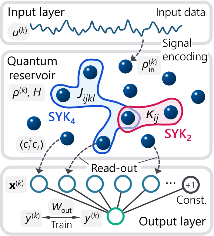
Model. —Figure 1 schematically illustrates the QRC architecture implemented with the SYK model for fermions. The quantum reservoir system, whose dynamics is harnessed for information processing, is governed by the Hamiltonian
| (1) |
where denotes the system size, and () is the spinless fermionic creation (annihilation) operator at site . These operators satisfy the anticommutation relations and . In Eq. (1), the first term describes the SYK4 interaction: the all-to-all couplings are drawn from a zero-mean complex Gaussian distribution of variance ( denotes the ensemble average). The second term is the noninteracting SYK2 contribution, with coupling constants sampled from a zero-mean complex Gaussian distribution of variance . The couplings satisfy the symmetry relations , , and . Both coupling terms conserve the total fermion number . Unless otherwise specified, we set , , and (note that the QRC input protocol introduced below does not conserve ).
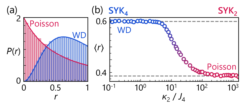
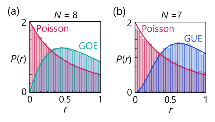
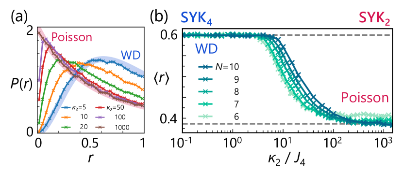
To diagnose the chaotic nature of quantum many-body systems, we first examine the level statistics [63, 64, 65, 66]. Let the ordered eigenvalues of be ; the spacings between consecutive energy levels are given by . In an integrable system, the spacing distribution follows Poisson statistics, whereas in a quantum chaotic system, it is well described by Wigner-Dyson (WD) distribution. A convenient metric to characterize these distributions is the level spacing ratio, defined as . Its mean value assumes for Poisson distribution and for WD statistics [63, 64]. Figure 2(a) presents the distribution of the level spacing ratio for the SYK4 model [] and the SYK2 model [], in excellent agreement with the WD and Poisson predictions, respectively. Notably, when both terms are present, the system can be tuned between these extremes: as the ratio of the typical coupling strengths increases, Fig. 2(b) displays a gradual shift of from the WD to the Poisson value. Despite the smearing effects associated with finite system sizes, this result strongly suggests the emergence of the quantum chaotic to integrable transition [81, 82, 83, 84, 85] (see the Supplemental Material [86]).
Framework of the QRC. —We now describe the QRC framework for information processing; all procedures employed herein follow the conventional protocols established in earlier investigations [17, 18]. The QRC architecture comprises four principal stages: signal encoding, reservoir dynamics, read-out, and post-processing, through which the input at the -th step is processed in an attempt to produce its corresponding target value (Fig. 1). Consider a discretized input sequence with . Each input is encoded into the reservoir by replacing the quantum state at site with , where . Subsequently, the system evolves unitarily under the Hamiltonian in Eq. (1). The encoding operation is repeated at intervals , which determines the intrinsic time-scale of the QRC system. The overall update rule is summarized by the completely positive trace-preserving map:
| (2) |
where denotes the partial trace over site ; see the Supplemental Material [86] for details on the observed dynamics. During the evolution, the expectation value of the single-site particle number is measured at discrete times , where and is the number of virtual computational nodes (here, ). At the -th step, the outcomes are assembled into a one-dimensional state vector ; including an additional constant term, has components in total. The output layer then applies a linear transformation , where the output weight is trained by minimizing the mean squared error between the computed output and the target output . In our simulations, a total of inputs are processed. Starting from a random initial state, the first inputs are discarded to wash out the effects of initial conditions; for the convergence property, see the Supplemental Material [86]. The subsequent inputs are employed for training , and the final are reserved for evaluation. Performance results are averaged over independent random realizations.
We evaluate the reservoir performance on two complementary tasks: the short-term memory (STM) task, which probes linear memory capacity, and the nonlinear auto-regressive moving average (NARMA) task, which evaluates combined memory and nonlinear processing capabilities [14, 17].
In the STM task, the target output at delay is defined as the input value steps earlier in a random input sequence , i.e., . During the testing phase, we collect the outputs and targets , and compute the determination coefficient , where and denote the covariance and the variance, respectively. is bounded between and ; values closer to indicate better memory performance.
In the NARMA task, the target sequence at a given order is defined by the recursive relation: , where (, , , ) are set to (, , , ) [17, 20]. The input stream is sampled from the range to prevent divergence in , which is then rescaled to when encoded to the quantum reservoir [17]. Performance is evaluated in terms of the deviation between the output and the target, which is quantified by the normalized mean-squared error (NMSE) with being the Euclidean norm. A lower NMSE indicates superior performance in accurately reproducing the target nonlinear dynamics.
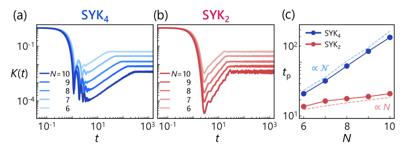
Temporal edge of many-body quantum chaos. —Our investigation begins with an examination of the QRC performance of the SYK4 and SYK2 models, in which clear fingerprints of many-body quantum chaos manifest themselves in the temporal domain. As a time-domain probe of the energy-spectrum correlations characteristic of quantum chaos, we analyze the spectral form factor (SFF) , where denotes the Hilbert space dimension [70, 71, 72, 73]. In many-body chaotic systems, the SFF generally exhibits a “ramp-plateau” profile governed by two time-scales: the Thouless time , after which the evolution shows a universal “ramp” and follows RMT predictions, and the plateau time , beyond which saturates at a plateau. Figures 3(a) and 3(b) illustrate the SFF for the SYK4 and SYK2 limits, respectively. Notably, in the SYK4 case, the SFF exhibits the pronounced ramp beginning around and the subsequent plateau beyond , providing a clear signature of many-body quantum chaos. While in the SYK2 model also features a dip and a plateau, they occur on a much shorter timescale and with a different system-size scaling of compared to the chaotic system (see the Supplemental Material for details [86]).
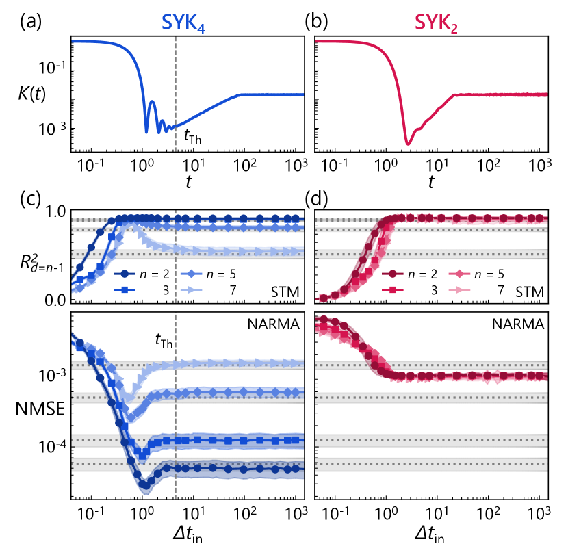
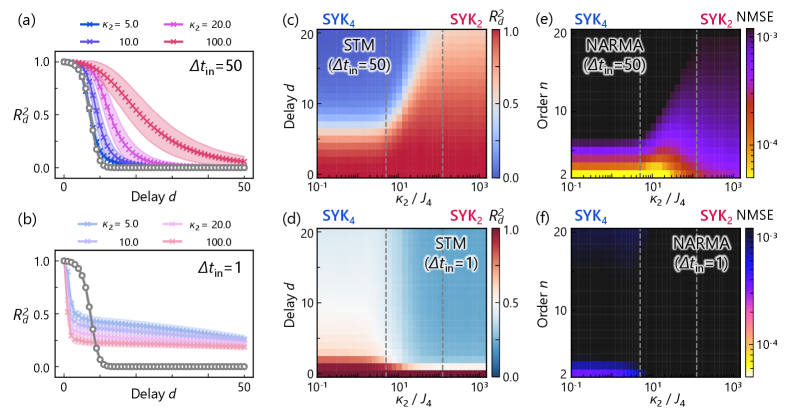
Turning to computational benchmarks, Figs. 3(c) and 3(d) plot the QRC performance of the SYK4 and SYK2 models as functions of the input interval , which defines the intrinsic time-scale governing the QRC dynamics. The upper panels display the STM performance at delay , and the lower panels show the NMSE on the NARMA- tasks of orders , , , and . The chosen STM delay corresponds to the oldest input term explicitly appearing in the recursive definition of the NARMA- dynamics; additional past inputs are nevertheless implicitly encoded within the target sequence (see the Supplemental Material for the full delay dependence of [86]). To establish a baseline for comparison, we also analyze the Haar QRC model, in which the evolution operator is replaced by a unitary drawn from the Haar measure [87, 88]. Its performance, shown as horizontal dashed lines, deteriorates monotonically with increasing as the task complexity grows.
A striking pattern emerges in the QRC performance for the SYK4 model [Fig. 3(c)]. When is very small, the time evolution of the quantum reservoir does not yield an effective feature map, resulting in poor performance on both the STM and NARMA tasks. However, as increases toward the Thouless time , the QRC performance improves dramatically and reaches its maximum just before . Beyond this point, both metrics level off at the baseline of the Haar QRC model for each order , in accordance with the onset of universal RMT descriptions typical of quantum chaotic systems. In other words, the Thouless time effectively marks the temporal boundary where fully quantum chaotic signatures begin to dominate the QRC performance. The observed peak, situated just prior to , thus explicitly underscores the performance enhancement at the “edge of many-body quantum chaos” in the temporal domain.
In contrast, the QRC with the integrable SYK2 model behaves quite differently [Fig. 3(d)]. As increases, the NARMA performance improves only modestly from its initial low values and quickly saturates. No pronounced performance peak emerges therein. This behavior starkly contrasts with that of the SYK4 model, indicating that the performance enhancements observed in Fig. 3(c) are fundamentally attributable to the latter’s intrinsic many-body quantum chaotic nature. Notably, despite its poor NARMA performance, the STM metric for the SYK2 model remains close to for sufficiently large values of , surpassing both the SYK4 model and the Haar QRC reference. This exemplifies the well-established trade-off in RC between memory capacity and nonlinear transformation capability [89, 90, 91]: QRC with the integrable SYK2 model retains strong memory but lacks nonlinear richness required for complex tasks. These model-dependent behaviors motivate our exploration of interpolations between the SYK2 and SYK4 models.
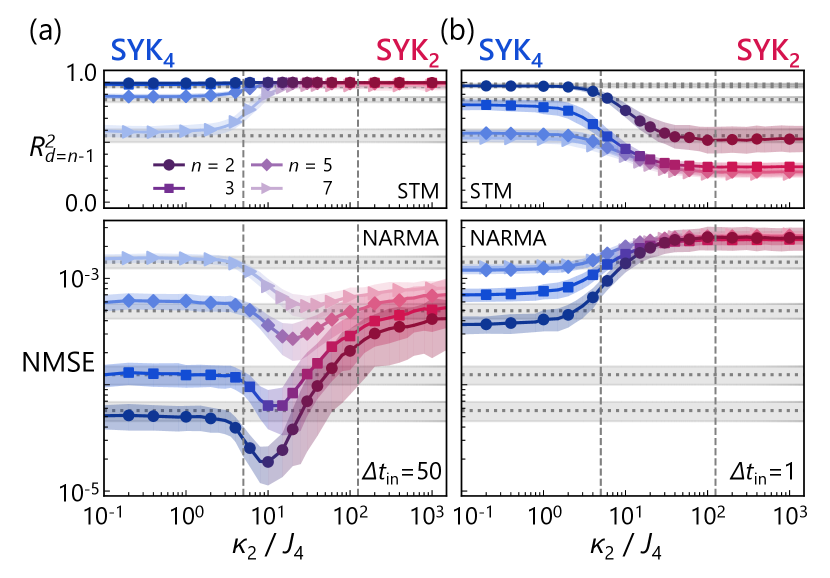
Parametric edge of many-body quantum chaos. —We here demonstrate the QRC performance across the chaotic-integrable transition by mixing the SYK4 and SYK2 Hamiltonians. To ensure a fair comparison as the coupling strength is varied, each Hamiltonian is rescaled by its spectral norm: [92]. (Note that this correspondingly changes the time-scale relative to Fig. 3.) Figures 4(a) and 4(b) display the STM and NARMA performances versus the ratio for long () and short () input intervals, respectively. The vertical dashed lines serve as a guide of the eye for the onset of WD and Poisson statistics, while the horizontal dotted lines represent the performance of the Haar QRC model for reference. We note that these input intervals are chosen to probe two distinct time-scales: the longer input interval evaluates QRC performance within the universal RMT regime, while the shorter interval characterizes QRC behavior in the nonuniversal, short-time window outside the scope of RMT (see the Supplemental Material [86]).
The most pronounced trend is observed for [Fig. 4(a)]. When is varied, the NARMA performance exhibits a clear peak at a coupling strength just before the onset of the many-body quantum chaotic regime. This peak provides another manifestation of the “edge of many-body quantum chaos”, in this case in the parameter domain. By contrast, for the short input interval , varying the coupling strength yields no performance enhancement [Fig. 4(b)]. At such a short time-scale, the QRC does not reflect chaotic characteristics, so the performance changes only gradually, without any distinct peak at the chaos boundary.
We remark that the specifics of performance enhancement are task-dependent. For instance, in the higher-order tasks detailed in the Supplementary Material, both the position and strength of performance peaks vary with the order [86]. Nevertheless, the fundamental trend remains robust: the most pronounced improvements appear at the edge of many-body quantum chaos. Moreover, since the NARMA task captures nonlinear temporal dynamics that mirror those in real-world systems, the performance boosts shown on this task strongly suggest that similar improvements will extend to a broad class of practical temporal processing applications.
Discussions. —Recent advances in QRC have yielded related performance enhancements, and we believe that a concise comparison highlights the significance of our contributions. One of the authors and his collaborators identified a performance peak near the operational regime boundary in their feedback-driven QRC protocol [32]; however, this enhancement appears predominantly due to classical instabilities in feedback connections, rather than intrinsically quantum phenomena. In the purely quantum regime, Martínez-Peña et al. demonstrated enhanced performance near the ergodic-localization transition in the spin-based QRC [20, 23, 33]. While this finding highlights the importance of dynamical phases in QRC, the role of many-body quantum chaos, and its relation to RMT, remain largely unexplored. Recently, Llodrà et al. analyzed QRC performance in connection with quantum chaos at the quantum phase transition between superfluid and Mott insulator in a clean system, which is complementary to our study on random systems [34]. From a standpoint of temporal domain, investigations into quantum chaos remain sparse: Vetrano et al. explored the role of scrambling times, though within a different framework (quantum extreme learning machines) that does not consider memory of sequential inputs [88].
Building upon these studies, our work clarifies the key characteristics that endow QRC with high computational performance. We have extended the concept of the “edge of chaos” into the quantum realm, investigating how many-body quantum chaos influences QRC in both temporal and parametric domains. The SYK model—a canonical many-body quantum chaotic system—serves as an ideal testbed. Through a unified analysis, we have revealed two distinct optimal regimes: one is the “temporal edge”, which emerges before the Thouless time, and the other is the “parametric edge”, which appears near the quantum chaotic-to-integrable transition. These findings integrate existing knowledge and establish a general principle: optimal QRC performance occurs at the “edge of many-body quantum chaos”. Our study therefore provides clear design principles for engineering quantum reservoirs, unlocking advanced information processing with quantum many-body systems.
Acknowledgments. —The authors thank Shusei Wadashima for fruitful discussions. This work was supported by the JSPS KAKENHI (No. JP25H01247). K.K. was supported by the Program for Leading Graduate Schools (MERIT-WINGS) and JST BOOST (No. JPMJBS2418). Part of computation in this work has been done using the facilities of the Supercomputer Center, the Institute for Solid State Physics, the University of Tokyo.
References
- Feynman [1982] R. P. Feynman, Simulating physics with computers, Int. J. Theor. Phys. 21, 467 (1982).
- Arute et al. [2019] F. Arute, K. Arya, R. Babbush, D. Bacon, J. C. Bardin, R. Barends, R. Biswas, S. Boixo, F. G. S. L. Brandao, D. A. Buell, et al., Quantum supremacy using a programmable superconducting processor, Nature 574, 505 (2019).
- Zhong et al. [2020] H.-S. Zhong, H. Wang, Y.-H. Deng, M.-C. Chen, L.-C. Peng, Y.-H. Luo, J. Qin, D. Wu, X. Ding, Y. Hu, et al., Quantum computational advantage using photons, Science 370, 1460 (2020).
- Gisin et al. [2002] N. Gisin, G. Ribordy, W. Tittel, and H. Zbinden, Quantum cryptography, Rev. Mod. Phys. 74, 145 (2002).
- Degen et al. [2017] C. L. Degen, F. Reinhard, and P. Cappellaro, Quantum sensing, Rev. Mod. Phys. 89, 035002 (2017).
- Peruzzo et al. [2014] A. Peruzzo, J. McClean, P. Shadbolt, M.-H. Yung, X.-Q. Zhou, P. J. Love, A. Aspuru-Guzik, and J. L. O’Brien, A variational eigenvalue solver on a photonic quantum processor, Nat. Commun. 5, 4213 (2014).
- Biamonte et al. [2017] J. Biamonte, P. Wittek, N. Pancotti, P. Rebentrost, N. Wiebe, and S. Lloyd, Quantum machine learning, Nature 549, 195 (2017).
- McClean et al. [2018] J. R. McClean, S. Boixo, V. N. Smelyanskiy, R. Babbush, and H. Neven, Barren plateaus in quantum neural network training landscapes, Nat. Commun. 9, 4812 (2018).
- Mitarai et al. [2018] K. Mitarai, M. Negoro, M. Kitagawa, and K. Fujii, Quantum circuit learning, Phys. Rev. A 98, 032309 (2018).
- HavlÃÄek et al. [2019] V. HavlÃÄek, A. D. Córcoles, K. Temme, A. W. Harrow, A. Kandala, J. M. Chow, and J. M. Gambetta, Supervised learning with quantum-enhanced feature spaces, Nature 567, 209 (2019).
- Cerezo et al. [2021] M. Cerezo, A. Arrasmith, R. Babbush, S. C. Benjamin, S. Endo, K. Fujii, J. R. McClean, K. Mitarai, X. Yuan, L. Cincio, and P. J. Coles, Variational quantum algorithms, Nat. Rev. Phys. 3, 625 (2021).
- Jaeger [2001] H. Jaeger, The “echo state” approach to analysing and training recurrent neural networks-with an erratum note, Bonn, Germany: German National Research Center for Information Technology GMD Technical Report 148, 13 (2001).
- Jaeger and Haas [2004] H. Jaeger and H. Haas, Harnessing nonlinearity: Predicting chaotic systems and saving energy in wireless communication, Science 304, 78 (2004).
- Verstraeten et al. [2007] D. Verstraeten, B. Schrauwen, M. D’Haene, and D. Stroobandt, An experimental unification of reservoir computing methods, Neural Netw. 20, 391 (2007).
- Tanaka et al. [2019] G. Tanaka, T. Yamane, J. B. Héroux, R. Nakane, N. Kanazawa, S. Takeda, H. Numata, D. Nakano, and A. Hirose, Recent advances in physical reservoir computing: A review, Neural Netw. 115, 100 (2019).
- Kobayashi and Motome [2023] K. Kobayashi and Y. Motome, Thermally-robust spatiotemporal parallel reservoir computing by frequency filtering in frustrated magnets, Sci. Rep. 13, 15123 (2023).
- Fujii and Nakajima [2017] K. Fujii and K. Nakajima, Harnessing disordered-ensemble quantum dynamics for machine learning, Phys. Rev. Appl. 8, 024030 (2017).
- Nakajima et al. [2019] K. Nakajima, K. Fujii, M. Negoro, K. Mitarai, and M. Kitagawa, Boosting computational power through spatial multiplexing in quantum reservoir computing, Phys. Rev. Appl. 11, 034021 (2019).
- Ghosh et al. [2019] S. Ghosh, A. Opala, M. Matuszewski, T. Paterek, and T. C. H. Liew, Quantum reservoir processing, npj Quantum Inf. 5, 35 (2019).
- Martínez-Peña et al. [2021] R. Martínez-Peña, G. L. Giorgi, J. Nokkala, M. C. Soriano, and R. Zambrini, Dynamical Phase Transitions in Quantum Reservoir Computing, Phys. Rev. Lett. 127, 100502 (2021).
- Nokkala et al. [2021] J. Nokkala, R. Martínez-Peña, G. L. Giorgi, V. Parigi, M. C. Soriano, and R. Zambrini, Gaussian states of continuous-variable quantum systems provide universal and versatile reservoir computing, Commun. Phys. 4, 53 (2021).
- Sakurai et al. [2022] A. Sakurai, M. P. Estarellas, W. J. Munro, and K. Nemoto, Quantum extreme reservoir computation utilizing scale-free networks, Phys. Rev. Appl. 17, 064044 (2022).
- Xia et al. [2022] W. Xia, J. Zou, X. Qiu, and X. Li, The reservoir learning power across quantum many-body localization transition, Front. Phys. 17, 33506 (2022).
- Bravo et al. [2022] R. A. Bravo, K. Najafi, X. Gao, and S. F. Yelin, Quantum reservoir computing using arrays of rydberg atoms, PRX Quantum 3, 030325 (2022).
- Martínez-Peña et al. [2023] R. Martínez-Peña, J. Nokkala, G. L. Giorgi, R. Zambrini, and M. C. Soriano, Information Processing Capacity of Spin-Based Quantum Reservoir Computing Systems, Cogn. Comput. 15, 1440 (2023).
- Mujal et al. [2023] P. Mujal, R. Martínez-Peña, G. L. Giorgi, M. C. Soriano, and R. Zambrini, Time-series quantum reservoir computing with weak and projective measurements, npj Quantum Inf. 9, 16 (2023).
- Llodrà et al. [2023] G. Llodrà , C. Charalambous, G. L. Giorgi, and R. Zambrini, Benchmarking the role of particle statistics in quantum reservoir computing, Adv. Quantum Technol. 6, 2200100 (2023).
- Yasuda et al. [2023] T. Yasuda, Y. Suzuki, T. Kubota, K. Nakajima, Q. Gao, W. Zhang, S. Shimono, H. I. Nurdin, and N. Yamamoto, Quantum reservoir computing with repeated measurements on superconducting devices, arXiv preprint arXiv:2310.06706 (2023).
- Sannia et al. [2024] A. Sannia, R. Martínez-Peña, M. C. Soriano, G. L. Giorgi, and R. Zambrini, Dissipation as a resource for Quantum Reservoir Computing, Quantum 8, 1291 (2024).
- Palacios et al. [2024] A. Palacios, R. MartÃnez-Peña, M. C. Soriano, G. L. Giorgi, and R. Zambrini, Role of coherence in many-body Quantum Reservoir Computing, Commun. Phys. 7, 369 (2024).
- Čindrak et al. [2024] S. Čindrak, B. Donvil, K. Lüdge, and L. Jaurigue, Enhancing the performance of quantum reservoir computing and solving the time-complexity problem by artificial memory restriction, Phys. Rev. Res. 6, 013051 (2024).
- Kobayashi et al. [2024] K. Kobayashi, K. Fujii, and N. Yamamoto, Feedback-driven quantum reservoir computing for time-series analysis, PRX Quantum 5, 040325 (2024).
- Ivaki et al. [2024] M. N. Ivaki, A. Lazarides, and T. Ala-Nissila, Quantum reservoir computing on random regular graphs, arXiv preprint arXiv:2409.03665 (2024).
- Llodrà et al. [2025] G. Llodrà , P. Mujal, R. Zambrini, and G. L. Giorgi, Quantum reservoir computing in atomic lattices, Chaos, Solitons & Fractals 195, 116289 (2025).
- Kobayashi and Motome [2025a] K. Kobayashi and Y. Motome, Quantum reservoir probing: An inverse paradigm of quantum reservoir computing for exploring quantum many-body physics, SciPost Phys. 18, 198 (2025a).
- Kobayashi and Motome [2025b] K. Kobayashi and Y. Motome, Quantum reservoir probing of quantum phase transitions, Nat. Commun. 16, 3871 (2025b).
- Negoro et al. [2018] M. Negoro, K. Mitarai, K. Fujii, K. Nakajima, and M. Kitagawa, Machine learning with controllable quantum dynamics of a nuclear spin ensemble in a solid, arXiv preprint arXiv:1806.10910 (2018).
- Chen et al. [2020] J. Chen, H. I. Nurdin, and N. Yamamoto, Temporal information processing on noisy quantum computers, Phys. Rev. Appl. 14, 024065 (2020).
- Suzuki et al. [2022] Y. Suzuki, Q. Gao, K. C. Pradel, K. Yasuoka, and N. Yamamoto, Natural quantum reservoir computing for temporal information processing, Sci. Rep. 12, 1353 (2022).
- Kubota et al. [2023] T. Kubota, Y. Suzuki, S. Kobayashi, Q. H. Tran, N. Yamamoto, and K. Nakajima, Temporal information processing induced by quantum noise, Phys. Rev. Res. 5, 023057 (2023).
- Hu et al. [2023] F. Hu, G. Angelatos, S. A. Khan, M. Vives, E. Türeci, L. Bello, G. E. Rowlands, G. J. Ribeill, and H. E. Türeci, Tackling sampling noise in physical systems for machine learning applications: Fundamental limits and eigentasks, Phys. Rev. X 13, 041020 (2023).
- Senanian et al. [2024] A. Senanian, S. Prabhu, V. Kremenetski, S. Roy, Y. Cao, J. Kline, T. Onodera, L. G. Wright, X. Wu, V. Fatemi, and P. L. McMahon, Microwave signal processing using an analog quantum reservoir computer, Nat. Commun. 15, 7490 (2024).
- KornjaÄa et al. [2024] M. KornjaÄa, H.-Y. Hu, C. Zhao, J. Wurtz, P. Weinberg, M. Hamdan, A. Zhdanov, S. H. Cantu, H. Zhou, R. A. Bravo, et al., Large-scale quantum reservoir learning with an analog quantum computer, arXiv preprint arXiv:2407.02553 (2024).
- Suprano et al. [2024] A. Suprano, D. Zia, L. Innocenti, S. Lorenzo, V. Cimini, T. Giordani, I. Palmisano, E. Polino, N. Spagnolo, F. Sciarrino, G. M. Palma, A. Ferraro, and M. Paternostro, Experimental property reconstruction in a photonic quantum extreme learning machine, Phys. Rev. Lett. 132, 160802 (2024).
- Packard [1988] N. H. Packard, Adaptation toward the edge of chaos, in Dynamic Patterns in Complex Systems, Vol. 212, edited by J. A. S. Kelso, A. J. Mandell, and M. F. Shlesinger (World Scientific, Singapore, 1988) pp. 293–301.
- Langton [1990] C. G. Langton, Computation at the edge of chaos: Phase transitions and emergent computation, Physica D 42, 12 (1990).
- Bertschinger and Natschläger [2004] N. Bertschinger and T. Natschläger, Real-time computation at the edge of chaos in recurrent neural networks, Neural Comput. 16, 1413 (2004).
- Legenstein and Maass [2007] R. Legenstein and W. Maass, Edge of chaos and prediction of computational performance for neural circuit models, Neural Netw. 20, 323 (2007), echo State Networks and Liquid State Machines.
- Boedecker et al. [2012] J. Boedecker, O. Obst, J. T. Lizier, M. M. N, and M. Asada, Information processing in echo state networks at the edge of chaos, Theory Biosci. 131, 205 (2012).
- Takano et al. [2018] K. Takano, C. Sugano, M. Inubushi, K. Yoshimura, S. Sunada, K. Kanno, and A. Uchida, Compact reservoir computing with a photonic integrated circuit, Opt. Express 26, 29424 (2018).
- Hochstetter et al. [2021] J. Hochstetter, R. Zhu, A. Loeffler, A. Diaz-Alvarez, T. Nakayama, and Z. Kuncic, Avalanches and edge-of-chaos learning in neuromorphic nanowire networks, Nat. Commun. 12, 4008 (2021).
- Nishioka et al. [2022] D. Nishioka, T. Tsuchiya, W. Namiki, M. Takayanagi, M. Imura, Y. Koide, T. Higuchi, and K. Terabe, Edge-of-chaos learning achieved by ion-electronâcoupled dynamics in an ion-gating reservoir, Sci. Adv. 8, eade1156 (2022).
- Ott [2002] E. Ott, Chaos in Dynamical Systems, 2nd ed. (Cambridge University Press, 2002).
- Brody et al. [1981] T. A. Brody, J. Flores, J. B. French, P. A. Mello, A. Pandey, and S. S. M. Wong, Random-matrix physics: spectrum and strength fluctuations, Rev. Mod. Phys. 53, 385 (1981).
- Bohigas et al. [1984] O. Bohigas, M. J. Giannoni, and C. Schmit, Characterization of Chaotic Quantum Spectra and Universality of Level Fluctuation Laws, Phys. Rev. Lett. 52, 1 (1984).
- Berry [1985] M. V. Berry, Semiclassical theory of spectral rigidity, Proc. R. Soc. A 400, 229 (1985).
- Guhr et al. [1998] T. Guhr, A. MüllerâGroeling, and H. A. Weidenmüller, Random-matrix theories in quantum physics: common concepts, Phys. Rep. 299, 189 (1998).
- Müller et al. [2004] S. Müller, S. Heusler, P. Braun, F. Haake, and A. Altland, Semiclassical Foundation of Universality in Quantum Chaos, Phys. Rev. Lett. 93, 014103 (2004).
- Sachdev and Ye [1993] S. Sachdev and J. Ye, Gapless spin-fluid ground state in a random quantum heisenberg magnet, Phys. Rev. Lett. 70, 3339 (1993).
- Kitaev [2015] A. Kitaev, Entanglement in strongly correlated quantum matter (2015), https://online.kitp.ucsb.edu/online/entangled15/.
- Sachdev [2015] S. Sachdev, Bekenstein-Hawking Entropy and Strange Metals, Phys. Rev. X 5, 041025 (2015).
- Fu and Sachdev [2016] W. Fu and S. Sachdev, Numerical study of fermion and boson models with infinite-range random interactions, Phys. Rev. B 94, 035135 (2016).
- Oganesyan and Huse [2007] V. Oganesyan and D. A. Huse, Localization of interacting fermions at high temperature, Phys. Rev. B 75, 155111 (2007).
- Atas et al. [2013] Y. Y. Atas, E. Bogomolny, O. Giraud, and G. Roux, Distribution of the Ratio of Consecutive Level Spacings in Random Matrix Ensembles, Phys. Rev. Lett. 110, 084101 (2013).
- Haake et al. [2018] F. Haake, S. Gnutzmann, and M. KuÅ, Quantum Signatures of Chaos, 4th ed., Springer Series in Synergetics (Springer, 2018).
- Giraud et al. [2022] O. Giraud, N. Macé, E. Vernier, and F. Alet, Probing symmetries of quantum many-body systems through gap ratio statistics, Phys. Rev. X 12, 011006 (2022).
- Roberts and Stanford [2015] D. A. Roberts and D. Stanford, Diagnosing Chaos Using Four-Point Functions in Two-Dimensional Conformal Field Theory, Phys. Rev. Lett. 115, 131603 (2015).
- Roberts and Yoshida [2017] D. A. Roberts and B. Yoshida, Chaos and complexity by design, J. High Energ. Phys. 2017, 121.
- Maldacena et al. [2016] J. Maldacena, S. H. Shenker, and D. Stanford, A bound on chaos, J. High Energ. Phys. 2016, 106.
- Cotler et al. [2017a] J. S. Cotler, G. Gur-Ari, M. Hanada, J. Polchinski, P. Saad, S. H. Shenker, D. Stanford, A. Streicher, and M. Tezuka, Black holes and random matrices, J. High Energ. Phys. 2017, 118.
- Cotler et al. [2017b] J. S. Cotler, N. Hunter-Jones, J. Liu, and B. Yoshida, Chaos, complexity, and random matrices, J. High Energ. Phys. 2017, 48.
- Liu [2018] J. Liu, Spectral form factors and late time quantum chaos, Phys. Rev. D 98, 086026 (2018).
- Gharibyan et al. [2018] H. Gharibyan, M. Hanada, S. H. Shenker, and M. Tezuka, Onset of random matrix behavior in scrambling systems, J. High Energ. Phys. 2018 (07).
- Danshita et al. [2017] I. Danshita, M. Hanada, and M. Tezuka, Creating and probing the SachdevâYeâKitaev model with ultracold gases: Towards experimental studies of quantum gravity, Prog. Theor. Exp. Phys. 2017, 083I01 (2017).
- García-Álvarez et al. [2017] L. García-Álvarez, I. L. Egusquiza, L. Lamata, A. del Campo, J. Sonner, and E. Solano, Digital Quantum Simulation of Minimal , Phys. Rev. Lett. 119, 040501 (2017).
- Pikulin and Franz [2017] D. I. Pikulin and M. Franz, Black Hole on a Chip: Proposal for a Physical Realization of the Sachdev-Ye-Kitaev model in a Solid-State System, Phys. Rev. X 7, 031006 (2017).
- Luo et al. [2019] Z. Luo, Y.-Z. You, J. Li, C.-M. Jian, D. Lu, C. Xu, B. Zeng, and R. Laflamme, Quantum simulation of the non-fermi-liquid state of Sachdev-Ye-Kitaev model, npj Quantum Inf. 5, 53 (2019).
- Jafferis et al. [2022] D. Jafferis, A. Zlokapa, J. D. Lykken, D. K. Kolchmeyer, S. I. Davis, N. Lauk, H. Neven, and M. Spiropulu, Traversable wormhole dynamics on a quantum processor, Nature 612, 51 (2022).
- Polchinski and Rosenhaus [2016] J. Polchinski and V. Rosenhaus, The spectrum in the Sachdev-Ye-Kitaev model, J. High Energ. Phys. 2016, 1.
- Maldacena and Stanford [2016] J. Maldacena and D. Stanford, Remarks on the Sachdev-Ye-Kitaev model, Phys. Rev. D 94, 106002 (2016).
- García-García et al. [2018] A. M. García-García, B. Loureiro, A. Romero-Bermúdez, and M. Tezuka, Chaotic-Integrable Transition in the Sachdev-Ye-Kitaev Model, Phys. Rev. Lett. 120, 241603 (2018).
- Nosaka et al. [2018] T. Nosaka, D. Rosa, and J. Yoon, The Thouless time for mass-deformed SYK, J. High Energ. Phys. 2018, 41.
- Sorokhaibam [2020] N. Sorokhaibam, Phase transition and chaos in charged SYK model, J. High Energ. Phys. 2020, 55.
- Sun et al. [2021] F. Sun, Y. Yi-Xiang, J. Ye, and W. M. Liu, Universal ratio in random matrix theory and chaotic-to-integrable transition in type-I and type-II hybrid Sachdev-Ye-Kitaev models, Phys. Rev. B 104, 235133 (2021).
- Monteiro et al. [2021] F. Monteiro, T. Micklitz, M. Tezuka, and A. Altland, Minimal model of many-body localization, Phys. Rev. Res. 3, 013023 (2021).
- [86] See Supplemental Material for additional notes on many-body quantum chaos, dynamics of quantum reservoir, convergence properties, and detailed QRC performance.
- Innocenti et al. [2023] L. Innocenti, S. Lorenzo, I. Palmisano, A. Ferraro, M. Paternostro, and G. M. Palma, Potential and limitations of quantum extreme learning machines, Commun. Phys. 6, 118 (2023).
- Vetrano et al. [2025] M. Vetrano, G. L. Monaco, L. Innocenti, S. Lorenzo, and M. P. G, State estimation with quantum extreme learning machines beyond the scrambling time, npj Quantum Inf. 11, 20 (2025).
- Ganguli et al. [2008] S. Ganguli, D. Huh, and H. Sompolinsky, Memory traces in dynamical systems, Proc. Natl. Acad. Sci. 105, 18970 (2008).
- Dambre et al. [2012] J. Dambre, D. Verstraeten, B. Schrauwen, and S. Massar, Information processing capacity of dynamical systems, Sci. Rep. 2, 514 (2012).
- Inubushi and Yoshimura [2017] M. Inubushi and K. Yoshimura, Reservoir computing beyond memory-nonlinearity trade-off, Sci. Rep. 7, 10199 (2017).
- Rossini et al. [2020] D. Rossini, G. M. Andolina, D. Rosa, M. Carrega, and M. Polini, Quantum Advantage in the Charging Process of Sachdev-Ye-Kitaev Batteries, Phys. Rev. Lett. 125, 236402 (2020).
Supplemental Material for
Edge of Many-Body Quantum Chaos in Quantum Reservoir Computing
Kaito Kobayashi∗ and Yukitoshi Motome
Department of Applied Physics, the University of Tokyo, Tokyo 113-8656, Japan
(Dated: )
∗Corresponding author. E-mail: kaito-kobayashi92@g.ecc.u-tokyo.ac.jp
I Detailed characterization of many-body quantum chaos
In the main text, we characterize many-body quantum chaos by analyzing both the energy-level statistics and the spectral form factor (SFF). Here, we supplement those results with additional numerical data to provide a more comprehensive discussion.
I.1 Level statistics
The statistics of adjacent energy-level spacings provide a clear diagnostic of quantum chaos within the framework of random matrix theory (RMT). In particular, an integrable system exhibits a Poissonian distribution, whereas a quantum-chaotic system follows Wigner–Dyson (WD) statistics. The WD class splits further into three classes according to the fundamental symmetries of the Hamiltonian: Gaussian orthogonal ensemble (GOE), Gaussian unitary ensemble (GUE), and Gaussian symplectic ensemble (GSE), each labeled by the Dyson index , , and . Their distributions of the level spacing ratio are given by
| (S1) |
with normalization constants , , and [64]. The corresponding mean values are = , = , =, and = .
In the SYK4 limit for the Hamiltonian in Eq. (1) of the main text, the level statistics adhere to GUE, as demonstrated by the agreement between the GUE prediction and the numerical data in Fig. 2(a) of the main text. This symmetry class arises because, for any finite , particle-hole symmetry (PHS) is generally broken in the employed Hamiltonian. To see the effect of the symmetry, we restore PHS by incorporating the correction term
| (S2) |
where is the Kronecker delta function [62, 92]. Figure S1(a) displays the distribution in the half-filling sector for the SYK4 model with the correction term, i.e., at . It now follows GOE statistics, different from the GUE behavior in Fig. 2(a) of the main text, reflecting the recovery of PHS. Naturally, for the SYK2 model follows Poisson statistics regardless of the PHS correction term. We also present the distribution for a system size in Fig. S1(b), which reintroduces GUE behavior since PHS cannot be preserved for odd system sizes. Likewise, the inclusion of the SYK2 term breaks PHS; even before the system reaches the integrable regime with Poisson distribution, exhibits a gradual shift from GUE to GOE as the coupling strength increases [84]. Since our primary aim is to explore the impact of many-body quantum chaos on information processing, symmetry-related discussion specific to the SYK models is out of the current scope. We thus utilized the Hamiltonian in Eq. (1) of the main text, which breaks PHS by construction.
As illustrated in Fig. 2(b) of the main text, continuously interpolating between the SYK4 and SYK2 models drives the system from a many-body quantum chaotic phase into an integrable regime. To elucidate this behavior in greater detail, Fig. S2(a) presents the full distribution for several intermediate values of the coupling ratio , extending the results presented in Fig. 2(a) of the main text. As increases, evolves smoothly from the WD (GUE) statistics toward the Poisson distribution. In Fig. S2(b), we plot the mean ratio as a function of for various system sizes at . The chaotic-integrable transition is consistently observed, although a precise determination of the critical coupling would require even larger system sizes [81]. For the purposes of this work, we provisionally define the boundary of the quantum chaotic regime by the coupling strength at which first deviates from its RMT value. This reference point is used to discuss the edge of many-body quantum chaos in Figs. 4(a) and 4(b) of the main text. We note that and the true critical point are expected to coincide in the thermodynamic limit, removing any ambiguity in the position of the parametric edge of many-body quantum chaos.
I.2 Spectral form factor
The SFF is a temporal domain probe used to capture the energy spectrum correlation across different energy scales. It is defined as the Fourier transform of the two level correlation function:
| (S3) |
where the sum runs over the eigenvalues with the particle number , and denotes the dimension of the corresponding Hilbert space. As discussed in the main text, the SFF exhibits universal characteristics in the quantum chaotic systems: at early times, it decreases due to the phase interference, while at sufficiently late times, it shows a linear ramp before the saturation to a plateau value. In Figs. S3(a) and S3(b), we present the SFF for the SYK4 and SYK2 models, respectively, for various system sizes. The ramp-plateau behavior is clearly demonstrated especially for the former system, confirming its many-body quantum chaotic nature. In contrast, the SFF for the latter model shows the dip and plateau over a much narrower time window. Indeed, Fig. S3(c) shows that the plateau time scales with the system size as for the SYK4 system and as for the SYK2 system [70]. This further highlights the difference between the quantum chaotic and integrable models.
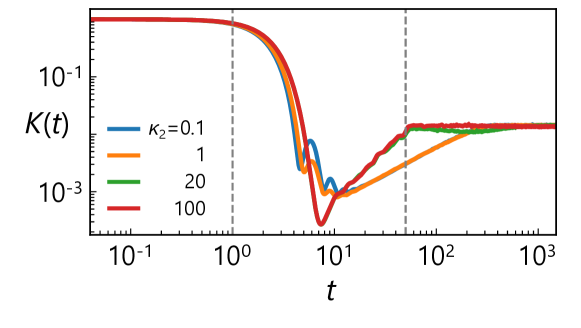
When interpolating between the two models, the overall energy scale varies with the coupling strength. To compare QRC performance on an equal footing, we normalize the Hamiltonian by its spectral norm, . This normalization leaves the level spacing ratio invariant, as well the chaotic nature of the system. However, it introduces a uniform prefactor in the temporal domain, affecting the SFF [Eq. (S3)] and the dependency of QRC performance. Figure S4 displays the SFF for the interpolated model after the rescaling. In the quantum chaotic regime (, ), the typical ramp-plateau profiles emerge, while in the integrable regime (, ), the SFF dips and plateaus at much earlier times. Apart from the overall time-scale shift introduced by the Hamiltonian rescaling, these behaviors mirror those of the SYK4 and SYK2 models in Fig. 2(b) of the main text.
In our QRC performance benchmarks (Fig. 4 of the main text), we selected the input time intervals and ; the corresponding times are marked by the dashed lines in Fig. S4. For the quantum chaotic regime, the longer falls within the RMT ramping window, while the shorter one precedes the dip. Similarly for the integrable models, these two times effectively sandwich the dip. These observations validate both the Hamiltonian normalization procedure and our choice of for probing distinct temporal regimes relevant to QRC. It is worth noting that precisely characterizing chaos in the interpolated model via the SFF typically requires a more sophisticated procedure called unfolding [82]. Unfolding recasts the energy spectrum such that it will exhibit a constant level spacing; it is not an operation directly applied to the Hamiltonian itself. We do not employ this procedure because our primary motivation is to characterize QRC performance by focusing on the properties of the original, physically implemented Hamiltonian.
II Dynamics of quantum reservoir system
The QRC protocol consists of signal encoding, reservoir dynamics, read-out, and post-processing (see Fig. 1 of the main text). We briefly overview this protocol here to provide deeper insight into its dynamics. First, for a sequential input , the -th input is encoded into the -site quantum reservoir system by replacing the quantum state at site . The system then evolves unitarily under the Hamiltonian for a duration until the next input. During this evolution, the single-site particle number is measured at subintervals. The resulting read-out signals, along with an additional constant term, form the -dimensional state vector . The final output is obtained through a linear transformation of this vector with the trainable weight .
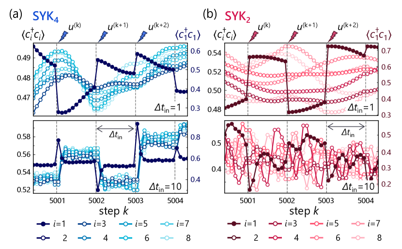
Figures S5(a) and S5(b) illustrate the dynamics of read-out signals for the SYK4 and SYK2 models, respectively, for input intervals of and . The dashed lines indicate when new inputs are provided. Markers show at times (), with the filled marker specifically denoting site , i.e., the input site. The dynamics at the input site change abruptly after an input, showing a larger variation range than other sites; hence, its vertical axis is displayed separately.
With a short input interval (), each new input arrives before the previous one has fully influenced the system. Thus, the resulting dynamics is relatively simple, as shown in the upper panels of both Figs. S5(a) and S5(b). In contrast, system-dependent characteristics emerge when the input interval is longer (). In the SYK4 model [lower panel of Fig. S5(a)], all readout signals tend toward quasi-stationary values, whereas in the SYK2 model [lower panel of Fig. S5(b)], the signals exhibit continuous oscillations. Notably, although both dynamics appear sufficiently rich, their QRC performance differs significantly, as demonstrated in Figs. 3(c) and 3(d) of the main text. Because the output is computed from these readout signals, this performance gap must originate from the difference in dynamics; however, the underlying reason is not immediately obvious from the raw signals in Fig. S5.
These -dependent behaviors raise interest in the relationship between QRC performance and scrambling time—the timescale over which information delocalizes [73]. Since scrambling relates to the propagation of encoded input information, its connection to memory performance is naturally anticipated [35]. Accordingly, the observed dependence of STM performance [upper panels of Figs. 3(c) and 3(d) of the main text] could plausibly reflect the underlying scrambling timescale. Indeed, their similar scaling complicates the precise distinction between the individual contributions of scrambling time and Thouless time. However, the pronounced enhancement in nonlinear processing performance [lower panel of Fig. 3(c) of the main text] cannot be explained by scrambling alone, which is primarily associated with memory. Moreover, the convergence of QRC performance toward that of the Haar QRC model when exceeds the Thouless time underscores a fundamental connection to RMT. These observations collectively suggest that the Thouless time plays the more decisive role in determining overall QRC performance. Nevertheless, the detailed relationship between scrambling time, Thouless time, and the temporal edge of many-body quantum chaos warrants further investigation.
III Convergence property
We here examine echo state property (ESP), a fundamental characteristic of RC systems. ESP dictates that the reservoir state should asymptotically converge when driven by the same input sequence, irrespective of its initial conditions. In other words, after sufficiently many input injections, any dependence on the initial state should vanish. In QRC paradigms, ESP is typically assessed by measuring the distance between two quantum states, and . These states evolve from different initial states, and , but under an identical input sequence. ESP is considered satisfied when this distance approaches 0. Under purely unitary dynamics, the distance between these states, evaluated using the Frobenius norm, remains constant over time: . Thus, the specific time within a unitary evolution step is irrelevant. However, the distance does change upon the nonunitary input injection process, which involves the partial trace over site and the reinitialization with the input state . Consequently, to evaluate ESP, we monitor the state distance as a function of the input step . As the system traces out the previous state and injects a new, identical input state for both trajectories, the distance between and is expected to decrease with . The precise convergence behavior depends on the state before the input and the time evolution process . For instance, if the input interval is close to zero (), the newly added input state is traced out almost immediately, and the distance remains largely unchanged. Conversely, a larger yields more intricate dynamics, where the partial trace operation can lead to a more significant reduction in distance, the details of which depend on the Hamiltonian.
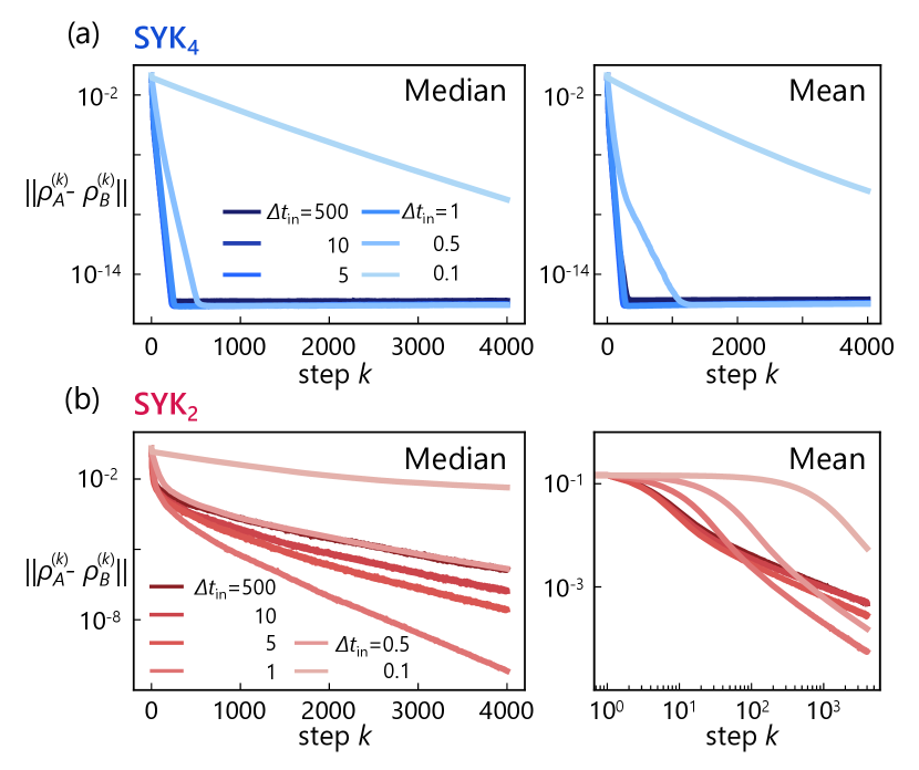
Figures S6(a) and S6(b) display the distance as a function of the input step for various input intervals in the SYK4 and SYK2 models, respectively. The initial states are randomly sampled from the half-filling sector. To accommodate values spanning several orders of magnitude, both the mean and median distances over pairs of initial states are presented. For all models investigated, our results strongly indicate that the update rule [Eq. (2) of the main text] is contractive for random initial conditions and inputs: . This observation suggests that ESP is satisfied for these systems—at least asymptotically as .
Notably, the convergence speeds of the SYK4 and SYK2 models differ significantly. In the SYK4 model, the distance metric consistently decays exponentially toward , but the decay rate is sensitive to the input interval . For smaller intervals (, ), both the mean and median distances converge relatively slowly due to less effective erasure of past states upon the partial trace. Conversely, larger values result in much faster convergence, with the distance behaving similarly across these larger input intervals. In stark contrast, the SYK2 model exhibits considerably slower distance decay. While its median distance also decreases exponentially, the mean distance decays only polynomially and remains relatively high. This behavior reflects the integrable nature of the SYK2 model, wherein numerous internal conserved quantities can impede convergence. These conserved quantities also generate large statistical fluctuations, which explains the disparity between the mean and median distances [Fig. S6(b)] and the large standard deviation in the performance metric (the SYK2-dominated regime in Fig. 4 of the main text).
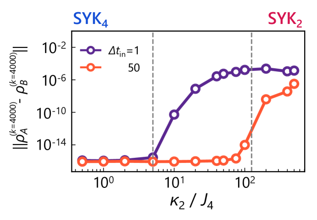
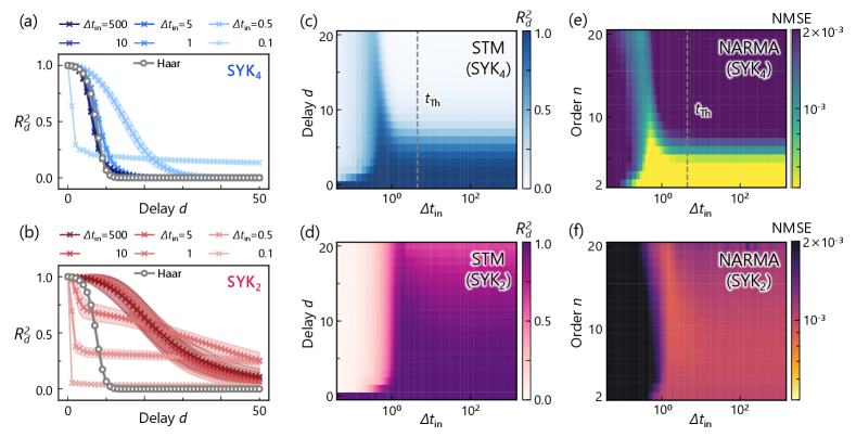
Figure S7 displays the median distance for the interpolated model as a function of the coupling strength . The distance is evaluated at the final step considered () and is presented for two input intervals: and . Larger final distances indicate slower convergence, whereas smaller ones suggest rapid decay. Consistent with Figs. S6(a) and S6(b), the distance approaches for small and remains relatively large in the strong regime for both input intervals. However, the behavior differs between the two input intervals at intermediate values. For , the distance deviates from at relatively small , near the onset of WD statistics. In contrast, with , it stays close to until approaches the boundary of the Poisson regime. This comparison indicates that convergence becomes harder to achieve as the system nears the integrable regime, which requires a large to generate the necessary complex dynamics.
We note that the authors in Ref. [20] discuss QRC performance in spin-based quantum reservoirs, attributing poor performance in localized phases to slow convergence. Our QRC likewise exhibits slow convergence in the SYK2-dominant regime (Fig. S7). However, a crucial difference exists: the QRC in Ref. [20] performs poorly in both linear memory and nonlinear processing within the localized phase, whereas our QRC maintains robust memory performance in the integrable regime [Fig. 3(d) of the main text]. Furthermore, for , the parametric edge of many-body quantum chaos [Fig. 4(a) of the main text] appears at values almost an order of magnitude smaller than those at which the distance metric first deviates from in Fig. S7. This disparity seems to suggest that convergence and the parametric edge are not directly related in the model under investigation.
IV Reservoir performance
The main text presents QRC performance on the short-term memory (STM) task and the nonlinear auto-regressive moving average (NARMA) task. Specifically, it benchmarks the SYK4 [Fig. 3(c)] and SYK2 [Fig. 3(d)] models in the temporal domain, as well as the interpolated model in the parametric domain at input intervals of [Fig. 4(a)] and [Fig. 4(b)]. The aim here is to provide additional data to further elucidate QRC performance and the edge of many-body quantum chaos.
IV.1 Reservoir performance for the SYK4 and SYK2 models
This section examines the detailed QRC performance of the SYK4 and SYK2 models in the temporal domain. We first analyze performance on the STM task, which quantifies linear memory capability. Figures S8(a) and S8(b) present the memory performance as a function of delay for each model, while the input interval is varied. The performance of the Haar QRC model is included for baseline comparison. For the SYK4 model, the performance approaches the Haar QRC reference value at large , reflecting a universal RMT description when exceeds the Thouless time . Optimal performance in this plot occurs at , before the Thouless time, where a long tail of nonzero extends to . Conversely, a very short input interval () yields poor performance, with remaining around even at large . This degradation arises because the partial trace provides less effective memory erasure for such short input intervals, leading to the slow convergence observed in Fig. S7(a).
The tendency of short input intervals to introduce atypical decay in is more pronounced in the SYK2 model [Fig. S8(b)]. For instance, at , the memory performance drops abruptly instead of decaying gradually as in the Haar QRC reference. This behavior suggests a compromised fading-memory property; due to the slow convergence, the system fails to sufficiently prioritize recent information. Nevertheless, for longer input intervals (, , and ), QRC with the SYK2 model demonstrates significantly better memory retention than the Haar QRC baseline, with a long tail spanning beyond . Importantly, this enhancement appears even though the convergence speed [quantified by in Fig. S6(b)] is comparable to that observed at shorter . This discrepancy implies that, while the distance-based convergence metric is valuable for characterizing QRC systems, its direct connection to performance can be system-dependent. Specifically, in the SYK2 model, ESP is satisfied only asymptotically, and it remains nontrivial to determine how this asymptotic nature precisely affects performance. Further investigation, potentially employing alternative convergence metrics, is left for future work.
Figures S8(c) and S8(d) extend Figs. S8(a) and S8(b) respectively, by presenting heatmaps of for as the input interval is varied. In the SYK4 model [Fig. S8(c)], a key observation is an oblique line of high performance that appears where is shorter than the Thouless time. This sharp feature represents the performance enhancement at the temporal edge of many-body quantum chaos, consistent with the observation in Fig. 3(c) of the main text. Since the Thouless time marks the point at which the QRC performance converges to that of the Haar QRC model, any enhancement should occur for below this time. The exact location of the peak is task-dependent; for the task investigated here, it weakly depends on , leading to the observed oblique line. Remarkably, a similar enhancement is absent in the SYK2 model [Fig. S8(d)]; instead, it shows a binary separation between a regime of sufficient memory retention at large and poor retention at small , lacking any distinct performance peak.
Figures S8(e) and S8(f) show heatmaps of the NMSE for the NARMA tasks using the SYK4 and SYK2 models, respectively. The vertical axis shows the NARMA order , and the horizontal axis indicates the input interval . Consistent with the STM task results, a distinct performance peak is evident in the SYK4 model, whereas the SYK2 model shows only gradual performance changes. As discussed in the main text, the absence of peak-like structures in the SYK2 model supports the interpretation that the performance enhancement observed in the SYK4 model indeed originates from many-body quantum chaos. This enhancement persists for larger STM delays and NARMA orders ; although the peak broadens as task complexity increases, the overall observation confirms the robustness of the performance boost induced by the temporal edge.
IV.2 Reservoir performance for the interpolated model
Next, we analyze QRC performance of the model interpolating between the SYK4 and SYK2 systems in Fig. S9, extending the results presented in Fig. 4 of the main text.
Figures S9(a) and S9(b) illustrate the memory performance as a function of delay for various coupling strengths at . For comparative purposes, the performance of the Haar QRC model is also plotted. In the long time-scale regime (), the QRC performance within the quantum chaotic regime () aligns with the Haar QRC reference value, which is a direct consequence of universal RMT behavior [Fig. S9(a)]. As the coupling strength increases, the STM performance improves monotonically, eventually exhibiting an extended tail in in the integrable regime (). This trend is further elucidated in the corresponding heatmap in Fig. S9(c), which plots against the coupling strength ratio (horizontal axis) and delay (vertical axis). The onsets of the chaotic and integrable regimes are indicated by gray dashed lines. Within the quantum chaotic regime, the performance is nearly uniform across , showing a similar dependence on delay . Upon entering the intermediate regime, gradually improves towards the integrable regime, where memory retention is strongest. The boundary separating high (red) and low (blue) values forms an oblique line, indicating that stronger coupling is necessary to preserve memory for longer delays .
By contrast, in the short time-scale regime (), displays a markedly different pattern: a sharp initial drop followed by a slow decay, the decay rate of which diminishes further as the system approaches the integrable limit at large [Fig. S9(b)]. The heatmap in Fig. S9(d) corroborates this observation: a region of high (red) is concentrated at small delays (bottom), illustrating the initial high performance before an abrupt drop. The subsequent slow decay corresponds to the upper regions of nearly uniform, low (blue). These behaviors are attributed to the less effective memory erasure via the partial trace operation when the input interval is short, as discussed previously.
We additionally present performance heatmaps for the NARMA task in Fig. S9(e) for and Fig. S9(f) for . The horizontal axis represents the coupling strength , and the vertical axis shows the NARMA order . For small NARMA orders with a long input interval [Fig. S9(e)], the performance is distinctly enhanced around the chaotic boundary, corresponding to the parametric edge of many-body quantum chaos. This edge-induced performance enhancement is absent for the short input interval in Fig. S9(f) because, as discussed in the main text, the QRC requires a sufficiently long input interval to manifest its quantum chaotic characteristics.
A comparison between the STM task [Fig. S9(c)] and the NARMA task [Fig. S9(e)] illuminates distinct aspects of performance enhancement. Specifically, for small values of and , the NARMA performance displays a pronounced peak around the chaotic boundary, whereas the STM performance shows no comparable improvement. Given that the NARMA task requires both memory and nonlinear processing, we conclude that enhancements in nonlinear transformation, rather than memory, primarily drive the observed performance boost at this parametric edge. As the NARMA order increases, however, the task requires more memory, and memory capacity becomes the dominant performance factor. Consequently, the NARMA performance displays an oblique contour in the high- region, similar to the STM performance, and the edge-induced peak is gradually obscured.