EdgeVO: An Efficient and Accurate Edge-based Visual Odometry
Abstract
Visual odometry is important for plenty of applications such as autonomous vehicles, and robot navigation. It is challenging to conduct visual odometry in textureless scenes or environments with sudden illumination changes where popular feature-based methods or direct methods cannot work well. To address this challenge, some edge-based methods have been proposed, but they usually struggle between the efficiency and accuracy. In this work, we propose a novel visual odometry approach called EdgeVO, which is accurate, efficient, and robust. By efficiently selecting a small set of edges with certain strategies, we significantly improve the computational efficiency without sacrificing the accuracy. Compared to existing edge-based method, our method can significantly reduce the computational complexity while maintaining similar accuracy or even achieving better accuracy. This is attributed to that our method removes useless or noisy edges. Experimental results on the TUM datasets indicate that EdgeVO significantly outperforms other methods in terms of efficiency, accuracy and robustness.
I Introduction
Visual Odometry (VO), which estimates the camera motion from a stream of images, plays an important role in many applications, such as augmented reality (AR), autonomous vehicles, and robot navigation [1, 2, 3]. Popular VO methods include salient feature-based approaches [4, 5] and direct methods [6, 7, 8]. Feature-based methods obtain the motion estimation by extracting and matching feature points, while direct methods track the camera based on photometric or geometric error [9, 10, 11]. Feature-based methods are advantageous of being insensitive to brightness change, but are heavily dependent on the textures and computationally expensive. By contrast, direct methods do not require salient texture features and are more computation-friendly, but they are more sensitive to brightness change and vulnerable to local optimum.
Although many efforts have been made to improve the performance of visual odometry, it is challenging to estimate the camera motion in some corner cases [13, 14]. For example, textureless scenes cannot provide sufficient feature points for salient feature-based approaches, and sudden illumination changes can cause the assumption invalidation of photometric consistency for direct methods. These factors reduce the effectiveness of the VO algorithm or even cause tracking failure [15, 16]. To overcome these drawbacks, several solutions have been proposed. Some combine various features, such as lines [17, 18] and planes [19, 20, 21], to track the pose of the camera. Another solution is to improve direct methods by using affine lighting correction [7], photometric calibration [8], and descriptor fields [22] to handle the illumination changes. Multi-metric fusion approaches [23, 24] combine geometric and photometric to improve the accuracy and robustness of camera tracking to a certain extent.
As another attempt, the recently emerging edge-based methods [12, 16, 25, 26] have shown robust performance in these corner cases. They employ image edges that are observed more naturally and stably in textureless environments, and apply 3D-2D edge registration to estimate the pose of a camera. Compared to feature-based and direct methods, edge-based methods can work in both textureless scenarios and environments with brightness changes. However, there are still some challenges remained in edge-based VO approaches. It is known that edge alignment is less accurate due to the absence of dedicated descriptors for edges, thus producing much higher outlier rates [26]. To improve the accuracy of pose estimation, most edge-based systems exploit a large amount of measurements to solve a nonlinear least-squares problem [27, 28, 29]. In each iteration of pose optimization, the nearest neighbor searching is performed multiple times, which drastically increase the computational complexity of such method.
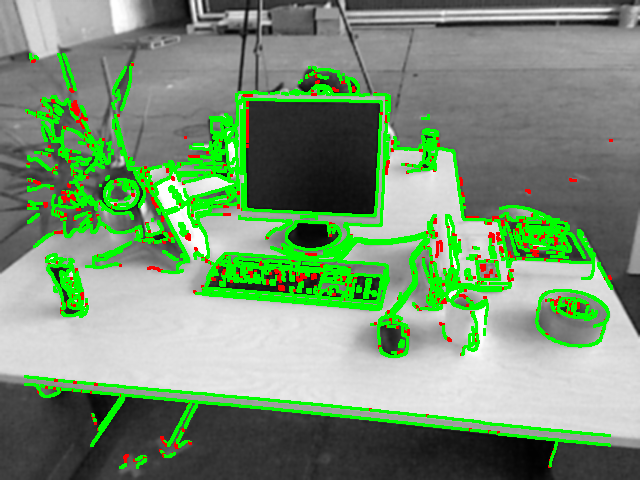
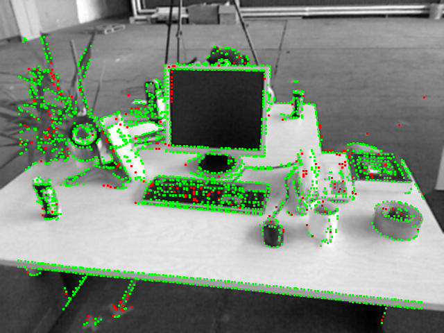
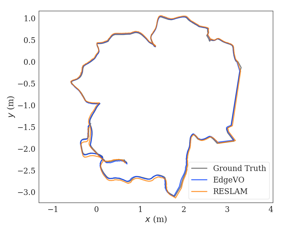
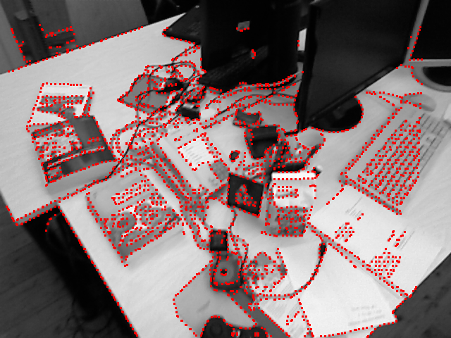
In this paper, we propose a novel method, which is called EdgeVO, for the pose estimation of the camera. Unlike existing edge-based approaches, which use all extracted edges, we use only a small subset of the extracted edges that are selected according to their contribution to motion estimation. Then, we track only the selected edges to estimate camera motion. More specially, we formulate edge selection as a submatrix selection problem, and then use an efficient greedy algorithm to approximate optimal results with considering spatial correlation and observational uncertainty. Our approach is proven to achieve computational complexity with 1/2 approximation guarantee. Figure 1 gives an illustration of the proposed EdgeVO with RESLAM [12].
Compared to existing edge-based methods, our method can significantly reduce the computational complexity while maintaining similar accuracy or even achieving better accuracy since our method removes useless or noisy edges. Figure 1 compares the number of extracted features, estimated trajectory, and accuracy vs time of EdgeVO and popular RESLAM. We have also conducted experiments on the TUM datasets, experimental results on the TUM datasets indicate that EdgeVO significantly outperforms other methods in terms of efficiency, accuracy and robustness.
II Problem Formulation
For each incoming frame , we use the iterative closest points (ICP)-based algorithm to estimate the camera motion relative to its reference frame by aligning their respective edges pixel. The edge alignment is performed by re-projecting valid edge pixel set from to and minimizing the distance to the closest edge pixels in . To speed up edge alignment, we first compute the distance field of using Distance Transform [30]. For an edge pixel with inverse depth in reference frame, the re-projected distance residual under the transformation is defined as:
| (1) |
where is a warping function for re-projecting the edge from to , and is the perspective projection function.
We arrange all residuals of valid edges in the reference frame into one column vector. The residual vector can be formulated as . The optimal relative camera motion is estimated by minimizing the sum of squared residuals:
| (2) |
where is a weighting matrix. We use a Huber weighting scheme to reduce the influence of large residuals.
Iterative methods such as Gauss-Newton or Levenberg-Marquardt are often used to solve the nonlinear least squares problem. In each iteration, they perform a first-order linearization of about the current value of by computing the motion Jacobian , and then solve the linear least-squares problem to update the motion, namely
| (3) |
At the final iteration, the least-squares covariance of the motion estimation is calculated as , which reveals the uncertainty of motion estimation. Generally, it depends on the spectral properties of , if we use more valid edges to track, the singular values of would increase in magnitude, and the accuracy of motion estimation is more likely to be improved [31].
However, the number of edges detected in each frame are very large (e.g., tens of thousands), and using all of them would greatly reduce computational efficiency. In this paper, we try to use only a small subset of the edges to speed up motion estimation while preserving the accuracy and robustness. As suggested in [31], we aim to find a submatrix (i.e., a subset of row blocks) in that preserves the overall spectral properties of as much as possible.
Now, we formulate the edge selection problem. Let be the indices of row blocks in full matrix and . denotes the index subsets of selected row blocks, is the corresponding concatenated submatrix, and is the number of selected row blocks. Then, the submatrix selection problem is formulated as:
| (4) |
where logdet() is a submodular function to compute the log determinant of a matrix, which quantifies the spectral properties of the matrix.
It is known that the submodular optimization problem is NP-hard, the stochastic greedy method [31, 32, 33] is commonly used to provide a near-optimal solution with an approximation guarantee. It starts with an empty set, and in each round , it randomly samples a subset . Then, it picks up an element with maximizing the marginal gain:
| (5) |
III Proposed Method: EdgeVO
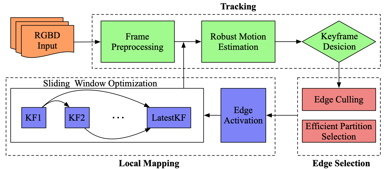
The architecture of EdgeVO is demonstrated in Figure 2. It consists of two parallel threads: tracking, and local mapping. The tracking thread estimates the relative camera motion between the current frame and the latest keyframe and then decides if a new keyframe should be created. If a new keyframe is created, we propagate it to the local mapping thread and refine the relevant state variables using the sliding window optimization. The edges are selected for each keyframe, which are used for both relative motion estimation and local optimization. Next, we elaborate on each key component.
III-A Tracking
In order to estimate the camera relative motion, we firstly preprocess each frame to get the edges image and distance field pyramid. Then, a coarse-to-fine robust optimization is performed for edge alignment based on the distance field pyramid. Finally, we decide whether a keyframe is created according to the alignment status. In the following, we will provide more details of these steps.
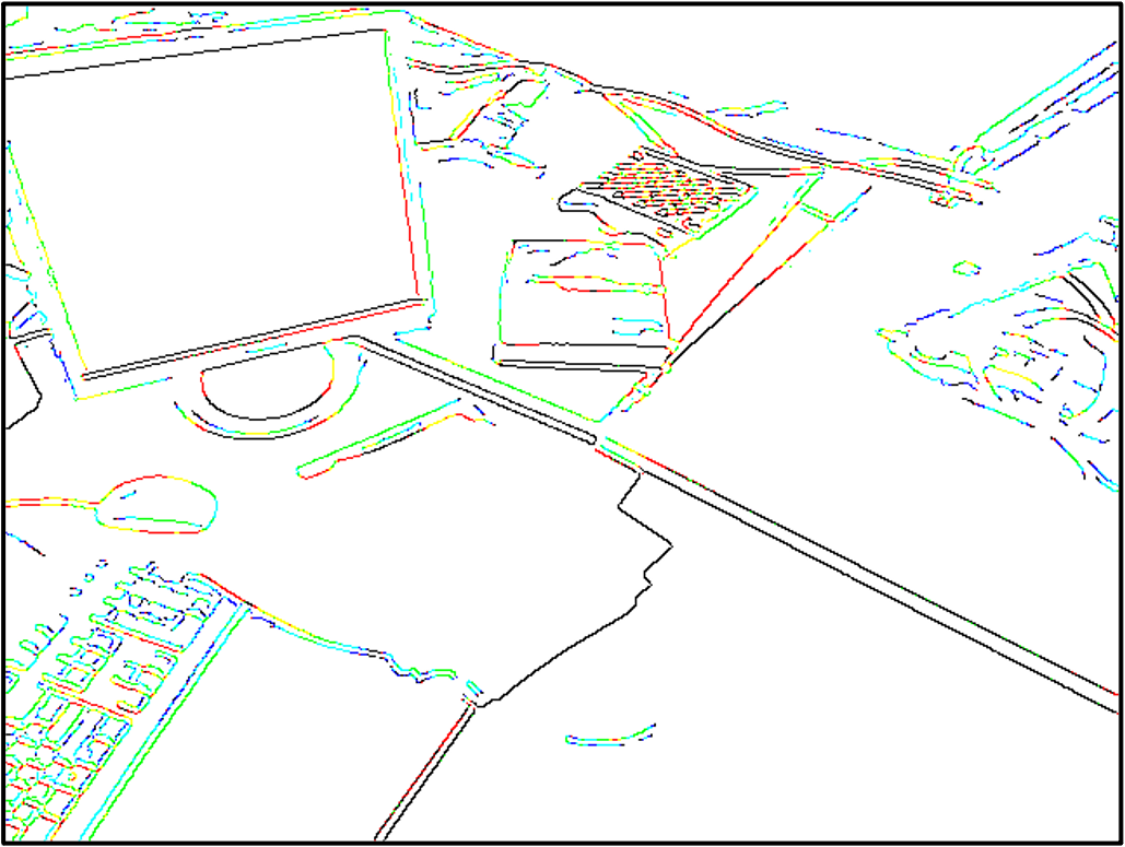
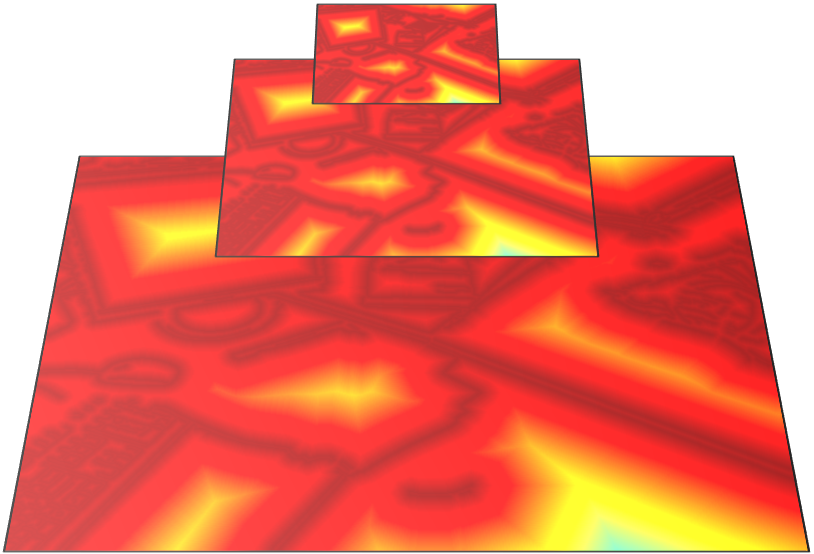
Frame Preprocessing As shown in Figure 3, when the current frame comes, we first detect edge pixels using the Canny algorithm [34]. It works well in low-texture and illumination changes scenes because it locally finds the strongest edges by non-maximum suppression of high gradient regions. Then, we compute the distance field of the edge image, and create a three-level distance field pyramid for achieving robust optimization of edge alignment. Instead of alternately performing edge detection and distance transform, we directly generate low-resolution distance field by downscaling from the highest resolution level by linear interpolation [12].

Robust Motion Estimation The relative camera motion between the current frame and the latest keyframe is estimated within the ICP framework. Specifically, we use only the selected edges in , and adopt a coarse-to-fine optimization scheme with the distance field pyramid to handle the large displacement. The edge re-projection and alignment are layer-by-layer performed from the lowest resolution level to the highest level. After final iteration, the optimal camera relative motion is obtained.
In order to improve the robustness and accuracy of camera tracking, we try to identify and remove potential outliers in each iterative optimization. The specific process is as follows. First, the residual terms that exceed a certain threshold are removed from the objective function described in equation (2). We set the threshold separately for each level in the distance field pyramid. Second, if a pair of putative edge correspondences is reasonable, their gradient directions should be as consistent as possible under the assumption that there is no large rotation between and . Note that the closest edge coordinate is additionally retained in extracting the distance field. We reproject an edge pixel from to and query its closest edge . Then, the matched pair is regarded as outliers if the inner product of their gradient directions is under a certain margin:
| (6) |
where is the normalized image gradient on the edge pixel. A larger threshold means stricter requirements for consistency, which is empirically set to 0.6 in this work.
Keyframe Decision In general, well-distributed keyframes are very important to ensure the performance of the whole system. Similar to [8], we use the following criteria to decide whether the current frame will be selected as a keyframe: (i) We use the mean squared error of optical flow from the last frame to the latest frame to measure the changes in the field of view and the mean flow without rotation to measure the occlusions. The current frame is selected as keyframe, if , where , provide a relative weighting of two indicators. (ii) If the number of edge correspondences between and is below thirty percent of the average edge correspondences, we treat the current frame as a new keyframe. (iii) If none of the previous conditions occur, we insert new keyframe in a fixed interval (1 second).
III-B Edge Selection
To increase the efficiency of EdgeVO, a small subset of edges is selected from each new created keyframe, and used for tracking subsequent frames and local mapping. We first cull the useless and spurious edges, and then solve the submatrix selection problem to guide edge selection. Specially, we propose an efficient partition selection approach to make the selection more efficiently and robustly.
Edge Culling The edges detected by the Canny algorithm are usually redundant. We thus cull a part of the edges to reduce the size of the ground set before edge selection. First, the edges without depth information are culled since they cannot be directly used for re-projection. Then, we filter out the edges whose gradient magnitude is lower than the high threshold in the Canny algorithm. Only the edges with higher gradient will be retained since they have high signal-to-noise ratio, which is more likely to be beneficial for more accurate motion estimation.
Efficient Partition Selection To avoid the clustering of selected edges, we optimize the submatrix selection problem over a partition matroid. Specifically, the indice set of row blocks in full matrix is divided into disjoint partitions, where , and the edges with the constraint are selected. We denote as a set of all feasible solution , as the partition matroid. The edge selection problem is reformulated as:
| (7) |
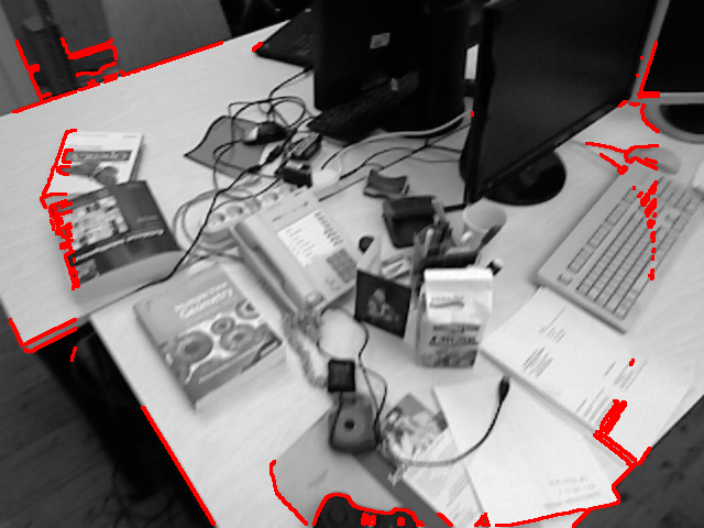
where is the Hessian matrix of the edges. We impose an imaginary grid on the image and count the edges in each grid to build partitions. This forces the selected edges to spread evenly over the whole image as seen in Figure 4.
In order to reduce the computational complexity of submatrix selection, we design a special approximation algorithm, namely Stochastic Partition Greedy. At the -th iteration, we randomly pick up a partition from . Then, an edge is selected from the partition when the following condition holds:
| (8) |
where is the subset selected at previous iteration. The introduction of diagonal matrix is to improve its numerical stability. In this way, each edge is computed only once, and the complexity is thus reduced to .
Proposition 1 We use to denote the optimal solution for the problem (7), and use to denote the approximation solution provided by Stochastic Partition Greedy. The approximation guarantee is thus .
In order to avoid invalid selection, we first assume that if the edge is re-observed in the current frame, it is valid to constrain the motion estimation. We model the case by introducing a Bernoulli distribution , where is a binary variable. means that the -th edge is re-observed in the current frame, while means that such edge is absent in the current frame. Then we re-write the submodular function as,
| (9) |
It is clear that if the edge is re-observed, then and it is able to provide valid marginal gain. Otherwise, this marginal gain simply disappears and we try to find other valid edges to maximize the function. Since is a random variable, the value of the function logdet is a stochastic quantity. Hence, we should maximize the expectation of this function. Let denote the probability of the edge being re-observed, and we have that,
| (10) |
We can judge whether an edge is re-observed or not from two aspects. First, as the camera moves, some edges extend beyond the camera’s field of view, and it would not be re-observed for the subsequent frames. In the practice, we perform the visibility check and filter out these invisible edges based on the prior camera motion. Then, the more distinctive the appearance of the edge, the more likely it is to be re-observed. Thus, we model the probability of the edge being re-observed as,
| (11) |
where is the high threshold in the Canny algorithm, and is the gradient magnitude of the edge .
In this way, the gradient magnitude of an edge is larger than the high threshold. It is thus more likely to be detected by the Canny algorithm in the next frames, which is a desired behavior. Finally, we provide the pseudo-code of the complete edge selection approach in Algorithm 1.
III-C Local Mapping
To improve the consistency of the camera trajectory, we maintain a small local window of keyframes in the local mapping component, where is set to a value between 5 and 7. For each new keyframe, the edges that satisfy certain criterions in the window are activated to create new geometric constraints, and then we perform a sliding window optimization to jointly refine the inverse depths of all active edges, global camera poses and the intrinsic within the window. The specific steps of local mappings are as follows.
Edge Activation When a new keyframe is added, we use it to activate the edges of the previous keyframes in the window. In order to obtain the evenly distributed edges and reliable geometric constraints, we divide the image in cells into fixed size (e.g., pixels). We then reproject all edges into these grids, while the active edges are selected from each cell. The following criterions need to be satisfied at the same time to activate an edge:
-
1.
The candidate edge’s geometric residual cannot exceed a certain threshold, which is set to the median of all residuals;
-
2.
The reprojected gradient direction of the candidate edge should be as consistent as possible with the image gradient direction of its closest edge in the new frame. We set the angle between the two directions to be in the range ;
-
3.
The edges that are tracked for longer period of time are considered to be more reliable. Therefore, we count the number of times each edge was successfully tracked and select the older one as the active edge;
Silding Window Optimization For the keyframe , in the window, the geometric residuals are computed by reprojecting the active edges in into ,
| (12) |
where is the projected position of in the keyframe , and , are the estimated camera poses relative to the world frame. All state variables in the window are denoted by . The optimal state vector is estimated through minimizing the overall residuals over the window:
| (13) |
We fix the bound size of the local window. One of previous keyframes need to be marginalized before adding a new one. Following [8], we keep the latest two keyframes in the window, and marginalize a keyframe if it is further away from the newest one or it has less edges visible in others. Before marginalizing one keyframe, we first adapt the marginalization strategy with the Schur complement to marginalize its active edges and the edges that are not observed in the last two keyframes. This is to retain the sparsity of our method.
IV Expriments and Results
IV-A Experimental Setup
In this section, we evaluate the performance of our method on the standard RGBD benchmark dataset–TUM RGBD [35], which is widely used for evaluating various RGBD VO and SLAM algorithms. The dataset provides synchronized RGB images and depth images recorded with a Microsoft Kinect v. sensor at Hz. The ground truth trajectories are obtained by a motion capture system. All experiments are implemented on a desktop computer with an Intel CPU of i CPU and a RAM of GB.
| Sequence | ElasticFusion | ORB-SLAM2 | Canny-VO | RESLAM | Ours |
|---|---|---|---|---|---|
| fr1_desk | 0.020 | 0.016 | 0.044 | 0.036 | 0.018 |
| fr1_desk2 | 0.048 | 0.030 | 0.187 | 0.063 | 0.046 |
| fr1_floor | 0.021 | 0.040 | 0.033 | ||
| fr1_rpy | 0.025 | 0.031 | 0.047 | 0.048 | 0.037 |
| fr1_xyz | 0.011 | 0.020 | 0.043 | 0.024 | 0.009 |
| fr2_desk | 0.071 | 0.027 | 0.037 | 0.034 | 0.023 |
| fr2_rpy | 0.015 | 0.003 | 0.007 | 0.006 | 0.006 |
| fr2_xyz | 0.011 | 0.005 | 0.008 | 0.005 | 0.003 |
| fr3_office | 0.017 | 0.021 | 0.085 | 0.078 | 0.033 |
| fr3_nostr_tex_near | 0.016 | 0.030 | 0.090 | 0.199 | 0.026 |
| fr3_str_notex_far | 0.030 | 0.031 | 0.084 | 0.024 | |
| fr3_str_tex_far | 0.013 | 0.012 | 0.013 | 0.015 | 0.011 |
| fr3_str_tex_near | 0.015 | 0.014 | 0.025 | 0.013 | 0.012 |
| fr3_cabinet | 0.057 | 0.058 | 0.024 |
IV-B Experimental Results
We compare the proposed EdgeVO with several baseline methods in terms of accuracy, robustness and efficiency. These baseline methods range from direct methods, feature-based methods, to edge-based methods. The specific baseline methods selected are as follows:
-
1.
ElasticFusion [23] is a map-centric SLAM approach, which combines geometric and photometric error for frame-to-model pose estimation.
-
2.
ORB-SLAM2 [5] is a feature-based SLAM approach, which estimates camera motion based on feature matches.
-
3.
Canny-VO [26] is an edge-based visual odometry method. It adapts the approximate nearest neighbor fields or oriented nearest neighbor fields to estimate camera relative motion.
-
4.
RESLAM [12] is the first open-source edge-based SLAM system, where the camera motion is estimated based on Euclidean distance fields.
Note that the odometry and mapping are separated in the methods of ORB-SLAM2 and RESLAM. We deactivate the loop modules for fair comparison, and the results of Canny-VO [26] and ElasticFusion [23] are directly taken from the original papers. We run ORB-SLAM2 and RESLAM on computing platform and report their performance.
Estimation Error We first compare the achieved error of EdgeVO with the selected baseline methods. The Root Mean Squared Error (RMSE) of the translational component of the Absolute Trajectory Error (ATE) is taken as the performance metric. The results are shown in Table I, from which we can see that the proposed EdgeVO performs the best. It witnesses a lower error than all the baseline methods in most cases. We can also find that EdgeVO performs much better than other edge-based methods, namely Canny-VO and RESLAM. There are two potential reasons why our method outperforms the two edge-based methods. The first reason is that we remove the potential outliers based on appearance similarity, and activate the edges that are more reliable to optimize the camera motion, which are not considered in Canny-VO and RESLAM. The other reason is that we use only a small number of edges that are selected with a certain strategy since too many edges and uneven distribution may lead to unstable optimization values, and the edge selection could further improve the accuracy. EdgeVO also generally outperforms ORB-SLAM2 and ElasticFusion especially in textureless scenarios, while it performs slightly worse than ORB-SLAM2 and ElasticFusion in feature-rich environments.
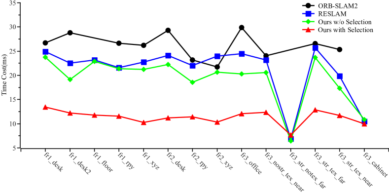
Efficiency Then, we compare the computational efficiency of EdgeVO with the baseline methods. We calculate the average running time per frame of ORB-SLAM2, RESLAM and our method on each sequence, the results are shown in Figure 5. It is clear that the proposed EdgeVO has the lowest time cost and could achieve about Hz reporting the result on the majority of sequences, due mainly to the fact that we use only a small subset of edges in the tracking and local mapping. If our method use all edges the same as RESLAM does, then the time costs of the two method are close. Compared to the edge-based methods including EdgeVO and RESLAM, ORB-SLAM2 requires feature matches based on the similarity of descriptors and additionally frame-to-model pose optimization, so its computational cost is the highest. Compared to ElasticFusion that requires a GPU and achieves a frequency of Hz for motion estimation, our method is about four times faster in terms of the computing speed even using only a i CPU. Since Canny-VO is not open-sourced, we directly use the frequency of reporting estimation result, which is about Hz even using a i CPU which is higher in configuration than the CPU we used. Yet, our method is still more efficient than Canny-VO. In addition, the computational cost of our method is close to that of RESLAM in fr3_str_notex_far and fr3_cabinet. This is because the number of edges is inherently less, and edge selection has to keep most of the edges to sufficiently constrain the motion estimation.
Robustness Here, we qualitatively evaluate the robustness of the baseline methods based on their tracking failures. From the Table I, we can find that edge-based methods work successfully for each sequence, while ORB-SLAM2 and ElasticFusion fail in some cases. In detail, the tracking of ORB-SLAM2 is lost in the sequences with sudden motion fr1_floor and poor texture (fr3_str_notex_far, fr3_cabinet), since there are not sufficient and reliable feature matches for tracking. For ElasticFusion, sudden motion makes the optimization difficult to converge. Besides, illumination changes (fr2_desk) and high reflection (fr3_cabinet) negatively affect the photometric-based optimization. Thus, ElasticFusion fails sometimes in tracking or results in a low accuracy in these scenarios. While these limitations do not exist on edge-based methods, the edges in these sequences are sufficient even under poor texture scenes. The optimization based on distance field paradigm has a larger radius of convergence and is insensitive to illumination changes, so edge-based methods show better robustness than ElasticFusion and ORB-SLAM2 in these scenarios.
IV-C Abalation Study
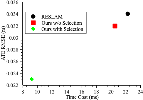
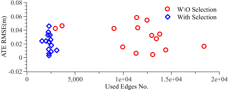
In this section, we evaluate the effectiveness of the proposed edge selection method by reporting the performance of EdgeVO with and without edge selection. As can be seen from Figure 5, EdgeVO with edge selection has lower running time compared to the one without selection. Additionally, we compare the number of used edges and the resulted RMSE of the translational ATE in each sequence. The results are shown in Figure 6, where each point represents the performance on a sequence. It is clear that our system with edge selection utilizes less edges and achieves similar or higher accuracy than that without selection.
V Conclusion
In this paper, we propose an accurate, efficient and robust approach for edge-based visual odometry using RGBD cameras, which is called EdgeVO. It can significantly reduce the number of edges required for motion estimation, and result in great computational efficiency improvement over existing edge-based methods without sacrificing accuracy and robustness. We evaluate the proposed method on the public TUM RGBD benchmark, finding that it performs better than state-of-the-art methods with respect to efficiency, accuracy and robustness. For future work, we will investigate large-scale camera motion estimation as well as loop closure for edge-based methods.
Acknowledgement
This work was supported by the National Natural Science Foundation of China (No. 42174050, 62172066), Venture & Innovation Support Program for Chongqing Overseas Returnees (No. cx2021047, cx2021063), and Startup Program for Chongqing Doctorate Scholars (No. CSTB2022BSXM-JSX005).
References
- [1] C. Cadena, L. Carlone, H. Carrillo, Y. Latif, D. Scaramuzza, J. Neira, I. Reid, and J. J. Leonard, “Past, present, and future of simultaneous localization and mapping: Toward the robust-perception age,” IEEE Transactions on robotics, vol. 32, no. 6, pp. 1309–1332, 2016.
- [2] T. Taketomi, H. Uchiyama, and S. Ikeda, “Visual slam algorithms: A survey from 2010 to 2016,” IPSJ Transactions on Computer Vision and Applications, vol. 9, no. 1, pp. 1–11, 2017.
- [3] G. Younes, D. Asmar, E. Shammas, and J. Zelek, “Keyframe-based monocular slam: design, survey, and future directions,” Robotics and Autonomous Systems, vol. 98, pp. 67–88, 2017.
- [4] G. Klein and D. Murray, “Parallel tracking and mapping for small ar workspaces,” in 2007 6th IEEE and ACM international symposium on mixed and augmented reality. IEEE, 2007, pp. 225–234.
- [5] R. Mur-Artal and J. D. Tardós, “Orb-slam2: An open-source slam system for monocular, stereo, and rgb-d cameras,” IEEE transactions on robotics, vol. 33, no. 5, pp. 1255–1262, 2017.
- [6] C. Kerl, J. Sturm, and D. Cremers, “Robust odometry estimation for rgb-d cameras,” in 2013 IEEE international conference on robotics and automation. IEEE, 2013, pp. 3748–3754.
- [7] J. Engel, J. Stückler, and D. Cremers, “Large-scale direct slam with stereo cameras,” in 2015 IEEE/RSJ international conference on intelligent robots and systems (IROS). IEEE, 2015, pp. 1935–1942.
- [8] J. Engel, V. Koltun, and D. Cremers, “Direct sparse odometry,” IEEE transactions on pattern analysis and machine intelligence, vol. 40, no. 3, pp. 611–625, 2017.
- [9] R. A. Newcombe, S. Izadi, O. Hilliges, D. Molyneaux, D. Kim, A. J. Davison, P. Kohi, J. Shotton, S. Hodges, and A. Fitzgibbon, “Kinectfusion: Real-time dense surface mapping and tracking,” in 2011 10th IEEE international symposium on mixed and augmented reality. Ieee, 2011, pp. 127–136.
- [10] F. Pomerleau, S. Magnenat, F. Colas, M. Liu, and R. Siegwart, “Tracking a depth camera: Parameter exploration for fast icp,” in 2011 IEEE/RSJ International Conference on Intelligent Robots and Systems. IEEE, 2011, pp. 3824–3829.
- [11] P. Henry, M. Krainin, E. Herbst, X. Ren, and D. Fox, “Rgb-d mapping: Using kinect-style depth cameras for dense 3d modeling of indoor environments,” The international journal of Robotics Research, vol. 31, no. 5, pp. 647–663, 2012.
- [12] F. Schenk and F. Fraundorfer, “Reslam: A real-time robust edge-based slam system,” in 2019 International Conference on Robotics and Automation (ICRA). IEEE, 2019, pp. 154–160.
- [13] Z. Chen, W. Sheng, G. Yang, Z. Su, and B. Liang, “Comparison and analysis of feature method and direct method in visual slam technology for social robots,” in 2018 13th World Congress on Intelligent Control and Automation (WCICA). IEEE, 2018, pp. 413–417.
- [14] Z. Zunjie and F. Xu, “Real-time indoor scene reconstruction with rgbd and inertia input,” arXiv preprint arXiv: 1812.03015, 2018.
- [15] C. Kim, P. Kim, S. Lee, and H. J. Kim, “Edge-based robust rgb-d visual odometry using 2-d edge divergence minimization,” in 2018 IEEE/RSJ International Conference on Intelligent Robots and Systems (IROS). IEEE, 2018, pp. 1–9.
- [16] C. Kim, J. Kim, and H. J. Kim, “Edge-based visual odometry with stereo cameras using multiple oriented quadtrees,” in 2020 IEEE/RSJ International Conference on Intelligent Robots and Systems (IROS). IEEE, 2020, pp. 5917–5924.
- [17] H. Zhou, D. Zou, L. Pei, R. Ying, P. Liu, and W. Yu, “Structslam: Visual slam with building structure lines,” IEEE Transactions on Vehicular Technology, vol. 64, no. 4, pp. 1364–1375, 2015.
- [18] A. Pumarola, A. Vakhitov, A. Agudo, A. Sanfeliu, and F. Moreno-Noguer, “Pl-slam: Real-time monocular visual slam with points and lines,” in 2017 IEEE international conference on robotics and automation (ICRA). IEEE, 2017, pp. 4503–4508.
- [19] R. F. Salas-Moreno, B. Glocken, P. H. Kelly, and A. J. Davison, “Dense planar slam,” in 2014 IEEE international symposium on mixed and augmented reality (ISMAR). IEEE, 2014, pp. 157–164.
- [20] M. Kaess, “Simultaneous localization and mapping with infinite planes,” in 2015 IEEE International Conference on Robotics and Automation (ICRA). IEEE, 2015, pp. 4605–4611.
- [21] L. Ma, C. Kerl, J. Stückler, and D. Cremers, “Cpa-slam: Consistent plane-model alignment for direct rgb-d slam,” in 2016 IEEE International Conference on Robotics and Automation (ICRA). IEEE, 2016, pp. 1285–1291.
- [22] J. Quenzel, R. A. Rosu, T. Läbe, C. Stachniss, and S. Behnke, “Beyond photometric consistency: Gradient-based dissimilarity for improving visual odometry and stereo matching,” in 2020 IEEE International Conference on Robotics and Automation (ICRA). IEEE, 2020, pp. 272–278.
- [23] T. Whelan, S. Leutenegger, R. Salas-Moreno, B. Glocker, and A. Davison, “Elasticfusion: Dense slam without a pose graph.” Robotics: Science and Systems, 2015.
- [24] A. Dai, M. Nießner, M. Zollhöfer, S. Izadi, and C. Theobalt, “Bundlefusion: Real-time globally consistent 3d reconstruction using on-the-fly surface reintegration,” ACM Transactions on Graphics (ToG), vol. 36, no. 4, p. 1, 2017.
- [25] M. Kuse and S. Shen, “Robust camera motion estimation using direct edge alignment and sub-gradient method,” in 2016 IEEE international conference on robotics and automation (ICRA). IEEE, 2016, pp. 573–579.
- [26] Y. Zhou, H. Li, and L. Kneip, “Canny-vo: Visual odometry with rgb-d cameras based on geometric 3-d–2-d edge alignment,” IEEE Transactions on Robotics, vol. 35, no. 1, pp. 184–199, 2018.
- [27] J. J. Tarrio and S. Pedre, “Realtime edge-based visual odometry for a monocular camera,” in Proceedings of the IEEE International Conference on Computer Vision, 2015, pp. 702–710.
- [28] J. J. Tarrio, C. Smitt, and S. Pedre, “Se-slam: Semi-dense structured edge-based monocular slam,” arXiv preprint arXiv:1909.03917, 2019.
- [29] F. Schenk and F. Fraundorfer, “Robust edge-based visual odometry using machine-learned edges,” in 2017 IEEE/RSJ International Conference on Intelligent Robots and Systems (IROS). IEEE, 2017, pp. 1297–1304.
- [30] P. F. Felzenszwalb and D. P. Huttenlocher, “Distance transforms of sampled functions,” Theory of computing, vol. 8, no. 1, pp. 415–428, 2012.
- [31] Y. Zhao and P. A. Vela, “Good feature selection for least squares pose optimization in vo/vslam,” in 2018 IEEE/RSJ International Conference on Intelligent Robots and Systems (IROS). IEEE, 2018, pp. 1183–1189.
- [32] B. Mirzasoleiman, A. Badanidiyuru, A. Karbasi, J. Vondrák, and A. Krause, “Lazier than lazy greedy,” in Proceedings of the AAAI Conference on Artificial Intelligence, vol. 29, no. 1, 2015.
- [33] Y. Zhao and P. A. Vela, “Good feature matching: toward accurate, robust vo/vslam with low latency,” IEEE Transactions on Robotics, vol. 36, no. 3, pp. 657–675, 2020.
- [34] J. Canny, “A computational approach to edge detection,” IEEE Transactions on pattern analysis and machine intelligence, no. 6, pp. 679–698, 1986.
- [35] J. Sturm, N. Engelhard, F. Endres, W. Burgard, and D. Cremers, “A benchmark for the evaluation of rgb-d slam systems,” in 2012 IEEE/RSJ international conference on intelligent robots and systems. IEEE, 2012, pp. 573–580.