eDNAPlus: A unifying modelling framework for DNA-based biodiversity monitoring
Abstract
DNA-based biodiversity surveys involve collecting physical samples from survey sites and assaying the contents in the laboratory to detect species via their diagnostic DNA sequences. DNA-based surveys are increasingly being adopted for biodiversity monitoring and decision-making. The most commonly employed method is metabarcoding, which combines PCR with high-throughput DNA sequencing to amplify and then read ‘DNA barcode’ sequences. This process generates count data indicating the number of times each DNA barcode was read. However, DNA-based data are noisy and error-prone, with several sources of variation. In this paper, we present a unifying modelling framework for DNA-based survey data, for the first time simultaneously allowing for all key sources of variation, error and noise in the data-generating process. The model can be used to estimate within-species biomass changes across sites and to link those changes to environmental covariates, while accounting for between-species and between-sites correlation. Inference is performed using MCMC, where we employ Gibbs or Metropolis-Hastings updates with Laplace approximations. We further implement a re-parameterisation scheme, appropriate for crossed-effects models, leading to improved mixing, and an adaptive approach for updating latent variables, which reduces computation time. We discuss study design and present theoretical and simulation results to guide decisions on replication at different survey stages and on the use of quality control methods. Finally, we demonstrate the new framework on a dataset of Malaise-trap samples. Specifically, we quantify the effects of elevation and distance-to-road on each species, infer species correlations, and produce maps identifying areas of high biodiversity and species biomass, which can be used to rank areas by conservation value. We also estimate the level of noise between sites and within sample replicates, and the probabilities of error at the PCR stage, which are found to be close to zero for most species considered, validating the employed laboratory processing.
Keywords: crossed-effects model, environmental DNA, joint species distribution modelling, observation error, occupancy modelling
1 Introduction
Ecology is undergoing a technology revolution that is making it possible to rapidly generate species inventories via automated and high-throughput DNA sequencers and via electronic sensors, such as drones, satellites, camera traps, and acoustic recorders. These techniques can, if coupled with appropriate algorithms and databases, simultaneously identify large numbers of target species, including those that are cryptic, difficult-to-access, tiny, and low-abundance (Tosa et al.,, 2021; van Klink et al.,, 2022; Bush et al.,, 2017; Besson et al.,, 2022; Piper et al.,, 2019; Ley,, 2022). So far, the most efficient method for generating species-resolution inventories is DNA-based surveys, which rely on reading DNA barcodes: short, standardized sections of the genome that can be compared to a reference library to enable taxonomic identifications without the need to examine organism morphologies (Ratnasingham and Hebert,, 2007).
DNA barcoding refers to the identification of single species (Hebert et al.,, 2003), and DNA metabarcoding refers to the detection of large numbers of species from environmental DNA (eDNA), which is the collective name for DNA isolated from environmental samples (Bohmann et al.,, 2014; Pawlowski et al.,, 2020; Taberlet et al.,, 2018). These environmental samples include water (Thomsen and Willerslev,, 2015), soil (Frøslev et al.,, 2019), air (Clare et al.,, 2022; Lynggaard et al.,, 2022), and bulk tissue (i.e. mass-trapped organisms) (Ji et al.,, 2013). For instance, Thomsen and Sigsgaard, (2019) demonstrated that traces of eDNA on flower petals could be analysed to describe the diversity of arthropods that visit wildflowers, including pollinators, parasitoids, predators, and herbivores. Ji et al., (2022) used the trace amounts of residual vertebrate blood left in 30,468 blood-sucking leeches to map vertebrate wildlife across a 677 km2 nature reserve in China. Finally, Abrego et al., (2021) sequenced mixed-species, bulk-tissue samples of arctic arthropods captured over years and showed that species richness in the study site had declined by 50% during a time period in which local mean temperature had increased by 2C.
The potential of DNA-based surveys for monitoring and managing biodiversity comes with a number of statistical challenges. Firstly, species-specific absolute abundances cannot be estimated using DNA data alone. Secondly, DNA-based surveys yield data that have been subjected to several types of error and noise (see Section 1.1), some of which are species-specific. The framework presented in this paper addresses these challenges by developing a novel model and corresponding efficient inferential tools. Using our framework, we model within-species change in DNA biomasses (described in Section 1.1), which under certain conditions can be considered as a proxy for change in abundance, hence addressing the first challenge. To address the second challenge, we propose a hierarchical crossed-effects model that expresses all major sources of variation, error and noise in the data collection and analysis pipeline, whilst accounting for correlation across species and across sites, and for covariate effects on DNA biomass. We also model frequently employed controls at the PCR stage and evaluate their effect on inference.
1.1 DNA-based surveys and associated challenges
Each individual of a species sheds tissue and waste products, and thus its DNA, into the environment. We will refer to this as DNA biomass or simply biomass. Theoretically, the overall amount of biomass for each species is proportional to the species’ abundance at that site, but the rate at which each species sheds DNA into the environment is unknown and not estimable using eDNA data alone. Since DNA-based surveys target the biomass of each species in the environment, they cannot measure population abundances, and so in this paper we do not refer to species abundance. However, if the relationship between abundance and corresponding biomass is the same across surveyed sites, then changes in a species’ biomass across sites can be interpreted as corresponding changes in species abundances, and we can use the former to monitor the latter. In general, the species-specific relationship between abundance and biomass can vary across sites as a function of site variation in environmental conditions, such as DNA degradation rates, an issue that we return to in Section 6. Additionally, as we explain in Section 2, the estimates of species biomass obtained from DNA-based surveys alone are not meaningful, unless in comparison between sites, and for that reason, in this paper we focus on modelling changes in within-species biomass across sites. We achieve that by assuming that the processes are standardised across sites, samples, and PCR replicates, and that any differences in the efficiencies of the processes are explained by covariates that can be included in the model.
DNA-based surveys comprise two stages (Figure 1): the sample collection stage (Stage 1), taking place in the field, and the sample analysis stage (Stage 2), taking place in the lab.
In Stage 1, physical samples are collected from each surveyed site. However, the amount of biomass of each species collected in each sample is the result of a noisy and error-prone process (see Table 1). Specifically, the sampling method inevitably favours some species over others, and as a result, biomass collection rates, conditional on the available biomasses, are species-specific (Stage 1 species effect). The amount of biomass collected for each species also varies between samples collected at the same site (Stage 1 noise). Finally, there are non-negligible probabilities that (a) no biomass is collected for a species even if there was biomass of that species at the site (false negative error) and (b) the biomass in the sample is not the result of species presence, but instead reflects contamination or deposition from elsewhere (false positive error) (Stage 1 false negative and false positive error, jointly referred to as Stage 1 error).
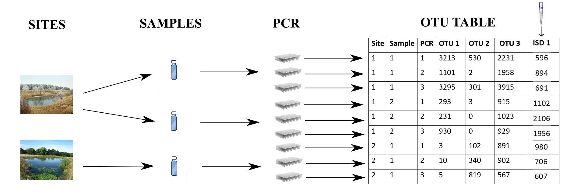
In Stage 2, the physical samples are assayed in the lab. The most frequently used method for reading DNA barcodes from eDNA samples is ‘amplicon sequencing’ (see Lindahl et al.,, 2013, for an excellent review). In short, from each sample, all DNA is extracted and purified. After extraction, a small aliquot of DNA from each sample is subjected to Polymerase Chain Reaction (PCR), which selectively amplifies (makes many copies of) just the DNA-barcode sequences. It is common practice in Stage 2 for a sample to be PCR-assayed multiple times, known as technical replicates to distinguish them from sample replicates in Stage 1. The PCR outputs (‘amplicons’) from all the samples and their technical replicates are pooled and read on a high-throughput DNA sequencer. This procedure ultimately leads to a list of many millions of individual DNA sequences (known as reads), which are processed in a bioinformatic pipeline that removes low-quality reads, then groups the remainder into clusters of similar reads that are species hypotheses known as OTUs (Operational Taxonomic Units), and apportions each OTU’s reads back to its original samples and PCRs. The resulting OTU table dataset indicates the number of reads for each OTU in each PCR in each sample in each site (Figure 1). For simplicity, we hereafter use the terms OTUs and species interchangeably.
A real-world complication in DNA-based laboratory pipelines is that samples are typically ‘normalised’ one or more times. For instance, after the samples are enzymatically digested to break down cells and release their DNA into their ‘lysis-buffer’ solutions, each sample constitutes a larger volume of liquid than can be used for DNA extraction. The samples are thus normalised by taking a fixed volume from each sample for processing. Another normalisation step happens after PCR, because different PCR replicates can generate different amounts of product. In this case, the PCR products are normalised, by taking a certain amount of liquid from each PCR output, either inversely proportional to their concentration, or fixed across PCRs. In the first example, the numerator (amount of lysis buffer taken for extraction) is fixed, while the denominator (total volume of lysis buffer) varies. In the second, the numerator (amount of PCR liquid taken for sequencing) varies, while the denominator (total volume of PCR liquid) is fixed. It is standard procedure to record these normalisation fractions, and in Section 2, we show how this information is incorporated into the model.
Generally, we should expect a positive relationship between the biomass of a species in a sample and the count of reads obtained for that species in that sample (Luo et al.,, 2022), but this relationship is imperfect, due to noise and error (see Table 1). First, even given best practice, there are small but non-negligible probabilities (a) that a species’ DNA in a sample fails to be amplified or sequenced, leading to false-negative error and (b) that a species’ DNA cross-contaminates other samples and is amplified, leading to false-positive error (Stage 2 false negative and false positive error, jointly referred to as Stage 2 error). We say that a PCR yields non-negligible reads for a species when the PCR product of that species is successfully read by the DNA sequencer (i.e. the PCR is successful), and otherwise, a PCR yields non-zero but negligible reads, in which case we say that the PCR is not successful for that species. We note that a PCR can be successful, that is, yield non-negligible reads, not only when the biomass is present in the sample but also when it is not, in the latter case because of contamination. Additionally, PCR amplification also inevitably favours some species over others, due to PCR primer mismatch, resulting in species-specific amplification rates (Stage 2 species effect, equal across rows of the OTU table), and PCR and sequencing stochasticity results in different total numbers of reads across all species, even for the same sample (Stage 2 pipeline effect, equal across columns of the OTU table). Finally, also due to the inherent stochasticity of the PCR and sequencing process, in addition to the species and pipeline effects, there is added noise in the resulting reads in each cell of the OTU table (Stage 2 noise).
In Stage 2, different approaches are employed to understand and monitor some of the noise and error. One such approach is the so-called internal standard or spike-in, during which a known amount of DNA of a synthetic sequence or of a species that is known to be absent from all surveyed sites, is added to each sample. In addition, negative controls, which are samples that are known to not include DNA of any species, can be introduced in Stage 1 and Stage 2 (Ficetola et al.,, 2015; Goldberg et al.,, 2016).
| Stage 1 - biomass collection | |
| Species effect | Every sample contains a certain amount of DNA biomass of each species, with the amount proportional to the biomass available at the site. However, the proportionality constant is unknown and species-specific, since the DNA of different species can be collected at different rates. |
| Noise | The amount of biomass collected for each species varies stochastically between samples collected at the same site. |
| Error | It is possible for the DNA of a target species that is present at a site not to be sampled (false negative error), or traces of DNA from one sample to contaminate another sample (false positive error). |
| Stage 2 - biomass analysis | |
| Species effect | As a result of differences in gene copy number, DNA extraction efficiency, and PCR amplification efficiency, the correspondence between the source sample biomass and the number of amplicon reads is species-specific (column of the OTU table). |
| Pipeline effect | PCR stochasticity and the passing of small aliquots of liquid along the laboratory pipeline affects the total number of reads per technical replicate for all species (row of the OTU table). |
| Noise | In addition to the species and pipeline effect, there is added noise in the number of reads per OTU and PCR (each cell of the OTU table). |
| Error | It is possible for the DNA of a target species that is present in the sample not to be amplified in the lab (false negative error), or traces of DNA of one sample to contaminate and be detected in other samples (false positive error), due to the high species-detection power of amplicon sequencing. |
1.2 Existing approaches
A common approach for modelling metabarcoding data is to convert them to presence/absence data by thresholding the number of reads in the OTU table, with user-specified criteria. This allows the use of a generalized linear model (GLM) framework (Saine et al.,, 2020), which has also been extended to account for species correlation, for example using joint species distribution models (JSDMs) (Ovaskainen and Abrego,, 2020). However, this approach does not account for the two stages or the noise and error inherent in DNA-based surveys (Table 1).
To that end, several different but related approaches have been proposed. A common approach applies occupancy models that account for false negative observation error to the binary presence/absence data (Ficetola et al.,, 2015). More recently, multi-scale extensions of these occupancy models have been proposed to account for false negative error in both stages (Mordecai et al.,, 2011; Schmidt et al.,, 2013) and for false positive error (Guillera-Arroita et al.,, 2017; Griffin et al.,, 2020) for a single species. However, the occupancy model framework disregards the information in the reads and relies on arbitrary thresholds about what constitutes a zero read. Alternatively, the reads have also been modelled within a GLM framework (Takahara et al.,, 2012; Carraro et al.,, 2018) but without considering the errors in each stage. A joint model of species occupancy and corresponding reads was developed by Fukaya et al., (2022) but without considering the direct link between species biomass at the site and species reads, or the correlation between species.
Finally, we note that an area of research similar to DNA-based biodiversity surveys is microbiome biology, which is the genetic material of all microbial life in an abiotic substrate (e.g. soil) or in a living host (e.g. the human microbiome). When modelling microbiome data, interest usually lies in understanding changes in the relative composition of each taxon across different samples. As a result, modelling approaches in this field have revolved around the Dirichlet-Multinomial, which allows inference of the changes, across samples, of the proportions of the species biomasses, but not changes in absolute biomass within each species across samples (Fordyce et al.,, 2011; Coblentz et al.,, 2017; McLaren et al.,, 2019; Clausen and Willis,, 2022). A more detailed comparison between the model we introduce in this paper and models for microbiome data is given in section 2.1.
1.3 Structure of the paper
In this paper, we present a unifying hierarchical modelling framework for OTU reads that considers all key sources of variation, noise, and error at both stages of DNA-based biodiversity surveys (Table 1), while also modelling correlation between species and between sites. The model allows us to infer within-species changes in species biomass across surveyed sites and to link these changes to site-specific covariates.
We use state-of-the-art MCMC (Markov chain Monte Carlo) methods that build on recent work for hierarchical and crossed-effects models (Zanella and Roberts,, 2021) as well as adaptive MCMC techniques (Andrieu and Thoms,, 2008). In particular, we develop a novel sampling technique to improve mixing in the special case of a multivariate crossed-effect model with PCR-specific random effects, and we use adaptive updates of latent variables to focus sampling effort. This allows us to fit our model (with many latent variables across the different stages of DNA surveys) to data from large numbers of sites, samples per site, PCRs per sample, and species.
The new model, its properties, and links to existing models are presented in Section 2. Details on our approach to inference are given in Section 3. Issues of study design are explored and corresponding simulations are presented in Section 4. A case study of a large Malaise-trap metabarcoding dataset is presented in Section 5, and the paper closes with a discussion in Section 6.
2 Model
We assume that physical samples are collected from site , , and PCR replicates are performed on the -th sample from site . We denote by the number of DNA reads of the -th species, in the -th PCR replicate of the -th sample collected at the -th site. We have site covariates and represents their value at site and sample covariates, represented as for the sample at the -th site. In what follows, indexes sites, samples, PCR replicates, and species.
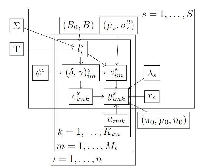
Our proposed model (see Figure 2) is hierarchical, with three levels. The first level models the amount of DNA biomass of each species at the surveyed sites, which is a function of environmental and landscape covariates as well as between-species and between-sites correlation (Biomass availability). The second level models the amount of biomass collected for each species in each physical sample from each site (Biomass collection). Lastly, the third level models the number of reads obtained for each species in each PCR from each physical sample (Biomass analysis). Data are observed only at the third level, as the result of Stage 2 of the survey, with levels one and two corresponding to latent states.
Biomass availability
Biomass collection
|
Biomass analysis
Biomass availability We denote the logarithm of the amount of biomass of species in site available for collection by and denote the matrix by . We model biomass correlation between species and spatial correlation between sites by assuming that follows a matrix normal distribution, (Dawid,, 1981), where is an matrix with columns , with a species-specific intercept, is a design matrix whose rows are , is an matrix of regression coefficients, is an matrix modelling the correlation across sites, and is an matrix modelling the correlation across species. We note that, within this framework, the amount of biomass of a species at the surveyed site cannot be exactly , but can be negligible for modelling purposes as we describe below. We employ a graphical horseshoe (GH) prior (Li et al.,, 2019) for the inverse species covariance matrix , which has the following form
where represents the half-Cauchy distribution (Gelman,, 2006) and . Unlike Li et al., (2019) who specified a flat prior , we follow Wang, (2012) and define a proper prior, ensuring that , which is latent, has a proper posterior. The spatial correlation matrix can be modelled from a kernel function, , such as an exponential kernel, so that , where and are the locations of site and , respectively.
Biomass collection We denote by the amount of biomass of species collected in sample from site and . To account for Stage 1 false negative error at this stage, we introduce latent variable that is equal to if biomass for species has been collected in the -th physical sample from site , and otherwise. We assume that with probability , which is a function of covariates , and of , since higher amounts of biomass are expected to lead to a higher probability of collecting biomass in the sample, leading to . We note that as tends to , tends to , and therefore the species becomes practically impossible to detect. If the amount of biomass collected is greater than 0 (), we model , where models Stage 1 species effects on the biomass collection rate and models the species-specific Stage 1 noise in the biomass collection rate. To account for Stage 1 false positive error, we introduce latent variable , which is equal to 1 with probability if the collected biomass is the result of contamination and otherwise. We assume that can be only if and that if . In this way, we assume that a sample which already contains biomass of a species cannot be further contaminated by the DNA of the same species from another sample or site. We make this assumptions as there is not enough information in the data to partition the collected biomass between that which was truly collected from the site and that which was contamination from elsewhere.
Biomass analysis As mentioned above, by non-negligible reads we mean that some of the PCR product is successfully read by the DNA sequencer. We introduce latent variable to model the success of PCR , sample and site for species , i.e. Stage 2 error. Firstly, if sample from site contains biomass of species (), PCR run can be successful (true positive) , , or not successful (false negative), , and we assume that with probability . Secondly, if sample from site does not contain biomass of species (), PCR run can be successful if it yields non-negligible reads due to lab contamination (false positive), , or not successful (again, , true negative) and assume that with probability .
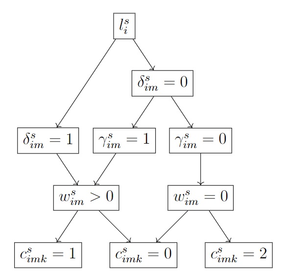
We model the reads conditional on as follows. Conditional on , , where models the Stage 2 species effect on the amplification rate, is the Stage 2 pipeline effect, with , is an offset modeling the normalisation steps described in Section 1.1, and is a species-specific variance of the Stage 2 noise. If more than one normalisation steps are employed, then they can all be incorporated into the same offset i.e. they can be added up. Conditional on , , that is, there are zero reads with probability , and non-zero but negligible reads otherwise. Finally, conditional on , . The negative binomial is parameterised in terms of the mean and the number of failures. A visual representation of the PCR process when is shown in Figure of the Supplementary material.
Stage 2 negative control samples (which are known to not contain DNA of any species) can be easily accounted for in our model by having additional samples for which . Accounting for spike-ins corresponds to having additional species for which ( is known. Since the pipeline effect is shared across all species (including spike-ins), the known values of for the spike-ins help to better estimate . We further investigate this effect in Section 4.
The model is summarised in Figure 2 (a), the directed acyclic graph of the model is shown in Figure 2 (b), while a graphical representation of the latent variables introduced across both stages is shown in Figure 2 (c).
The model presented in Figure 2 is not identifiable in its general form unless certain constraints are applied, as we discuss below. For example, if we define and the model for and conditional on and all offsets set to can be expressed as
| (1) |
It is evident that the model is invariant to transformations of the form
The reason for this unidentifiability is that data are observed only in the third level of the model, and hence the following sets of species-specific parameters are confounded: the baseline amount of biomass across all sites () with the baseline collection rate () and the baseline amplification rate (), and the former again with the baseline detection rate . However, by assuming that all these baseline rates are constant across sites, samples, and PCRs, we are able to infer species-specific changes in biomass across sites and therefore covariate effects and correlations between species and between sites.
For inferential purposes, we set and . Using these constraints, the new baseline (log) amount of biomass, , is equal to , which means that we can only estimate the sum of the baseline amount of available biomass and corresponding baseline collection. Similarly, the new baseline (logit) collection probability is equal to , and therefore the baseline collection probability is also confounded with the baseline collection rate. As a result, we cannot infer the amount of available biomass separately from the collection rate, and hence the estimates of log biomass obtained, as mentioned above, are only meaningful for comparison within each species. For the same reason, comparisons of absolute amount of biomass across species are not meaningful.
We also note that depending on the survey design in terms of the number of samples collected per site and the number of PCR replicates per sample, additional sets of parameters can be confounded and not estimable. Specifically, the following pairs of parameters are confounded:
-
•
: pipeline effect and PCR variance ,
-
•
: PCR variance and the sample noise ,
-
•
: sample noise and site noise .
These are pathological cases that do not involve replication at the site/sample/PCR levels. Replication is vital for being able to account for and to estimate the effects of the different sources of noise and error (Buxton et al.,, 2021), an issue to which we return in Section 4.1.
Finally, we note that if the offsets introduced in the model due to the several normalizations occurring in the pipeline are not recorded, estimates from the model would be biased. However, a potential way to mitigate this bias is the introduction of spike-ins, which contribute to the estimation of the “overall” pipeline effects .
2.1 Special cases
Two models available in the literature arise as special cases of our model (Section 1.2). First, the Dirichlet-Multinomial model (DMM) (Fordyce et al.,, 2011) is expressed through the following hierarchy (omitting the indexes and to simplify notation):
| (2) |
where . The DMM can be seen as a special case of the model described in Section 2, for the Stage process, conditional on . Specifically, , and therefore, assuming , if , the distribution for converges to a . Conditional on , the model is a , where . Next, assuming , we obtain . Finally, as the DMM does not take errors into account, the equivalence with our model can be obtained by setting .
McLaren et al., (2019) propose to account for the Stage 2 species effect in the DMM framework by modelling the probabilities as , where models the species-specific efficiencies, which in our model is achieved by using a species-specific . The DMM can be extended hierarchically if nested treatments are considered (Coblentz et al.,, 2017) by defining a nested prior for each level. In our model, this is achieved by a hierarchy of normal priors. This highlights a key difference between the DMM approach and the approach we introduce in this paper, since we model the propagation of the absolute amount of DNA across the different stages, while the DMM models the propagation of the relative amount of DNA.
Secondly, the occupancy model of Griffin et al., (2020), in the simple case of no covariates,
| (3) |
designed for (single-species) qPCR, can be seen as a special case of the model in Section 2 when the information in the counts is not considered. Specifically, letting be binary, with , and defining , we obtain and . Hence, the model for and becomes
which is identical to the Griffin et al., (2020) model after defining and .
3 Inference
Samples can be drawn from the posterior distribution of the parameters using a Gibbs sampler. Posterior sampling is greatly helped by representing the negative binomial distribution as a Poisson-gamma mixture, which allows many parameters to be updated in closed form from their full conditional distribution.
For the parameters , , and , the full conditional distribution is available in closed form, and therefore posterior sampling is straightforward. We use simple random walk Metropolis Hastings steps for parameters , , , and and Metropolis-Hastings steps with a Laplace approximation proposal for the parameters , , , and . However, on its own, this naive Gibbs sampler will mix slowly since we have a complex hierarchical model with cross effects and many latent variables. We address this by updating parameters in blocks using re-parameterisation and an adaptive updating scheme for the discrete latent variables.
To illustrate our approach to blocking and re-parameterisation, we consider the error-free version of our model
| (4) |
A naive Gibbs sampler updating each parameter from its full conditional leads to prohibitively slow mixing, due to the form of the likelihood where , and appear as a sum. To address the slow mixing in the nested effects, and , the use of a centred parameterisation (Papaspiliopoulos et al.,, 2007) has been suggested, which corresponds to defining and . However, issues of slow mixing still exist between and and, as noted by Zanella and Roberts, (2021), re-parameterisation does not improve mixing in the case of crossed-effects models. In a classic crossed-effect model of the form , Papaspiliopoulos et al., (2020) propose a collapsed Gibbs sampler by first jointly sampling with and then jointly with . However, this approach does not scale well in our setup, since it would involve sampling all the and jointly, which have dimensions and respectively. Zanella and Roberts, (2021) propose the use of identifiability constraints on the model, which in Equation ((4)) correspond to assuming . Since sampling conditionally on constraints can be challenging, we propose a simpler strategy to improve mixing that is more suited to our framework. We consider re-parameterising to the factor averages and and the factor increments and and performing an update by first sampling jointly the factor means conditional on the increments, that is, from and next using the standard updates and . In our simulations, we have found that jointly updating the factor means considerably improves mixing. The sampling scheme for the complete model is presented in the Supplementary material.
The indicator variables can be updated directly from their full conditional distributions but, since there are ) (where is the average number of PCR replicates) of these variables and often one value of has probability very close to , evaluating every full conditional distribution in every iteration can be very time-consuming and computationally wasteful. Therefore, we use a cheap approximation as a proposal in an MH step. Specifically, every iterations, we update the approximation , where is the value of at the t- iteration, is the indicator function which takes the value 1 if is true and 0 otherwise, and is the number of current iterations. Using this update scheme, we only need to evaluate the likelihood if the state is proposed to change. If the probability of one state is close to one, the adaptive scheme often proposes the current state, which can be accepted without computation. The adaptive scheme does not affect convergence of the MCMC algorithm since the approximation clearly has diminishing adaptation and the state space of the indicator variables is discrete (see e.g. Roberts and Rosenthal,, 2009, for more discussion of conditions for convergence of adaptive MCMC schemes).
4 Study design
In this section, we investigate the properties of the model under different study designs in terms of the number of sites, samples per site, and PCRs per sample, as well as the number of spike-ins. In each section, we consider the estimates of the differences in log-biomass within species, when that is not a function of site-specific covariates (no covariate case), and the estimates of the covariate coefficients when log-biomass is a function of a single continuous covariate (regression case).
In Section 4.1 we present theoretical results using a continuous version of our model that does not account for error in either stage. In Section 4.2 we fit our model as presented in Section 2 under different scenarios for study design by varying the number of sites, number of samples per site, and number of PCRs per sample. Finally, in Section 4.3, we explore the effect of spike-ins for different levels of noise in each stage of the process and different study designs.
4.1 Theoretical results
We consider a normal approximation of the model presented in Section 2, which assumes no species or sites correlation, that both stages are error-free by setting , and that the variances of the distributions of the noise at each stage are the same across species. As mentioned in Section 2, the use of spike-ins corresponds to the presence of species in the sample for which ( is known. We assume, without loss of generality, that for . We have the following proposition.
Proposition 4.1.
Consider the model
Then
| (5) |
If we assume that
and , we obtain
| (6) |
Here models the variance of the noise in Stage , as was the case for in the original model. In the no covariate case we have assumed a flat prior on , while in the regression case, we have assumed a single covariate. Equations (5) and (6) show the contribution of the variance of each stage to the posterior variance of the corresponding estimates (changes in species log-biomass between sites and covariate coefficients, respectively) in this special case.
The results for this special case suggest that, for both and , increasing replication at a given stage decreases the contribution of the error variance at that stage and at all downstream stages. For example, increasing the number of samples per site, , reduces the contribution of the noise variances at Stage 1, , and of all downstream stages, i.e. and in Stage 2. Whereas, increasing the number of PCR replicates, , only reduces the contribution of the Stage 2 variances ( and ).
Additionally, the benefit of the spike-in is greater as the ratio of variances increases. Moreover, in the case of , if , the benefit of the spike-in is negligible, as the noise induced by greatly outweighs the noise that can be mitigated via the use of spike-ins.
4.2 Varying , , and
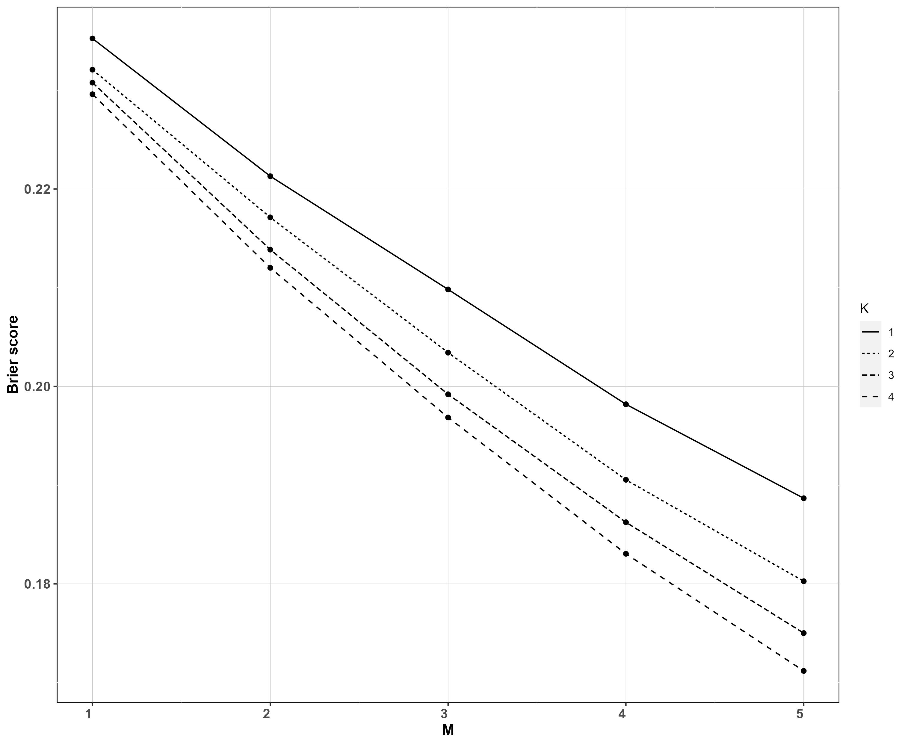
We turn our attention to the full model in Section 2 and again consider the no covariate and regression cases. In the no covariate case, we consider the model’s ability to estimate the correct sign of the difference of species log-biomasses at two sites. We use the Brier score , where is the posterior probability of and is if the true value of is greater than the true value of and otherwise. We separate the sites between those with “high” biomass and those with “low” biomass and generate We use species, sites, samples per site and PCR replicates. The values of the other parameters are reported in the Supplementary Material. We have performed a set of simulations for each combination of values of the design parameters, and . We report the average spanning across the sites with low biomass, across the sites with high biomass, and across all species and across the simulations. As expected, the Brier score decreases, and hence the ability to distinguish between sites with low and high biomass increases, as and increase (Figure 3). However, when , increasing yields little benefit, once more highlighting the greater importance of multiple sample replicates per site in Stage 1, whereas the benefit of larger increases as gets larger.
In the regression case, we consider the absolute error and posterior standard deviation of the covariate coefficient . We use sites, samples per site and PCR replicates per sample and species. The values of the other parameters are reported in the Supplementary Material. We performed a set of simulations for each combination of values of the design parameters and averaged results across all simulations and species, which are shown in Figure 4.
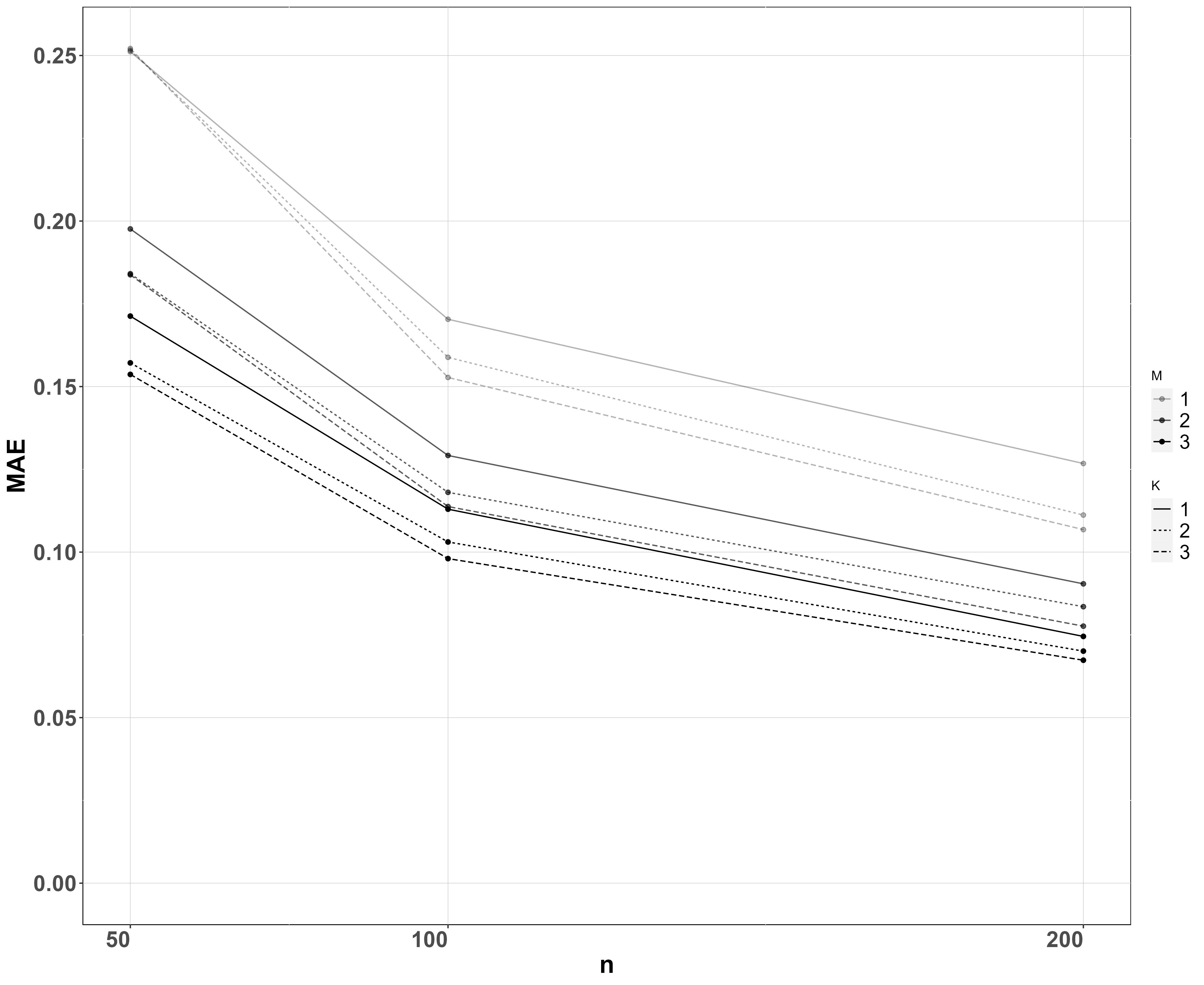
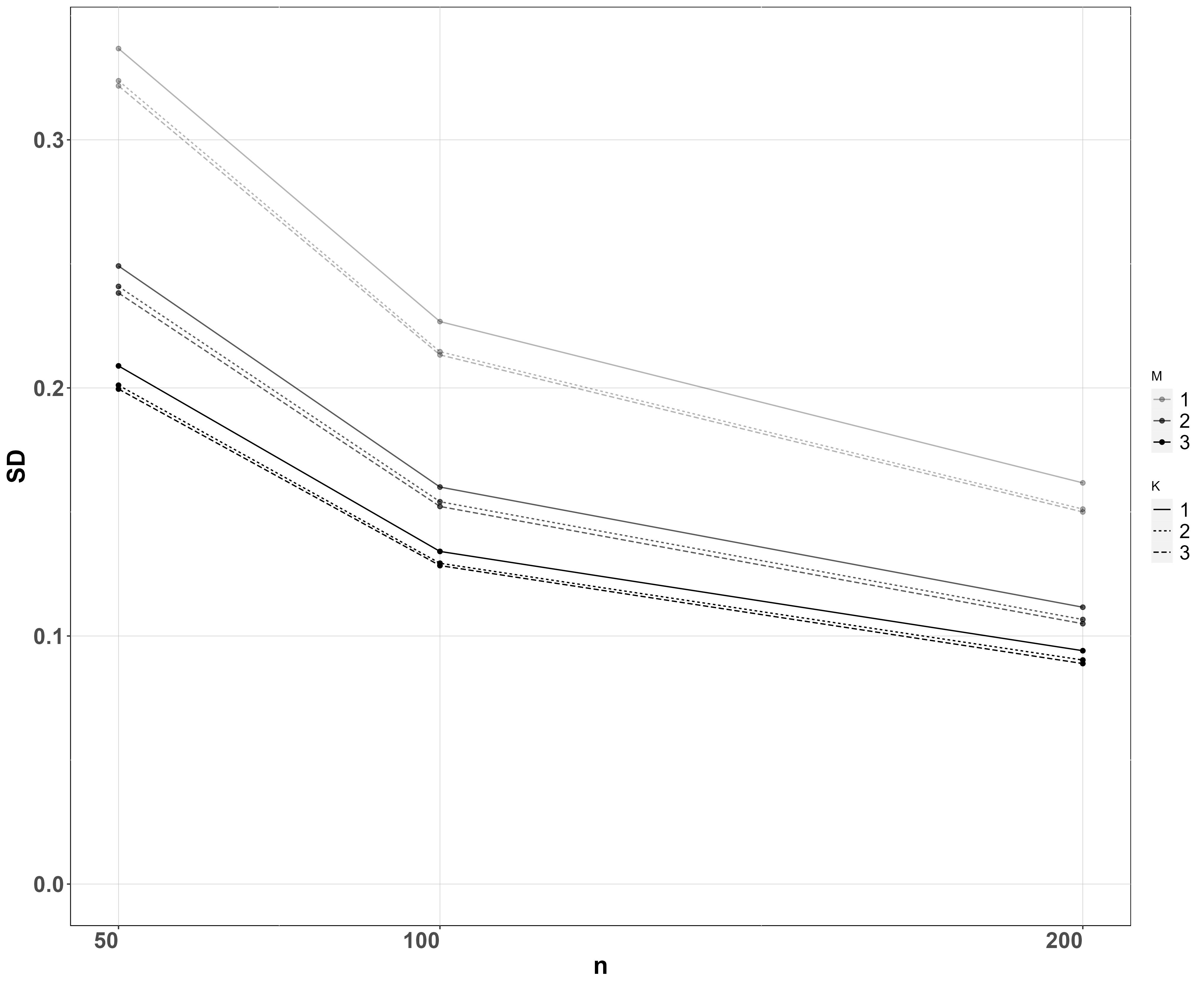
As expected, absolute error and posterior standard error both decrease with more sites , samples per site , and PCRs per sample . Doubling the number of sites from 50 to 100 has a bigger effect than doubling them again from 100 to 200, suggesting that the benefit of increasing the number of sampled sites decreases as the number of sites gets large. Collecting two samples per site instead of one drastically decreases both absolute error and posterior standard deviation, whereas the effect is less pronounced when the number of samples is further increased to three compared to two, while the same can be said about the number of PCRs.
4.3 Spike-ins
In this section, we consider the improvement in inference when spike-ins are employed in Stage 2. We consider a version of the model that does not account for false negative/positive errors, as the effect of the spike-ins is maximised in this case. If errors are present in either or both stages, the benefit of the spike-ins is lower, and dependent upon the level of error.
No covariate
Regression
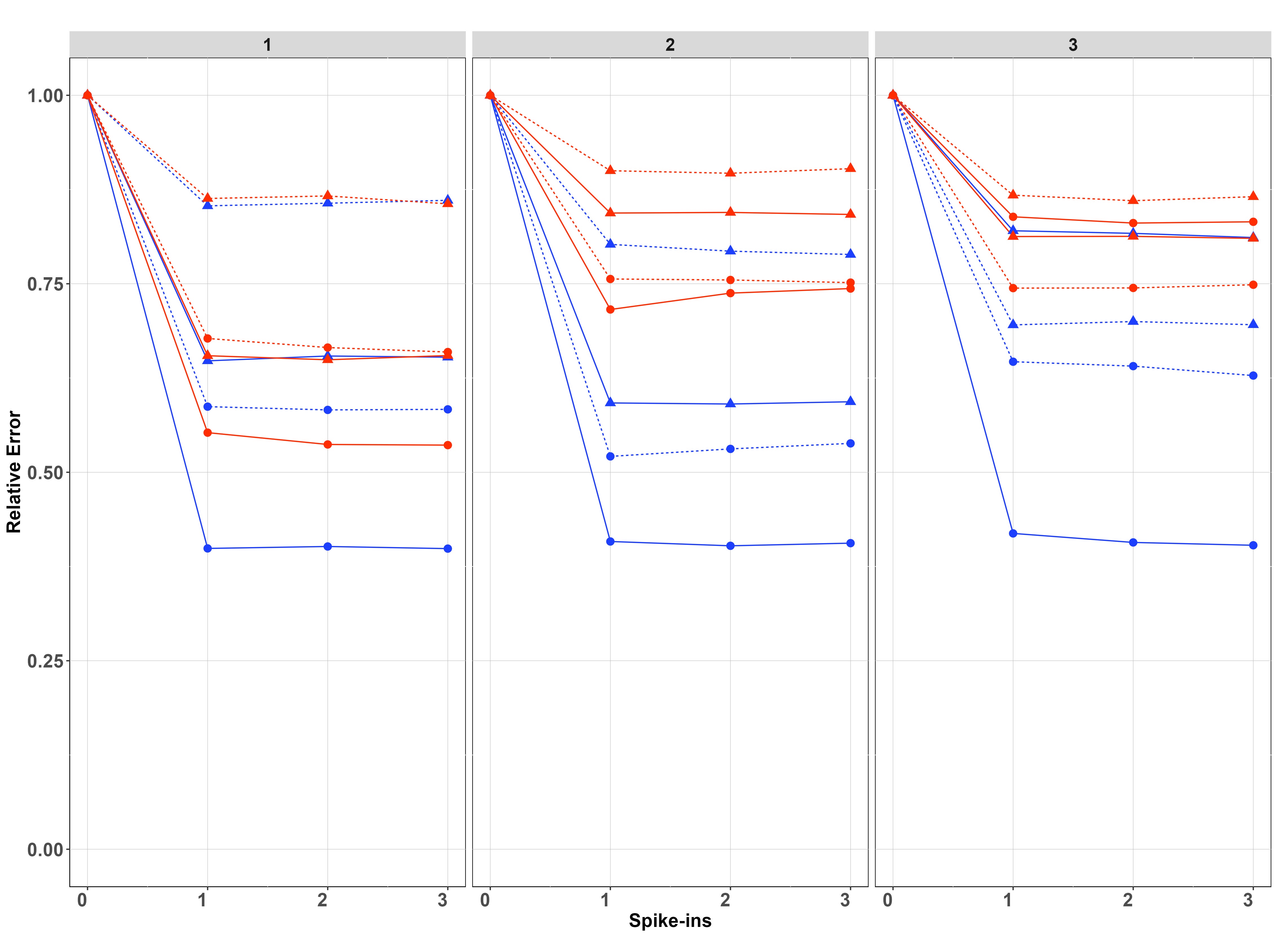
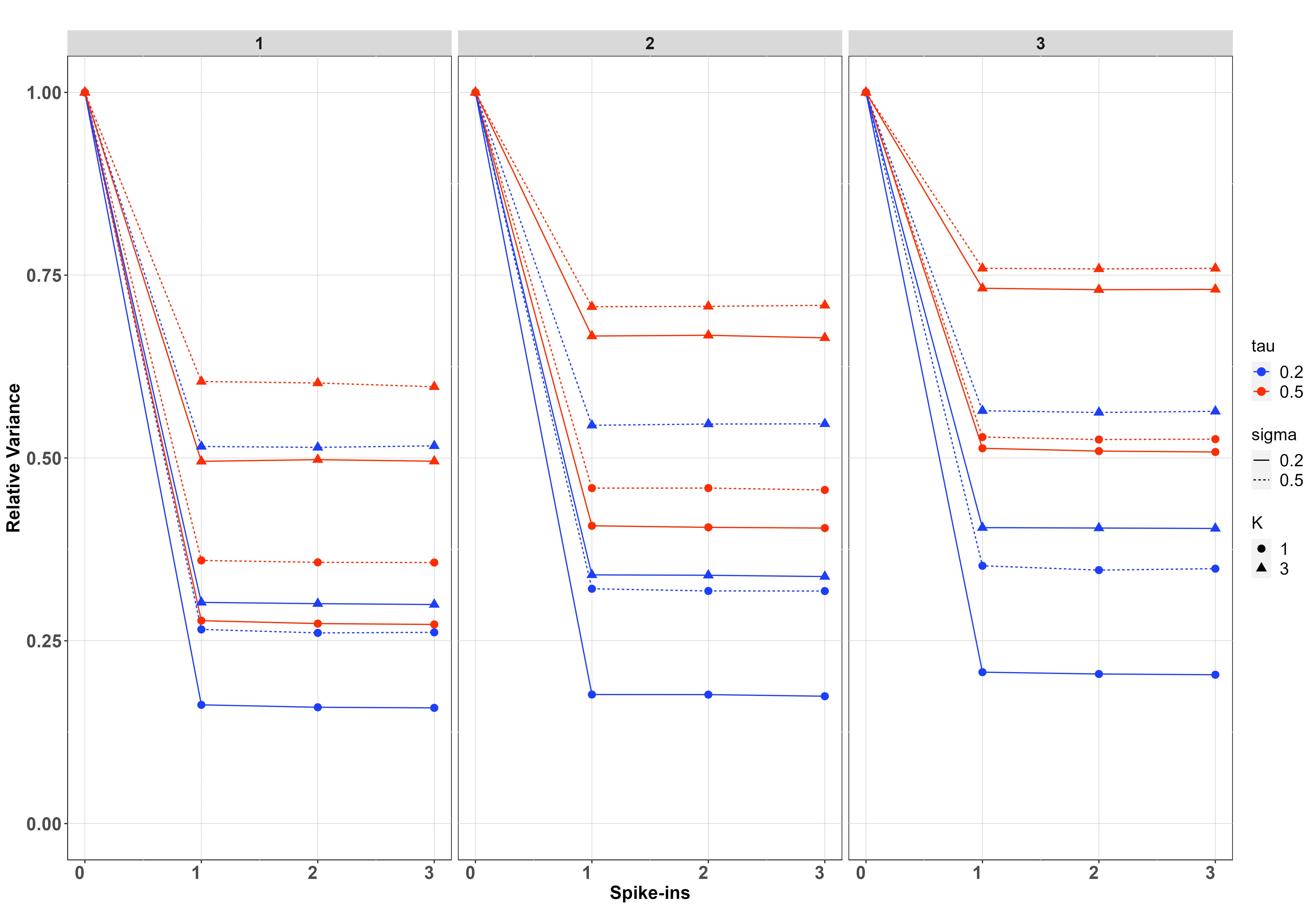
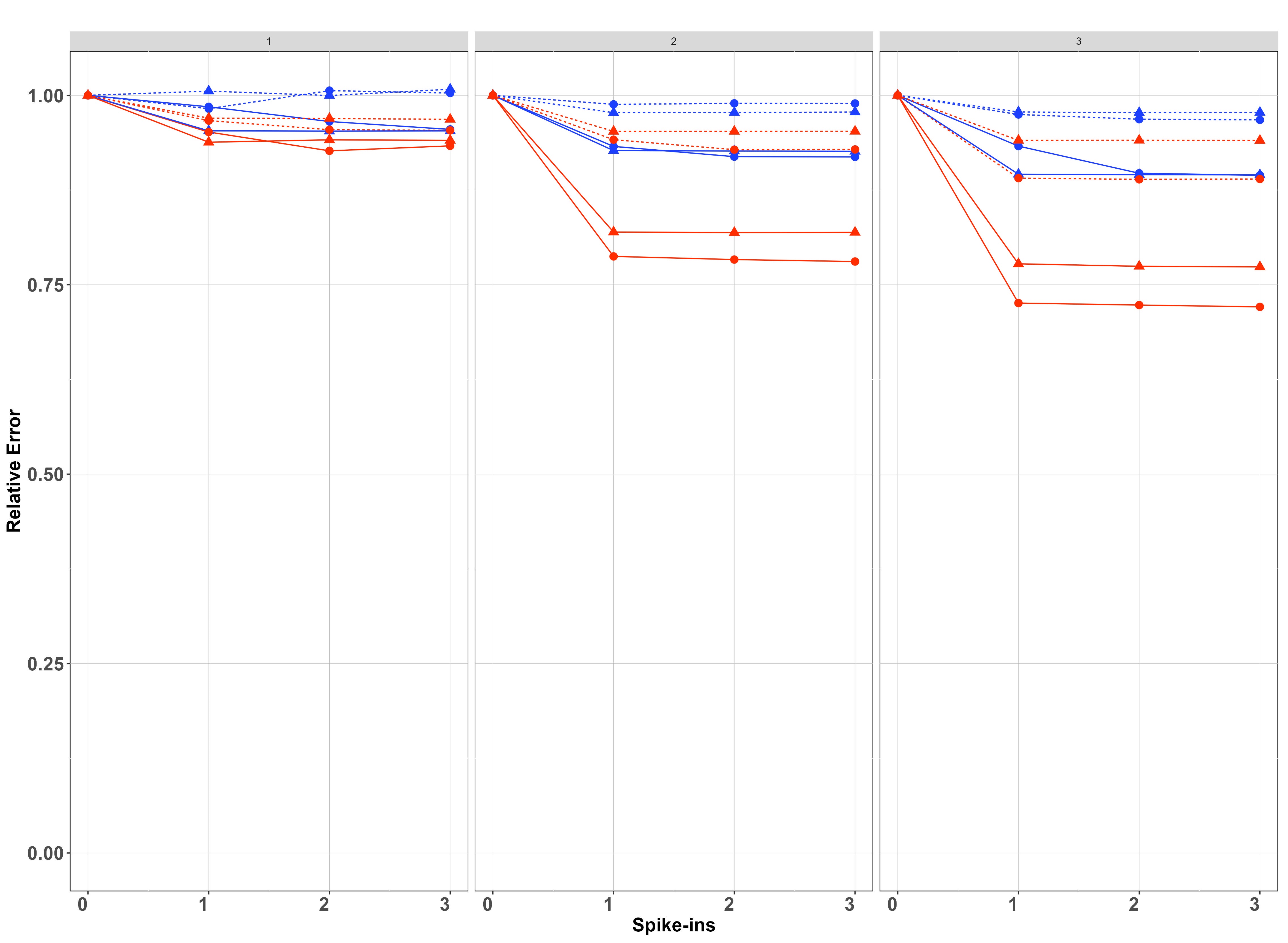
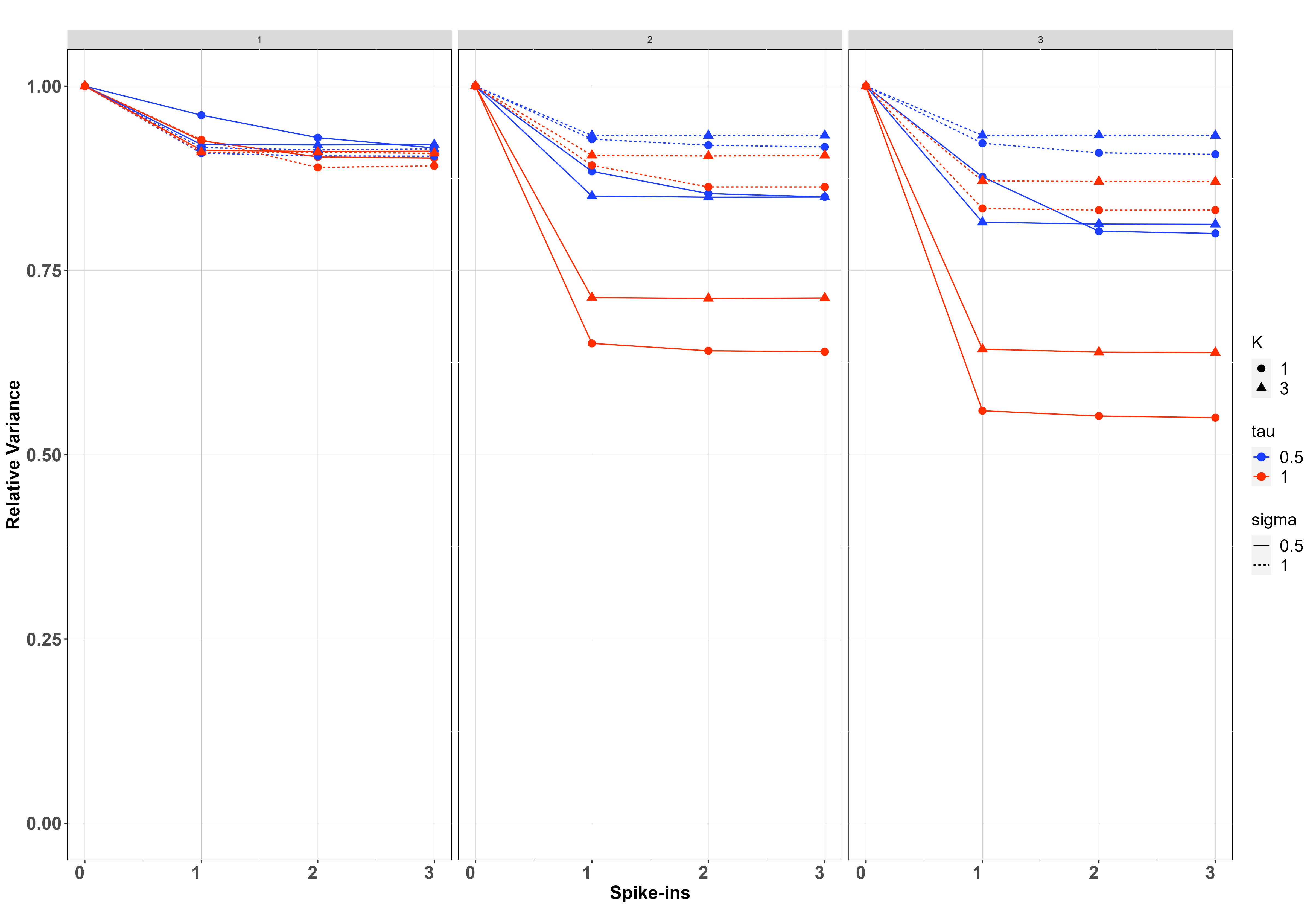
We simulated data on sites, samples per site and PCR replicates per sample on species. For each setting of and , we have fitted the model when and report in each case the posterior relative error and posterior relative variance of the estimates, which are calculated by dividing the posterior error/variance by the corresponding error/variance when using (which is the case with the greatest error/variance).
Results of the simulation study are presented in Figure 5. In both cases, improvements diminish for , and in most cases already provides most of the improvement, suggesting that the benefit of more than one spike-ins is minimal. The no covariate case is shown in the first row of Figure 5. Spike-ins contribute more to reducing biomass-change estimation error and variance with , with resulting in virtually no improvements for any setting considered in the simulation. When , improvement is more pronounced when instead of , because in the latter case, thanks to the replication at Stage 2, there is already increased information for estimating the pipeline effect. This is particularly true when is instead of , because in this case, the differences between sites are more pronounced. For both values of , improvements are bigger when the between-samples standard deviation () is smaller, since otherwise, Stage 1 noise dominates the process and understanding noise in Stage 2 decreases the overall variance proportionally less.
The second row of Figure 5 shows the regression case. We have chosen smaller values for and ( and ), since the relative contribution of the spike-ins is negligible with larger values. Spike-ins contribute more to reducing error and variance when the between-samples standard deviation () and the between-sites standard deviation () is smaller since, similar to before, the noise at early stages dominates the process, and therefore the relative contribution of the spike-ins is smaller due to the improved estimation of the PCR noise. In a similar way to the no covariate case, the contribution of the spike-ins increases for PCR replicates compared to . However, unlike that case, the contribution does not appear to increase as the number of samples per site gets larger.
5 Case study
We apply our model to an unpublished dataset of mostly arthropod invertebrates collected using Malaise-trap samples from sample sites in the H. J. Andrews Experimental Forest (HJA), Oregon USA (225 km2) in July 2018. Each trap was left to collect for seven days, and samples were transferred to fresh 100% ethanol to store at room temperature until extraction. The management objective that motivated the collection of this dataset is to interpolate continuous species distributions among the sample points so that areas of higher and lower conservation value at the HJA can be identified.
For each sample, the collected invertebrate biomass was combined with a lysis buffer, in an amount proportional to the starting biomass, to digest the tissue, and a fixed aliquot was then taken from the overall mixture for DNA extraction and subsequent PCR. This normalization, as described in Section 2, was accounted for in the model by setting the offset equal to the log ratio between the aliquot and the overall amount of liquid mixture in each case.
We included species in the study by selecting the species that have the most non-zero counts across all PCR replicates. Log-biomass is modelled as a function of two environmental covariates: log elevation and log distance-to-road.
Figure 6 presents the 95% posterior credible intervals (PCIs) for the species-specific coefficients of log elevation and log distance-to-road in the model for log-biomass. The effects of the covariates on species biomass are not consistent within each taxonomic order, which suggests low phylogenetic inertia at this rank for response to these landscape characteristics. Elevation is a stronger predictor for species biomass than distance-to-road for this ecosystem. This makes ecological sense, since distance-to-road is only expected to exert an effect over a ca. hundred metres, via canopy openness, whereas elevation exerts a pervasive effect via its effects on temperature, precipitation, and vegetation.
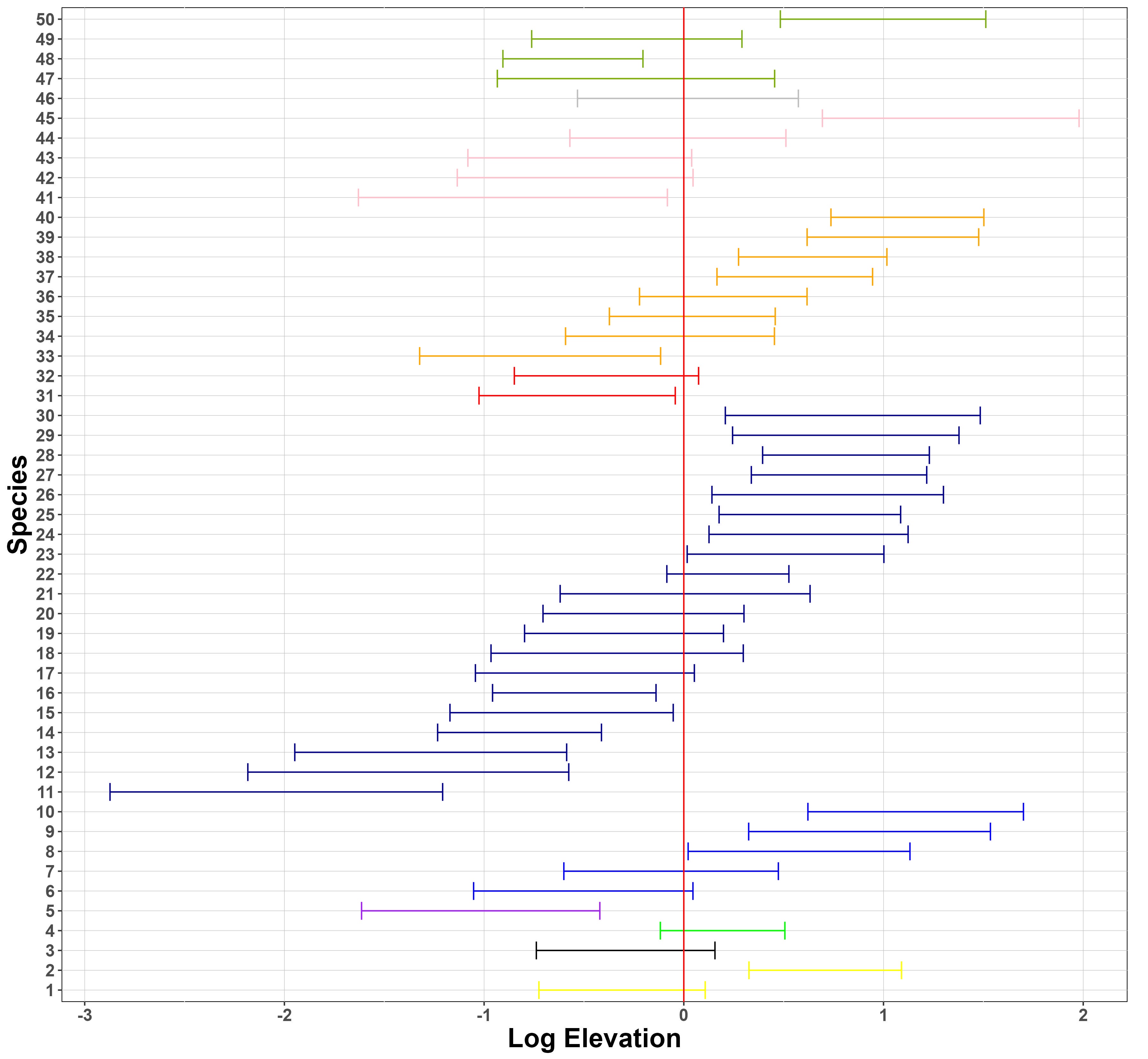
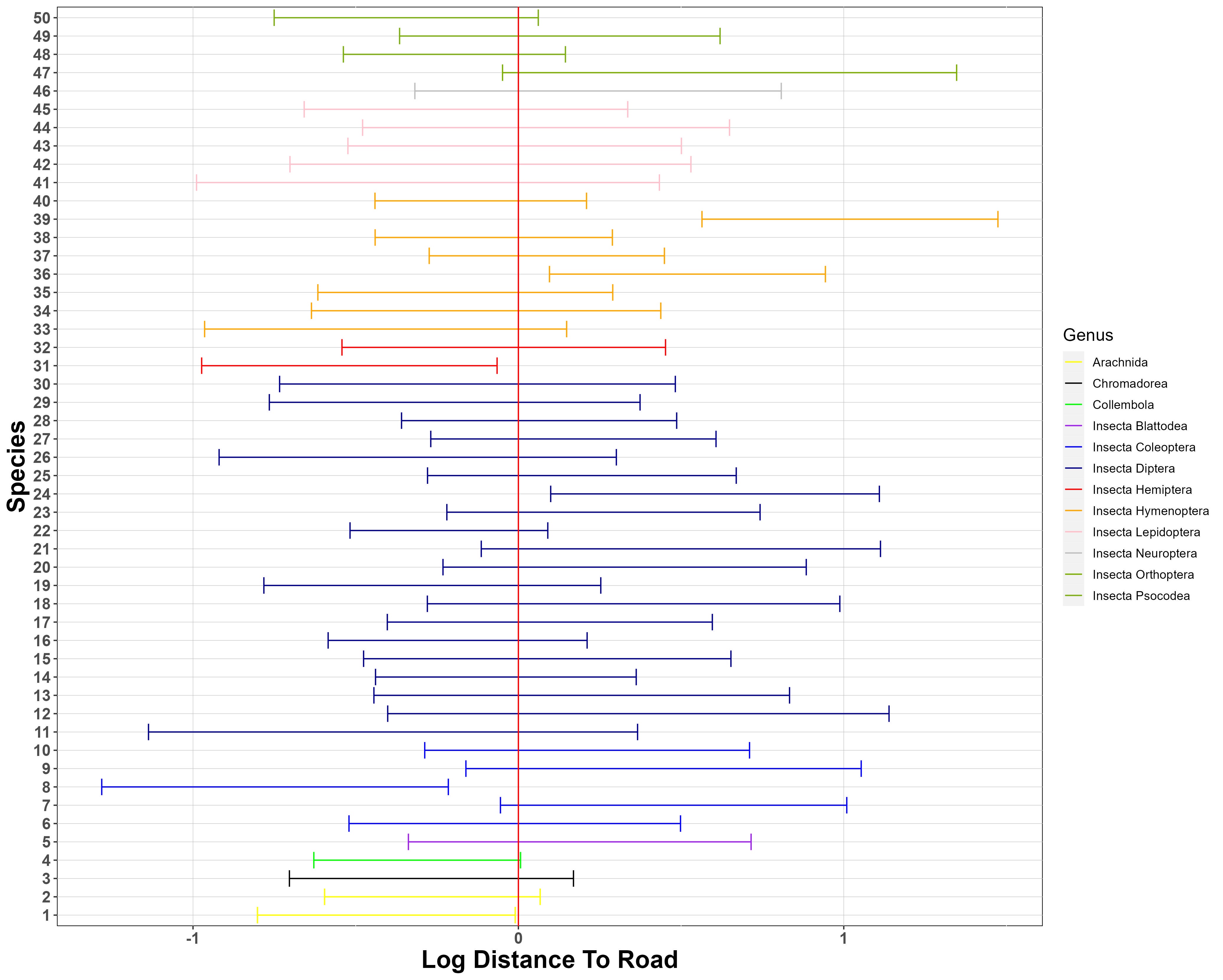
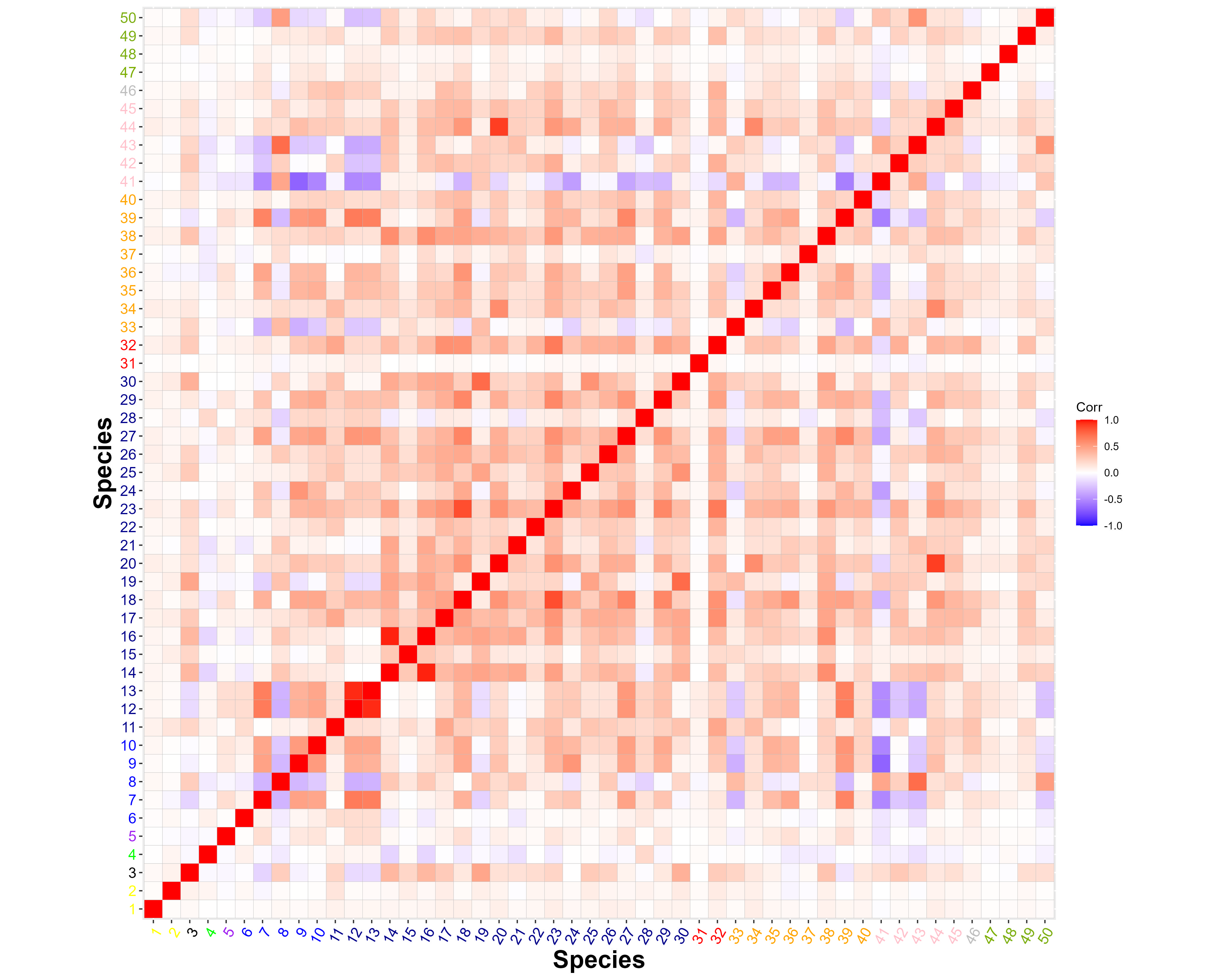
Figure 7 (a) presents the posterior mean of the between-species residual correlations. Species in the Diptera (flies, spp. 14-30) exhibit higher positive correlations with each other, as well as with several species in the Hymenoptera (ants, bees, and wasps) and Lepidoptera (butterflies and months). We conservatively interpret these positive residual correlations as indicative of unmeasured environmental covariates, such as canopy openness, rather than of biotic interactions. We also note that two species in the Lepidoptera, (spp. 41, 43), one in the Hymenoptera (sp. 33), and one in the Psocodea (barklice, sp. 50) are among the few species showing strong negative residual correlation with many of the other species, and again, we interpret these correlations as indicative of unmeasured environmental covariates. There is a strongly positive, pairwise correlation between two tabanid fly species Hybomitra liorhina and Hybomitra sp. indet (spp. 12, 13), which might indicate the oversplitting of one biological species into two OTUs during the bioinformatic pipeline. Finally, there is also a strongly positive, pairwise correlation between the moth species Ceratodelia gueneata (sp. 44) and the predatory fly (Scathophagidae, Microprosopa sp. indet, sp. 20), which might indeed indicate a specialised predator-prey relationship.
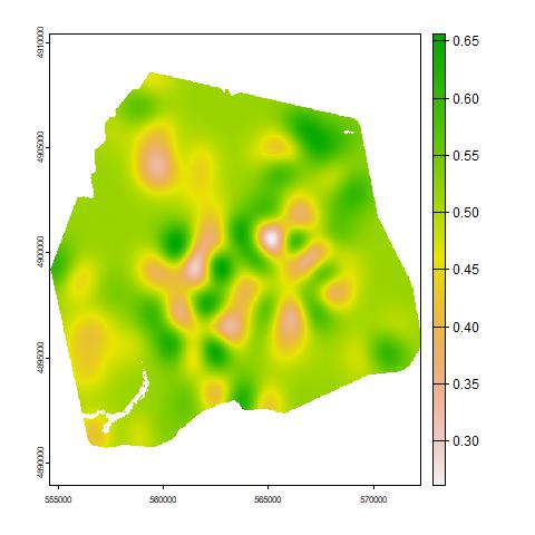
In Figure 7 (b) we show the biodiversity map for the area, which is useful for identifying areas of higher species richness and compositional distinctiveness, which together can be used to identify areas of higher conservation value (i.e. higher ‘site irreplaceability’ sensu Baisero et al.,, 2022). The predicted mean log-biomasses on a continuous map over the HJA for all individual species are presented in the Supplementary Material. These can be used to identify species with a wide spatial range, such as the click beetle (Megapenthes caprella), or with a restricted range, such as the leafhopper (Osbornellus borealis).
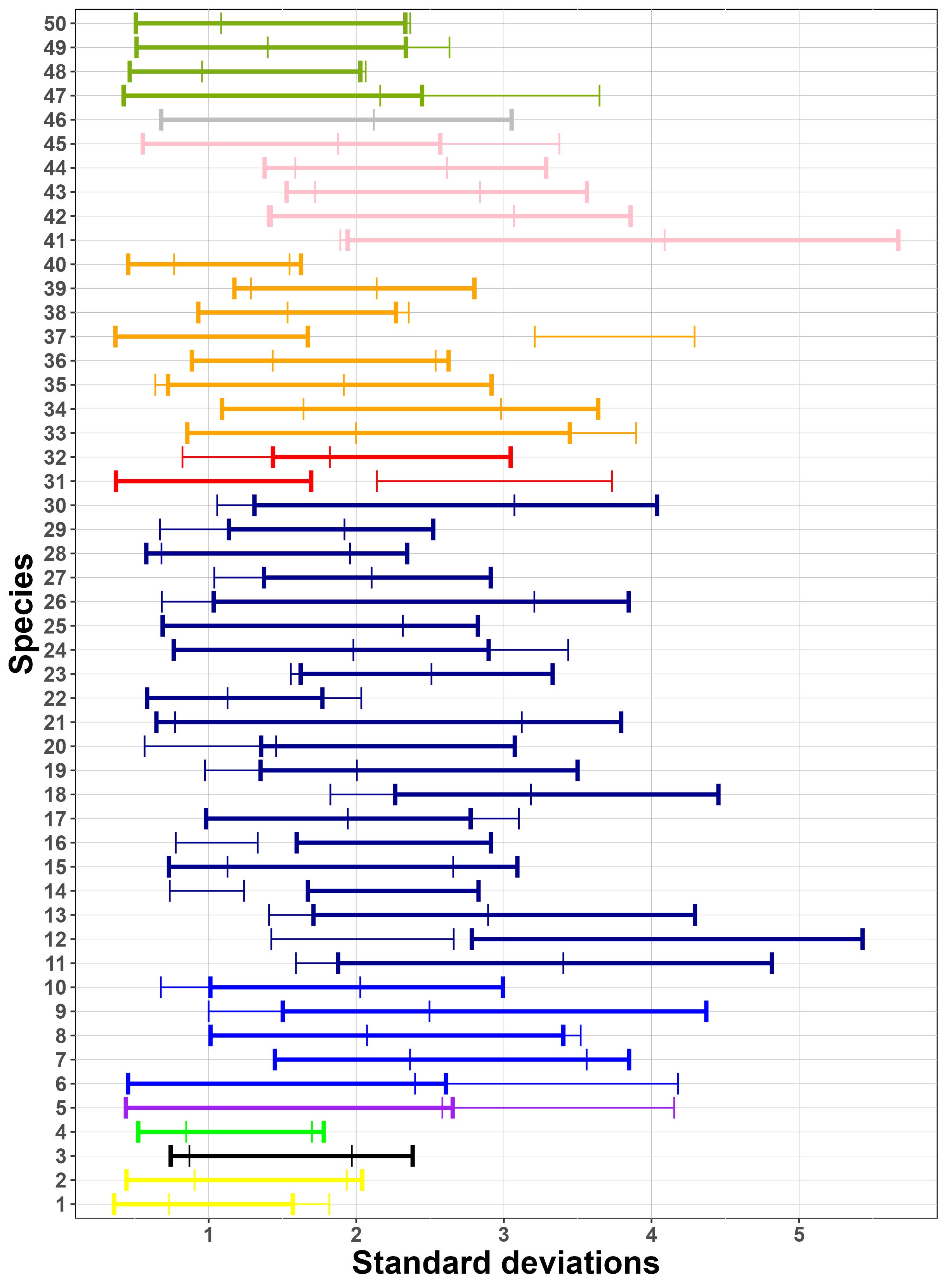
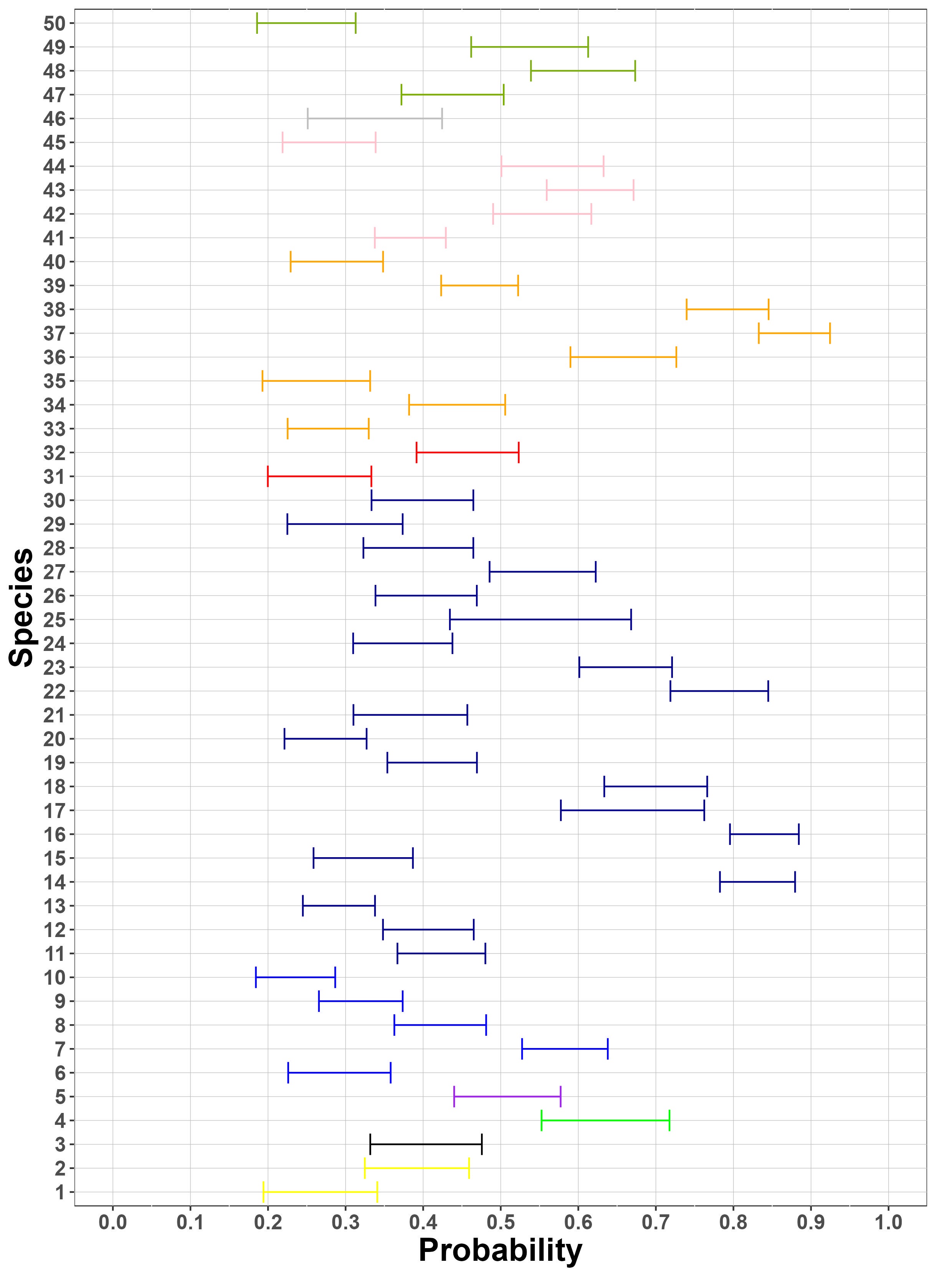
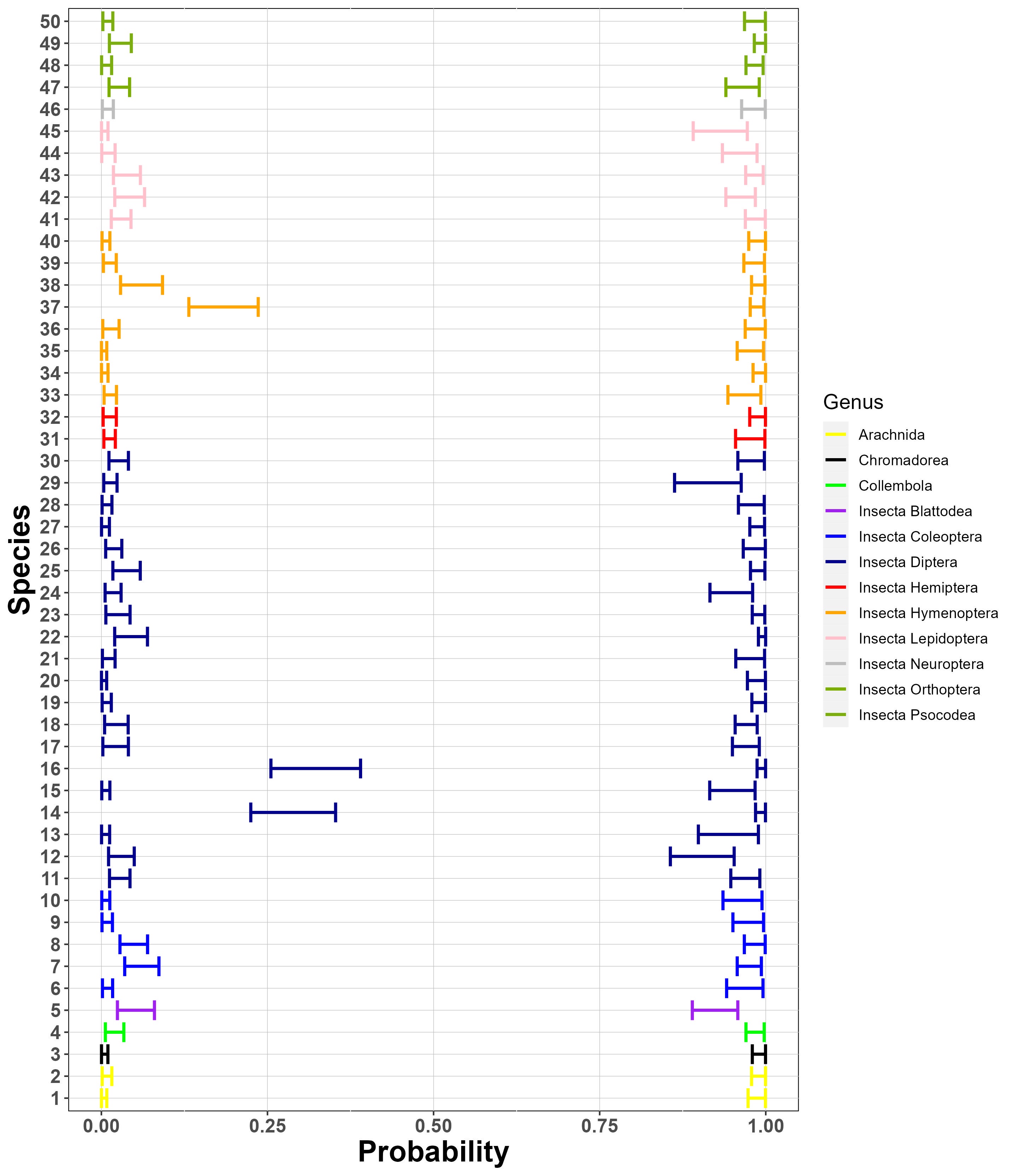
Finally, Figure 8 (a) suggests that generally, there is a similar amount of variation between sites and between samples for these species. As suggested by Figure 8 (b), the species considered have similar collection probabilities across the several sites, possibly due to the fact that the most frequently detected species across PCRs have been selected. Figure 8 (c) demonstrates, as expected, that the Stage 2 true positive probability is close to 1 for all species. Similarly, the figure also suggests that the probability of a Stage 2 false negative error is very close to 0 for all but three species. One of these three (sp. 14) is in the fly family Tachinidae, which are parasitoids of other insects and thus might have been collected not only as adults but also occasionally as eggs attached to the adults of other (insect) host species, with the latter case being classified as false positives in Stage 2, given that an egg would contribute very low amounts of starting DNA biomass.
6 Discussion
Over the last decade, DNA-based biodiversity studies, primarily using metabarcoding, have rapidly increased in popularity, and multivariate statistical models are now starting to be deployed to analyse metabarcoding data (e.g. Lin et al.,, 2021; Pichler and Hartig,, 2020; Abrego et al.,, 2021; Fukaya et al.,, 2022; Ji et al.,, 2022). Our paper provides the first unifying modelling framework that considers and quantifies all main sources of variation, error and noise in metabarcoding surveys (Table 1). As a result, our modelling framework should allow more reliable and more powerful biodiversity monitoring and inference on species responses to landscape characteristics than has been possible before. We have employed, extended, and developed a number of inferential tools to deal with the complexity of the proposed hierarchical model, which involves two latent stages and a large number of latent variables. Finally, this is the first modelling approach that accounts for spike-ins and negative controls (empty tubes), which are widely used quality-control methods in DNA-based biodiversity surveys but rarely explicitly considered within a modelling framework. We explored the benefits of spike-ins on inference and, for the first time, explored issues of study design in metabarcoding data, providing both theoretical and simulation results.
Our new framework allows us to infer and map species biomass as well as biodiversity across surveyed sites (Figure 7 (b)), and to link these to landscape characteristics (Figure 6). The resulting maps can be used to identify areas of high conservation value, as well as areas where particular species or groups of species are more or less prevalent, and to detect species-specific shifts, expansions, and shrinkage. We are also able to study pairwise correlations across large numbers of species (Figure 7 (a)), which is considerably more scalable using metabarcoding data than using standard observational data. We have shown that using spike-ins can substantially increase inference accuracy for parameters of interest (Figure 5). Our results also demonstrate that the current practice of collecting a single sample from each surveyed site considerably reduces our ability to infer changes in species biomass and that replication at both stages as well as the use of spike-ins is the optimal approach to designing metabarcoding studies (Figure 3).
In metabarcoding data, the baseline biomass of each species is confounded with its species-specific collection and amplification rates. Hence, we cannot infer absolute values of species-specific biomass across sites using metabarcoding data alone. However, by assuming that baseline species-specific collection and amplification rates are the same across sites, samples, and PCR replicates, we can infer species-specific biomass change across sites, species-specific covariate effects, and pairwise species correlations. These assumptions are justifiable in the case study, where eDNA release rates cannot differ across sites because the samples are whole organisms, and there is also no reason to believe that Malaise traps vary in trapping efficiency across sites. In other scenarios, eDNA release or degradation rates could vary across the environment, due to large variations in, for instance, food availability and water pH, respectively. In these cases, site covariates could be used to account for this suspected variation.
Generally, modelling changes in (proxies of) abundance, such as changes in biomass, is a more powerful monitoring tool than modelling changes in species presence across surveys sites (Joseph et al.,, 2006). Metabarcoding studies yield count data without any consequence on associated cost, and hence overcome the time and cost implications associated with collecting count data for multiple species. Our model uses the raw count data, and does not rely on ad-hoc rules about what constitutes a practically zero count for converting them to binary data, which has been the standard practice thus far (Ovaskainen et al.,, 2017; Bush et al.,, 2020).
The model can easily be extended to account for multiple primers, which essentially introduce different levels in Stage 2, with each level corresponding to a set of primers. For instance, vertebrate eDNA surveys can profitably use two primers (e.g. the 16S mammal and 12S vertebrate primers used in Ji et al.,, 2022), since the two primers together detect the largest set of vertebrates, with overlap. Additionally, our approach can be extended and applied to metagenomic data. In metagenomics, no PCR is employed. Instead, all the DNA in each mixed-species sample is sequenced, and the DNA barcodes (or other taxonomically informative genetic sequences) are discovered bioinformatically.
Metabarcoding studies, particularly when applied to microbiomes and meiofauna (e.g. nematodes, micro-eukaryotes), can detect 10000s of species, which leads to large numbers of latent variables and coefficients in the model. There are several ways that the inferential tools presented here could be further extended to scale to these cases. Firstly, the posterior distribution conditional on the is independent across species. If could be estimated at a first stage then inference across species could be easily parallelized. Secondly, variational Bayes methods could be applied to avoid the use of sampling methods. The choice of variational distribution will be important and can exploit the conditional normality of much of the model. Alternatively, the model could be adapted by assuming that the coefficient matrices such as , have a low-dimensional representation.
The metabarcoding process produces large numbers of different DNA-barcode sequences, which represent not only different species but also within-species genetic diversity and outright errors generated during PCR and sequencing. Currently, these sequences are clustered into species hypotheses as part of the bioinformatic process, following a number of heuristic rules and thresholds (hence, the word ‘operational’ in OTU), but future work could explore building the OTU table during the model-fitting process.
We are not modelling species presence/absence and instead we have focused on modelling biomass on a continuous scale. As a result, we cannot infer whether a species is absent from a particular study site, but instead only if its biomass at given site is practically zero for modelling purposes. We have assumed that a sample which already contains biomass of a species cannot be further contaminated by the DNA of the same species from another sample or site in Stage 1. This is a reasonable but also necessary assumption. Under best practice, contamination in Stage 1 is expected to be relatively rare, and therefore, there is not enough information in the data to partition the collected biomass between that which was truly collected from the site and that which was contamination from elsewhere. If this assumption is violated, then the amount of collected biomass is no longer proportional to the amount of available biomass, and the amount of available biomass at sites where there has been contamination can be overestimated.
eDNA metabarcoding has revolutionised the cost-effectiveness, precision and scale at which biodiversity assessment can be performed. Nevertheless, the multiple stages at which imperfect detection of biomass can occur during the workflow are not insignificant. By facilitating estimates of within-site changes in biomass and covariates while accounting for workflow uncertainties, our modelling framework provides a step-change improvement in the design and analysis of eDNA metabarcoding data.
References
- Abrego et al., (2021) Abrego, N., Roslin, T., Huotari, T., et al. (2021). Accounting for species interactions is necessary for predicting how arctic arthropod communities respond to climate change. Ecography, 44(6):885–896.
- Andrieu and Thoms, (2008) Andrieu, C. and Thoms, J. (2008). A tutorial on adaptive MCMC. Statistics and Computing, 18(4):343–373.
- Baisero et al., (2022) Baisero, D., Schuster, R., and Plumptre, A. J. (2022). Redefining and mapping global irreplaceability. Conservation Biology, 36(2).
- Besson et al., (2022) Besson, M., Alison, J., Bjerge, K., et al. (2022). Towards the fully automated monitoring of ecological communities. Ecological Letters, to appear.
- Bohmann et al., (2014) Bohmann, K., Evans, A., Gilbert, M. T. P., et al. (2014). Environmental DNA for wildlife biology and biodiversity monitoring. Trends in Ecology & Evolution, 29(6):358–367.
- Bush et al., (2020) Bush, A., Monk, W. A., Compson, Z. G., et al. (2020). DNA metabarcoding reveals metacommunity dynamics in a threatened boreal wetland wilderness. Proceedings of the National Academy of Sciences, 117(15):8539–8545.
- Bush et al., (2017) Bush, A., Sollmann, R., Wilting, A., et al. (2017). Connecting Earth observation to high-throughput biodiversity data. Nature Ecology & Evolution, 1(7):0176.
- Buxton et al., (2021) Buxton, A., Matechou, E., Griffin, J., et al. (2021). Optimising sampling and analysis protocols in environmental DNA studies. Scientific Reports, 11(1):11637.
- Carraro et al., (2018) Carraro, L., Hartikainen, H., Jokela, J., et al. (2018). Estimating species distribution and abundance in river networks using environmental DNA. Proceedings of the National Academy of Sciences, 115(46):11724–11729.
- Clare et al., (2022) Clare, E. L., Economou, C. K., Bennett, F. J., and others. (2022). Measuring biodiversity from DNA in the air. Current Biology, 32(3):693–700.e5.
- Clausen and Willis, (2022) Clausen, D. S. and Willis, A. D. (2022). Modeling complex measurement error in microbiome experiments. arXiv preprint arXiv:2204.12733.
- Coblentz et al., (2017) Coblentz, K. E., Rosenblatt, A. E., and Novak, M. (2017). The application of Bayesian hierarchical models to quantify individual diet specialization. Ecology, 98(6):1535–1547.
- Dawid, (1981) Dawid, A. P. (1981). Some matrix-variate distribution theory: notational considerations and a Bayesian application. Biometrika, 68(1):265–274.
- Ficetola et al., (2015) Ficetola, G. F., Pansu, J., Bonin, A., et al. (2015). Replication levels, false presences and the estimation of the presence/absence from eDNA metabarcoding data. Molecular Ecology Resources, 15(3):543–556.
- Fordyce et al., (2011) Fordyce, J. A., Gompert, Z., Forister, M. L., and Nice, C. C. (2011). A hierarchical Bayesian approach to ecological count data: a flexible tool for ecologists. PloS One, 6(11):e26785.
- Frøslev et al., (2019) Frøslev, T. G., Kjøller, R., Bruun, H. H., et al. (2019). Man against machine: Do fungal fruitbodies and eDNA give similar biodiversity assessments across broad environmental gradients? Biological Conservation, 233:201–212.
- Fukaya et al., (2022) Fukaya, K., Kondo, N. I., Matsuzaki, S.-i. S., and Kadoya, T. (2022). Multispecies site occupancy modelling and study design for spatially replicated environmental DNA metabarcoding. Methods in Ecology and Evolution, 13(1):183–193.
- Gelman, (2006) Gelman, A. (2006). Prior distributions for variance parameters in hierarchical models. Bayesian Analysis, 1(3):515–533.
- Goldberg et al., (2016) Goldberg, C. S., Turner, C. R., Deiner, K., et al. (2016). Critical considerations for the application of environmental dna methods to detect aquatic species. Methods in Ecology and Evolution, 7(11):1299––1307.
- Griffin et al., (2020) Griffin, J. E., Matechou, E., Buxton, A. S., et al. (2020). Modelling environmental DNA data; Bayesian variable selection accounting for false positive and false negative errors. Journal of the Royal Statistical Society: Series C (Applied Statistics), 69(2):377–392.
- Guillera-Arroita et al., (2017) Guillera-Arroita, G., Lahoz-Monfort, J., van Rooyen, A., Weeks, A., and Tingley, R. (2017). Dealing with false-positive and false-negative errors about species occurrence at multiple levels. Methods in Ecology and Evolution, 8(9):1081–1091.
- Hebert et al., (2003) Hebert, P. D., Cywinska, A., Ball, S. L., and DeWaard, J. R. (2003). Biological identifications through dna barcodes. Proceedings of the Royal Society of London. Series B: Biological Sciences, 270(1512):313–321.
- Ji et al., (2013) Ji, Y., Ashton, L., Pedley, S. M., et al. (2013). Reliable, verifiable and efficient monitoring of biodiversity via metabarcoding. Ecology Letters, 16(10):1245–1257.
- Ji et al., (2022) Ji, Y., Baker, C. C. M., Popescu, V. D., et al. (2022). Measuring protected-area effectiveness using vertebrate distributions from leech iDNA. Nature Communications, 13(1):1555.
- Joseph et al., (2006) Joseph, L. N., Field, S. A., Wilcox, C., and Possingham, H. P. (2006). Presence–absence versus abundance data for monitoring threatened species. Conservation Biology, 20(6):1679–1687.
- Ley, (2022) Ley, R. (2022). The human microbiome: there is much left to do. Nature, 606(7914):435–435.
- Li et al., (2019) Li, Y., Craig, B. A., and Bhadra, A. (2019). The graphical horseshoe estimator for inverse covariance matrices. Journal of Computational and Graphical Statistics, 28(3):747–757.
- Lin et al., (2021) Lin, M., Simons, A. L., Harrigan, R. J., et al. (2021). Landscape analyses using eDNA metabarcoding and Earth observation predict community biodiversity in California. Ecological Applications, 31(6).
- Lindahl et al., (2013) Lindahl, B. D., Nilsson, R. H., Tedersoo, L., et al. (2013). Fungal community analysis by high-throughput sequencing of amplified markers–a user’s guide. New Phytologist, 199(1):288–299.
- Luo et al., (2022) Luo, M., Ji, Y., Warton, D., and Yu, D. W. (2022). Extracting abundance information from DNA‐based data. Molecular Ecology Resources, to appear.
- Lynggaard et al., (2022) Lynggaard, C., Bertelsen, M. F., Jensen, C. V., et al. (2022). Airborne environmental dna for terrestrial vertebrate community monitoring. Current Biology, 32(3):701–707.e5.
- McLaren et al., (2019) McLaren, M. R., Willis, A. D., and Callahan, B. J. (2019). Consistent and correctable bias in metagenomic sequencing experiments. Elife, 8:e46923.
- Mordecai et al., (2011) Mordecai, R. S., Mattsson, B. J., Tzilkowski, C. J., and Cooper, R. J. (2011). Addressing challenges when studying mobile or episodic species: hierarchical Bayes estimation of occupancy and use. Journal of Applied Ecology, 48(1):56–66.
- Ovaskainen and Abrego, (2020) Ovaskainen, O. and Abrego, N. (2020). Joint Species Distribution Modelling: With Applications in R. Cambridge University Press.
- Ovaskainen et al., (2017) Ovaskainen, O., Tikhonov, G., Dunson, D., et al. (2017). How are species interactions structured in species-rich communities? A new method for analysing time-series data. Proceedings of the Royal Society B: Biological Sciences, 284(1855):20170768.
- Papaspiliopoulos et al., (2007) Papaspiliopoulos, O., Roberts, G. O., and Sköld, M. (2007). A general framework for the parametrization of hierarchical models. Statistical Science, 22(1):59–73.
- Papaspiliopoulos et al., (2020) Papaspiliopoulos, O., Roberts, G. O., and Zanella, G. (2020). Scalable inference for crossed random effects models. Biometrika, 107(1):25–40.
- Pawlowski et al., (2020) Pawlowski, J., Apothéloz‐Perret‐Gentil, L., and Altermatt, F. (2020). Environmental DNA: What’s behind the term? Clarifying the terminology and recommendations for its future use in biomonitoring. Molecular Ecology, 29(22):4258–4264.
- Pichler and Hartig, (2020) Pichler, M. and Hartig, F. (2020). sjSDM: Scalable Joint Species Distribution Modeling.
- Piper et al., (2019) Piper, A. M., Batovska, J., Cogan, N. O. I., et al. (2019). Prospects and challenges of implementing DNA metabarcoding for high-throughput insect surveillance. GigaScience, 8(8):giz092.
- Ratnasingham and Hebert, (2007) Ratnasingham, S. and Hebert, P. D. (2007). Bold: The barcode of life data system (http://www. barcodinglife. org). Molecular Ecology Notes, 7(3):355–364.
- Roberts and Rosenthal, (2009) Roberts, G. O. and Rosenthal, J. S. (2009). Examples of adaptive MCMC. Journal of Computational and Graphical Statistics, 18(2):349–367.
- Saine et al., (2020) Saine, S., Ovaskainen, O., Somervuo, P., and Abrego, N. (2020). Data collected by fruit body-and DNA-based survey methods yield consistent species-to-species association networks in wood-inhabiting fungal communities. Oikos, 129(12):1833–1843.
- Schmidt et al., (2013) Schmidt, B. R., Kery, M., Ursenbacher, S., et al. (2013). Site occupancy models in the analysis of environmental dna presence/absence surveys: a case study of an emerging amphibian pathogen. Methods in Ecology and Evolution, 4(7):646–653.
- Taberlet et al., (2018) Taberlet, P., Bonin, A., Zinger, L., and Coissac, E. (2018). Environmental DNA: for biodiversity research and monitoring. Oxford University Press, Oxford, United Kingdom, first edition edition.
- Takahara et al., (2012) Takahara, T., Minamoto, T., Yamanaka, H., et al. (2012). Estimation of fish biomass using environmental dna. PloS one, 7(4):e35868.
- Thomsen and Sigsgaard, (2019) Thomsen, P. F. and Sigsgaard, E. E. (2019). Environmental DNA metabarcoding of wild flowers reveals diverse communities of terrestrial arthropods. Ecology and Evolution, 9(4):1665–1679.
- Thomsen and Willerslev, (2015) Thomsen, P. F. and Willerslev, E. (2015). Environmental DNA – An emerging tool in conservation for monitoring past and present biodiversity. Biological Conservation, 183:4–18.
- Tosa et al., (2021) Tosa, M. I., Dziedzic, E. H., Appel, C. L., et al. (2021). The Rapid Rise of Next-Generation Natural History. Frontiers in Ecology and Evolution, 9:698131.
- van Klink et al., (2022) van Klink, R., August, T., Bas, Y., et al. (2022). Emerging technologies revolutionise insect ecology and monitoring. Trends in Ecology & Evolution, 37(10):872–885.
- Wang, (2012) Wang, H. (2012). Bayesian graphical lasso models and efficient posterior computation. Bayesian Analysis, 7(4):867–886.
- Zanella and Roberts, (2021) Zanella, G. and Roberts, G. (2021). Multilevel linear models, gibbs samplers and multigrid decompositions (with discussion). Bayesian Analysis, 16(4):1309–1391.