Effect of the Atomic Dipole-Dipole Interaction on the Phase Diagrams of Field-Matter Interactions I: Variational procedure
Abstract
We establish, within the second quantization method, the general dipole-dipole Hamiltonian interaction of a system of -level atoms. The variational energy surface of the -level atoms interacting with -mode fields and under the Van Der Waals forces is calculated with respect the tensorial product of matter and electromagnetic field coherent states. This is used to determine the quantum phase diagram associated to the ground state of the system and quantify the effect of the dipole-dipole Hamiltonian interaction. By considering real induced electric dipole moments, we find the quantum phase transitions for - and -level atomic systems interacting with - and - modes of the electromagnetic field, respectively. The corresponding order of the transitions is established by means of Ehrenfest classification; for some undetermined cases, we propose two procedures: the difference of the expectation value of the Casimir operators of the -level subsystems, and by maximizing the Bures distance between neighbor variational solutions.
I Introduction
Recently, we have studied the quantum phase diagrams of a system of -level atoms interacting with electromagnetic modes in a cavity, under the dipolar aproximation Cordero et al. (2021); López-Peña et al. (2021).
When the inter-atomic distance of a cold atomic gas is comparable to the wavelength of the electromagnetic field, the dipole-dipole coupling between the atoms becomes important and yields relevant collective effects Weiner et al. (1999). These Van der Waals forces, due to dipole-dipole interactions of the induced electric dipole moments, become important and must be taken into account. However, one needs to be careful about the long or short character of the dipolar potential for many particle systems, as one can find in theoretical and experimental studies of ultra-cold boson systems Jones et al. (2006); Lahaye et al. (2009); Astrakharchik and Lozovik (2008).
The dipole-dipole interaction decays as , with the distance between particles, and is thus of a different nature as the matter-field interaction considered in earlier works (cf., e.g., Cordero et al. (2015) and references therein). Energy transfer between the particles (atoms, molecules) is one of the important consequences of this interaction. For Rydberg atoms it is particularly interesting, as they have high principal quantum numbers , while the dipole moment scales as in atomic units Gerry and Knight (2005).
A review of theoretical and experimental work on the dipole-dipole interaction between Bose-Einstein condensates has been presented in Lahaye et al. (2009). The trapping of cooled polar molecules and other atomic species Doyle et al. (2004) was important for attracting the attention to study these type of interactions, and the long-range dipole-dipole interaction in low-density atomic vapors was detected in Yu et al. (2019), confirming that the interaction is indeed long-range, and that it is present at any density.
According to the previous discussion, the interaction between atoms might be relevant to the determination of the quantum phase diagrams for the system constituted by -level atoms interacting with -modes of electromagnetic radiation in a cavity. The main objective of this work is to quantify the effect of the atomic dipole-dipole induced interaction on the properties of the ground state of the system. The original contributions of this work are the following: To establish the general dipole-dipole interaction Hamiltonian for a system of -level atoms interacting with -modes of electromagnetic radiation in a cavity. To calculate the associated energy surface, which allows us to determine the variational ground state, playing a fundamental role in finding the quantum phase diagrams of the system. The cases for - and - level atomic configurations are worked out explicitly, determining the quantum phase diagrams together with the corresponding order of the transitions. It is remarkable that, even for a finite number of atoms, the surface of maximum Bures distance is able to detect the phase transitions where the Ehrenfest method does not. Additionally we have found that the quantum phases continue to be dominated by a set of monochromatic regions as it was the case for noninteracting atoms, at least when the induced electric dipolar moments are real.
The paper is organized as follows: Section II derives the model for a system of identical -level atoms interacting with modes of an electromagnetic field, including the atomic dipole-dipole interaction, and particularizes it for - and -level atoms. Section III constructs the variational energy surface from a complete set of test states which approach the quantum ground state, or any other quantum excited state. Here we focus on the ground state and study its phase diagram. This is applied in section IV to the case of -level atoms, and in section V to the case of -level atoms in their different atomic configurations, finding the critical values of the coupling parameters which minimize the energy, and determining the phase diagram in both attractive and repulsive scenarios of the atomic dipole-dipole interaction. In cases where a phase transition exists which defies the Ehrenfest classification, new criteria are proposed, one based on the second Casimir operator and another one based on the maximum Bures distance between neighboring states. Finally, section VI summarizes some conclusions. Two appendices present the matter collective operators and the atomic dipole-dipole operator in explicit form.
II Model
We consider a system of identical -level atoms interacting with modes of a radiation field, placed in a cavity. The Hamiltonian is composed of three terms
| (1) |
where is the diagonal contribution given by ()
| (2) |
the dipolar matter-field interaction is of the form Cordero et al. (2013)
| (3) |
In these expressions, and are the field frequency and photon number operator, respectively, of mode ; denotes the energy of the -th atomic level with the convention for ); and are the field creation and annihilation operators; and is the atomic transition operator between levels and , which in a bosonic representation plays the role of the collective matter operator obeying the unitary algebra in dimensions, ; here, creates an atom in level and annihilates one in level (cf. Eq. (54). The dipolar matter-field coupling intensity between field mode and atomic dipole formed by levels and is denoted by .
Atoms do not have permanent dipole moments in their ground state, as the center of charge of the electronic cloud coincides with that of the nucleus. In the presence of an electromagnetic field, however, these centers are displaced and the induced transition dipole moments are responsible for an atomic dipole-dipole interaction. In second quantization this dipole-dipole interaction takes the form
| (4) |
where bosonic creation and annihilation operators were used. The factor in eq. (4) compensates the double accounting in the summation, as the particles are indistinguishable. The factor is included to have an interaction linear in the number of particles. The first index in the bra and the ket states corresponds to the first particle, while the second index corresponds to the second particle.
The set of operators that appear in (4) may be rewritten in terms of the collective matter operators, by means the bosonic commutation relation, as
| (5) | |||||
where we have defined the oslash product between collective matter operators, which removes the self-interaction terms (see appendix A for more details).
The dipole-dipole interaction is obtained from the classical expression Jackson (1999) through the standard quantization procedure, which has the form
| (6) |
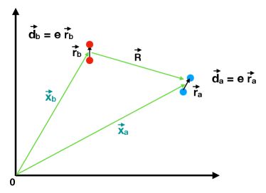
where are the induced vector operators of the electric dipole moments, is the separation between the dipoles and (with ) the unitary vector in the direction from one dipole to another, at positions and (see Fig. 1). is the permittivity of vacuum, and for induced magnetic moments , the expression is the same with the replacements , and , the magnetic permeability of vacuum (cf., e.g., Cohen-Tannoudji et al. (heim)). Without loss of generality, we will consider here that the induced electric dipoles are real.
Thus, the two-body matrix elements in Hilbert space are
| (7) |
The indices of the dipole-dipole coefficient refer to the two dipoles involved in the bra-ket (7).
For indistinguishable particles, and identifying the expansion components of the dipolar operator in terms of the collective matter operators, viz. the dipolar operator given by , the matrix element in Eq. (7) reads
| (8) |
where stands for the average distance between pairs of atoms. The hermiticity of Eq.(4) follows from the relations
| (9) |
Also, for real dipolar vectors , one has .
Finally, using the oslash operator introduced above, we may write the dipole-dipole interaction in a simplified form as
| (10) |
Inserting the different contributions into (10), one may write the atomic dipole-dipole term in the Hamiltonian as (see appendix B)
| (11) |
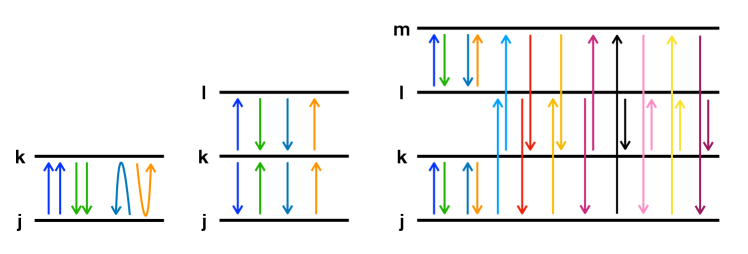
where the operator stands for the dipole-dipole contribution of the pair ; the operator for that of the pair of dipoles (here the atomic level plays the role of an intermediate level, so a prohibited dipolar transition is possible via the permitted dipolar transitions and ); and the operator corresponds to the contribution of isolated dipoles (which do not share an energy level). The upper index denotes the number of different atomic levels which contribute to the interaction; hence, the terms and are zero for -level atoms with and , respectively. The set of transitions included in each interaction term is given in table 1, and shown schematically in figure 2. These terms are given in appendix B. Also, the factors and in expression (11) eliminate the double summation due to index reordering.
| Atomic levels | Interaction | Atomic Transitions | |
|---|---|---|---|
Amongst the parameters in the Hamiltonian, we are free to choose and , i.e., the energies are normalized to the highest atomic level. We also consider systems where only one field mode promotes the transition between a given pair of atomic levels; this constriction is imposed by the condition Cordero et al. (2016)
| (12) |
Since the interaction (11) involves the dipole-dipole contribution , we have only when and for at least one of the modes and . The first and second order Casimir operators [Eqs. (52 and 53)], whose eigenvalues are functions of the number of atoms and the number of levels , are of course constants of motion.
As an example, we now write explicitly the contribution of for two- and three-level atoms:
-level atoms
For a system of two-level atoms, the Hamiltonian (1) reads
| (13) |
where we fix for the atomic levels respectively.
-level atoms
-level atoms present three different atomic configurations (, and ), according to which atomic transitions are prohibited.
-
•
For the -configuration, the dipolar transition is prohibited, and the Hamiltonian takes the form
(14) The intermediate atomic level may promote the transition . The set of nonzero dipolar-dipolar strengths is together with their complex conjugates, obtained as , cf. Eq. (9).
-
•
For the -configuration it is the dipolar transition which is prohibited, and the Hamiltonian takes the form
(15) The atomic level serves as an intermediate level which may promote the transition . The set of nonzero dipolar-dipolar strengths is together with their complex conjugates obtained by Eq. (9).
-
•
For the -configuration the dipolar transition is prohibited, and the Hamiltonian is
(16) The atomic level acts here as an intermediate and may promote the transition . The set of nonzero dipolar-dipolar strengths is together with their complex conjugates obtained by Eq. (9).
In a recent work Civitarese et al. (2010) the case where equal contributions of the form for all , was considered (other terms were neglected). It was shown that the dipole–-dipole interactions act against the appearance of atomic squeezing, and also that an increase in the mean value of the number of photons of the initial state smears out the effect.
III Variational energy surface
The variational solution involves a test state which approaches the quantum ground or desired excited state, and which depends on a set of parameters . The corresponding energy surface is obtained by taking the expectation value of the Hamiltonian and minimizing with respect to the parameters of the test state. In this work we focus on the ground state and take as test state the direct product of coherent states for both the matter and the field contributions. Clearly, this test state presents no matter-field entanglement, but it yields a good description of the minimum energy surface, as well as some expectation values of the physical quantities, and the phase diagram together with the order of the phase transitions.
Coherent matter state
The coherent matter state is defined as Iachello and Arima (1987)
| (17) |
where and . The operator is
| (18) |
and, using the bosonic realization it is immediate that the relationship is fulfilled; hence, the state (17) is normalised. It is straightforward to show that
| (19) |
which for any number of atoms generalizes to
| (20) |
The relations above are useful in order to find the matrix elements of the collective matter operators. The linear contribution is
| (21) |
and the quadratic contribution
| (22) | |||||
where the last term corresponds to the self-interactions, and vanishes in the dipole-dipole interaction.
Coherent field state
The coherent field state for modes is given by the direct product of coherent states for each mode, as follows Klauder and Skagerstam (1985); Ali et al. (2014),
| (23) |
where . For each mode the coherent state satisfies , and hence
| (24) |
while the expectation value of the number operator for each mode is
| (25) |
From the expressions above, and writing for the complete test state the direct product of the coherent states for field and matter,
| (26) |
the variational energy surface per atom , as a function of , , and parameters of the Hamiltonian, reads
| (27) | |||||
where . The last term in (27) corresponds to the atomic dipole-dipole interaction per particle , and has the form
| (28) | |||||
Here, we used the fact that and in order to simplify the expression.
By simple inspection, one may note that the energy surface has minima at the critical values and , with
| (29) |
and .
In a similar fashion, for the fixed values and , and supposing, without loss of generality, real values for the dipolar () and dipole-dipole () strengths, one finds the critical values for the phase to be .
After substitution of the critical values , and fixing and , we obtain a family of energy surfaces for and ; appropriate values for and should be selected in order to satisfy in Eq. (29). The minimum energy surface is then obtained by calculating the critical points , which is done numerically in general.
IV Two-level atoms
For two-level atoms the expression of the energy surface reads
| (30) | |||||
with . The critical values of the corresponding energy surface Eq. (27) must satisfy
| (31) |
and, fixing and , one finds two solutions
| (32) |
Here, we have used a dimensionless matter-field coupling intensity , defined as
| (33) |
with the critical value of the coupling constant when the atomic dipole-dipole interaction is neglected, and where ; we have also defined
| (34) |
to simplify the notation.
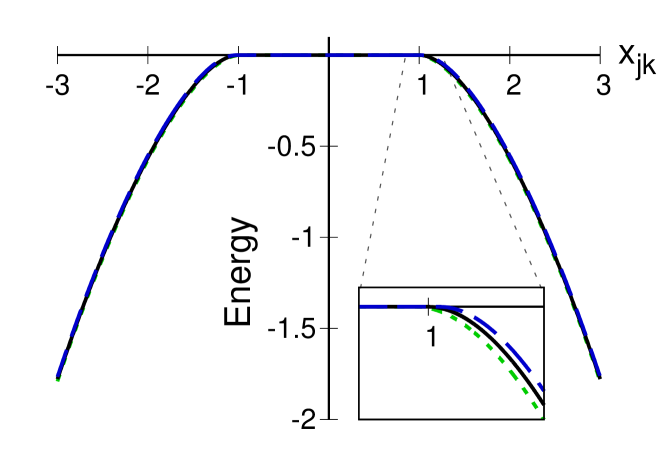
For values one finds only one critical value , for which the energy surface has the constant value . When we have two critical values (32), in this case the energy surface has a dependence on the matter-field dipolar strength . After minimizing one finds
| (35) |
This relationship, vs. , is shown in figure 3. The solid line (black) corresponds to the case without atomic dipole-dipole interaction; repulsive (dashed line, blue) and attractive (dotted line, green) cases are also shown. Due to the minuteness of this interaction when compared with the dipolar matter-field interaction, the difference for dissimilar values of is difficult to appreciate. We have zoomed around the value (see figure inset) where the transition into the collective region appears, in order to make this difference clear. In what follows, we will consider unnaturally large values for the atomic dipole-dipole coupling parameter so that its effect may be appreciated; when studying actual realistic systems these values (and their effects) must be scaled down accordingly.
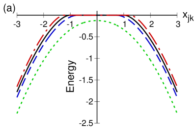
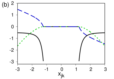
The minimum energy for different (larger) values of the dipolar coupling strength is plotted in figure 4. For values of such that , the critical points divide the normal region from the collective region . One should note that for the case without dipole-dipole interaction, , (solid line in figure 4(a)) the critical points occur at , while in the attractive case (dashed line in figure 4(a)) one has , i.e., the normal region decreases. Correspondingly, for the repulsive case (dot-dash line in figure 4(a)) the normal region increases, as we have . The anomalous behaviour is the strong attractive regime, this is characterised by values of such that , when the normal region vanishes completely (dotted line in Fig. 4(a)). It is important to note that, for large matter-field coupling , the minimum energy surface tends to that without the atomic dipole-dipole interaction; in other words, the effect of the dipole-dipole terms on the energy surface is seen mainly in a vicinity of the normal region.
The order of the transition may be determined using the Ehrenfest classification Gilmore (1993), which involves the derivatives of the energy surface. We exemplify the case in figure 4(b), showing, respectively, the first (dashed-line) and second derivatives (solid line) of the energy. Since the second derivative presents a discontinuity at the critical point , a second order transition occurs at that location.
V Three-level atoms
For three-level atomic systems interacting dipolarly with a two-mode electromagnetic field in a cavity, the atomic dipole-dipole interaction can be obtained from expression (10) or (59). For the case of real induced dipole moments one has only to consider the real coupling strengths for two-level interactions, and for those associated to three-level interactions. Thus the induced dipole-dipole interaction for three-level atoms takes the form,
Notice that for the different atomic configurations one has at most three real parameters; in the case of the configuration, for instance, we have the coupling strengths and .
The corresponding variational energy surface for the dipole-dipole interaction may be obtained by taking the expectation value of (V) with respect the variational state , or from the general expression (28) by considering real induced dipole moments together with three-level atomic systems and a two-mode electromagnetic field. The resulting expressions for the , and atomic configuration are given by
| (37) | |||||
| (38) | |||||
| (39) |
For systems of -level atoms interacting with two modes of electromagnetic field, the critical values of the phases (vide supra) are and , for which the relationship is satisfied, and where we defined . Also, the critical values associated to the field are given as functions of the critical values of the matter [cf. Eq. (29)]. These values must be calculated numerically, except when the dipole-dipole interaction is neglected, since in this latter case we have an analytical solution Cordero et al. (2015).
In this work we calculate the critical values for the three atomic configurations (, and ) and obtain the corresponding separatrix; we fix in all cases the double resonant condition, i.e., the field frequencies are given by and . The atomic levels satisfy the condition with and . We take and the value for the -configuration, and for the -configuration, and and for the -configuration. The values considered for the dipolar-dipolar strength , assuming real dipolar vectors , are given in table 2.
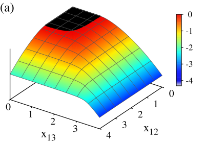
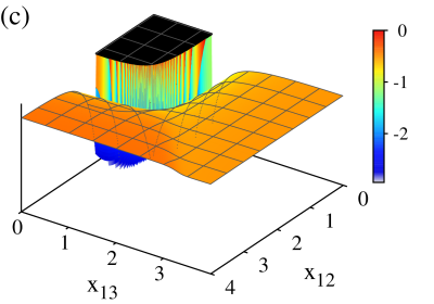
In order to exemplify how to obtain the separatrix, we consider explicitly the particular case of the -configuration with a repulsive dipole-dipole strength . The set of critical points and are evaluated numerically and inserted into the expression for the minimum energy; the result is shown in Fig. 5(a). The normal region, where , is colored in black. The separatrix is found by calculating the first derivatives of the energy surface, as
| (40) |
which is shown in Fig. 5(b). It is a continuous surface. We calculate the second order derivative as
| (41) |
which is discontinuous [cf. Fig. 5(c)]. The loci form a separatrix which splits the normal from the collective region; in fact, this discontinuity shows that a second order transition occurs at these points for the -configuration.
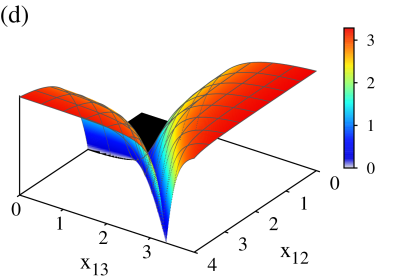
In Fig. 5(c), the slight undulation (observed by a small change in the orange hue of the surface) within the collective region in the second derivative of the minimum energy surface, is a signature of a kind of transition due to a change of subspaces formed by -level atoms, as was discussed recently for the case without dipole-dipole interaction Cordero et al. (2015), from one subspace in which one of the radiation modes dominates to another subspace where the other mode dominates. This change grows as , and gives a discontinuity when . However, for values the second derivative remains continuous, as well as derivatives of higher order; in other words, the Ehrenfest classification does not provide a criterion to determine that the transition exists. In this work, we propose to consider the second order Casimir operator corresponding to each -level subsystem in order to label this transition (vide infra).
The second order Casimir operator for a system of particles of -levels is given by
| (42) |
In particular, when only two levels are considered, we may define
| (43) |
which coincides with the second order Casimir operator for -levels. Therefore, the expectation value will be close to when the bulk of the contribution to the state is given by the basis of the sub-system of the two levels . Since the variational solution is independent of , we fix for this calculation and consider the absolute value of the difference of the second order Casimir operator of each subsystem
| (44) |
where stands for the ground state.
This quantity is plotted in figure 5(d), showing that it is sensitive to the transition in the collective region. The points in the collective region where a transition occurs are given by , indicating that the bulk of the ground state changes from one sub-space to the other.
Another criterion that we have proposed Cordero et al. (2021); López-Peña et al. (2021) in order to find transitions not detectable through the Ehrenfest classification, is to use the Bures distance in the total product space of -level atoms and -mode radiation field, defined by Bures (1969); Uhlmann (1976)
| (45) |
for states
| (46) |
and maximize it for neighboring states. As a general procedure, one selects various points around a circumference of radius about each point in parameter space, in order to find the state with maximum distance to (cf. Cordero et al. (2021); López-Peña et al. (2021) for details). In our case, it was sufficient to calculate it for four points about each in order to get a qualitative behavior of the surface of maximum Bures distance.
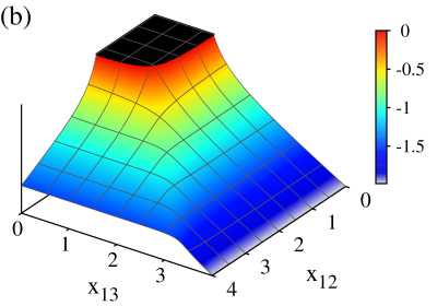
Figure 6 shows, for (a) and for (b), the surface of maximum Bures distance between neighboring states. Note that the transition within the collective regions stands out, and for we reach the maximum distance of for variational states in the thermodynamic limit. We may refer to this as a transition of the kind continuous unstable, in the sense that this transition tends to a first order one in the limit .
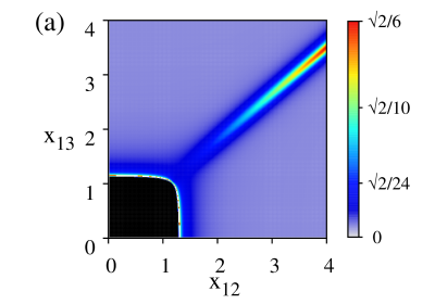
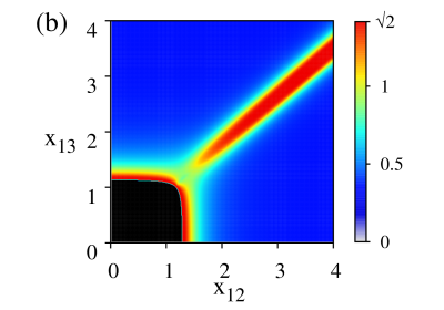
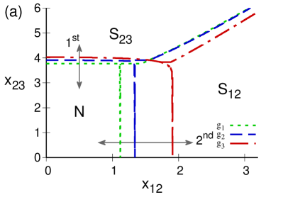
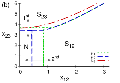
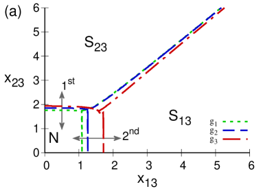
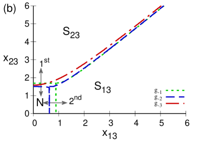
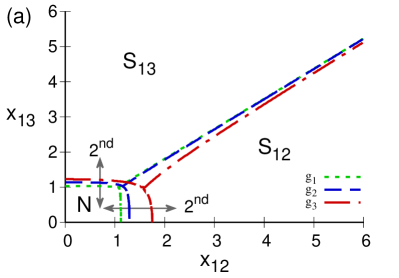
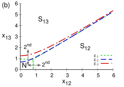
Figure 7 shows the separatrix for the atomic -configuration, in the case of a repulsive dipole-dipole interaction 7(a), and in the case of an attractive one attractive 7(b). One notes that, in the repulsive case, the normal region grows as the dipole-dipole interaction grows. The regions where the bulk of the ground state is dominated by the basis of the subsystem or are also indicated. The order of the phase transitions are marked: a first order transition for and second order transition for . In the attractive case, Fig. 7(b), the normal region decreases in size as increases in magnitude, and it in fact vanishes for the value of where only the regions and subsist; for and the order of the phase transitions is the same as in the repulsive case.
A similar behavior occurs for the -configuration, Fig. 8, where the subregions in the collective regime are and .
Figure 9 shows the situation for atoms in the -configuration. In the repulsive case, Fig 9(a), a normal region exists in all the circumstances, and the transitions from the normal to the collective region are of second order. For the attractive case, Fig 9(b), in the case (dotted line) a normal region exists and we have a second order transition. In the strong attractive cases of and we only have the collective regions and .
VI Conclusions
We have established the general atomic dipole-dipole interaction Hamiltonian for a system of -level atoms interacting with -modes of electromagnetic radiation in a cavity, together with the associated energy surface, which allows to determine the variational ground state (see expressions (27), (28), and (29)). For - and -level atomic configurations, we have found that for attractive (repulsive) atomic dipole-dipole interactions the normal region decreases (increases) in size. The quantum phase diagrams, together with the corresponding order of the transitions, have also been determined. For a finite or infinite number of atoms, the surface of maximum Bures distance is able to detect the transitions between the collective regions where the Ehrenfest criterion fails (see Fig. 6). In other words, we find that, in cases where the Ehrenfest criterion for the phase transitions does not give information, a criterion based on the maximum probability for prohibited transitions comes to the rescue. We have also proved that the quantum phase diagrams continue being dominated by monochromatic regions as it is the case for noninteracting atoms, at least for real induced electric dipolar moments.
Phase diagrams for - and -level atoms interacting with an external radiation field have been studied, for all the possible atomic configurations. It is seen that the atomic dipole-dipole interaction is minuscule compared with the dipolar matter-field interaction, so the atomic dipole-dipole coupling has been exaggerated in order to see its consequences. (The unnaturally large values for this coupling, taken so that its effects may be appreciated, must be scaled down accordingly when studying actual realistic systems.) Although small, energy transfer between the particles (atoms, molecules) is one of the important consequences of this interaction, as is evident in the Van der Waals forces between induced dipoles. The formation of optical lattices, and the many-body effects in systems such as atomic clocks, are also some of its consequences Lahaye et al. (2009).
The separatrices dividing normal from collective superradiant regions have been calculated and classified according to the Ehrenfest classification. However, there are separatrices present within the collective regimes, marking transitions between regions where one or another mode of the radiation field dominates the bulk of the ground state, which defy the Ehrenfest classification. In these cases, we have proposed two methods to detect, calculate, and classify them, one based on the second Casimir operator and another one using the surface of maximum Bures distance between neighboring states.
Appendix A Matter collective operators
Let denote the matter operator of the th atom of -levels, which promotes the atom from level to level . Note that . For each atom these operators obey the unitary algebra in dimensions (for -level atoms), i.e.,
| (47) | |||
| (48) |
with the identity operator in the subspace . Also note that, for a single atom, we have
| (49) |
For identical atoms, the collective matter operator is defined as
| (50) |
and note that the sum over does not preserve the structure of the each subspace. By simple inspection, one may prove easily the follow relationships for the collective operators:
| (51) |
| (52) |
| (53) |
| (54) |
Equations (52) and (53) are the first and second order Casimir operators; equation (54) shows that the operators obey a unitary algebra in dimensions, . The weight operators are which give the number of particles in each atomic level , i.e., for an uncoupled state one has with the atomic population, while the operator (with ) promotes the transition of one atom from the level to the level ; this is clear from (54) since, for the uncoupled state with atomic populations and in the atomic levels and respectively (i.e., and ), after applying one has and , while the other atomic populations are preserved.
It is straightforward to show the relationships , and . Also, for totally symmetric particles, where one may use the bosonic representation of the collective operators, one has the identity .
Appendix B Dipole-Dipole Operator
The atomic dipole-dipole interaction is written as in Eq. (10)
| (58) |
Taking into account the symmetries between the indices of , and the possible transitions shown in table 1, we need only to replace the oslash product in (57) for the dipole-dipole operator (58) to read
| (59) | |||||
where the first line refers to single dipole-dipole interactions, the second line to the interaction between dipoles which share an atomic level, and the third line to separate dipoles not sharing atomic levels.
We may rewrite the atomic dipole-dipole operator as
| (60) |
with
| (61) | |||||
| (62) | |||||
| (63) | |||||
where is the anti-commutator of and . The factor in Eq. (60) eliminates the double summation, because , and , with a permutation of the indices .
The contribution to the atomic dipole-dipole interaction given in (61) corresponds to transitions similar to a -level atom, while the contribution in (62) promotes the atomic transitions via an intermediate atomic level ; here, the direct dipolar transition is prohibited. This contribution appears for -level atoms with . The last term in Eq. (60) promotes transitions between two unconnected permitted dipolar transitions and , and is present for -level atoms with .
As an example, for -level atoms the dipole-dipole interaction reads
| (64) |
while for -level atoms one finds the following for each configuration:
-
•
-configuration with prohibited dipolar transition ()
(65) -
•
-configuration with prohibited dipolar transition ()
(66) -
•
-configuration with prohibited dipolar transition ()
(67)
Finally, we evaluate the dipole-dipole operator for two -level atomic configurations. In the particular case of the -configuration, with prohibited transitions , the dipole-dipole operator reduces to
| (68) | |||||
notice that in this case we have no contribution of the form because all atomic levels are connected via the atomic level .
On the other hand, for atoms in the -configuration the prohibited dipolar transitions are and, since this atomic configuration has isolated dipoles, the total dipole-dipole operator has a non-zero contribution from :
| (69) | |||||
References
- Cordero et al. (2021) S. Cordero, E. Nahmad-Achar, R. López-Peña, and O. Castaños, Phys. Scr 96, 035104 (2021).
- López-Peña et al. (2021) R. López-Peña, S. Cordero, E. Nahmad-Achar, and O. Castaños, Phys. Scr. 96, 035103 (2021).
- Weiner et al. (1999) J. Weiner, V. S. Bagnato, S. Zilio, and P. S. Julienne, Rev. Mod. Phys. 71, 1 (1999).
- Jones et al. (2006) K. M. Jones, E. Tiesinga, P. D. Lett, and P. S. Julienne, Rev. Mod. Phys. 78, 483 (2006).
- Lahaye et al. (2009) T. Lahaye, C. Menotti, L. Santos, M. Lewenstein, and T. Pfau, Rep. Prog. Phys. 72, 126401 (2009).
- Astrakharchik and Lozovik (2008) G. E. Astrakharchik and Y. E. Lozovik, Phys. Rev. A 77, 013404 (2008).
- Cordero et al. (2015) S. Cordero, E. Nahmad-Achar, R. López-Peña, and O. Castaños, Phys. Rev. A 92, 053843 (2015).
- Gerry and Knight (2005) C. Gerry and P. Knight, Introductory Quantum Optics (Cambridge University Press, 2005).
- Doyle et al. (2004) J. Doyle, B. Friedrich, R. V. Krems, and F. Masnou-Seeuws, Eur. Phys. J. D 31, 149 (2004).
- Yu et al. (2019) S. Yu, M. Titze, Y. Zhu, X. Liu, and H. Li, Opt. Express 27, 28891 (2019).
- Cordero et al. (2013) S. Cordero, O. Castaños, R. López-Peña, and E. Nahmad-Achar, J. Phys. A: Math. Theor. 46, 505302 (2013).
- Jackson (1999) J. D. Jackson, “Classical electrodynamics,” (Wiley, New York, NY, 1999) Chap. 9, 3rd ed.
- Cohen-Tannoudji et al. (heim) C. Cohen-Tannoudji, B. Diu, and F. Laloë, Quantum Mechanics, Vol. II (Wiley-VCH, 2020, Weinheim).
- Cordero et al. (2016) S. Cordero, O. Castaños, R. López-Peña, and E. Nahmad-Achar, Phys. Rev. A 94, 013802 (2016).
- Civitarese et al. (2010) O. Civitarese, M. Reboiro, L. Rebón, and D. Tielas, Phys. Lett. A 374, 2117 (2010).
- Iachello and Arima (1987) F. Iachello and A. Arima, The Interacting Boson Model (Cambridge: Cambridge University Press, 1987).
- Klauder and Skagerstam (1985) J. R. Klauder and B. S. Skagerstam, Coherent States (World Scientific, Singapore, 1985).
- Ali et al. (2014) S. T. Ali, J. P. Antoine, and J. P. Gazeau, Coherent states, Wavelets, and their generalizations (Springer-Verlag, New York, 2014).
- Gilmore (1993) R. Gilmore, Catastrophe Theory for Scientists and Engineers (Dover, 1993).
- Bures (1969) D. Bures, Trans. Amer. Math. Soc. 135, 199 (1969).
- Uhlmann (1976) A. Uhlmann, Rep. Math. Phys. 9, 273 (1976).