Effective Matrix Model for Gauge Theories at Finite Temperature and Density using Quantum Computing
Abstract
We study the effective matrix model for for gauge fields and fermions on a quantum computer. We use the Variational Quantum Eigensolver (VQE) using IBM QISKit for the effective matrix model for and including fermions in the fundamental representation. For we study the effects of finite temperature and nonzero chemical potential. In all cases we find excellent agreement with the classical computation.
1 Introduction
Effective matrix models for gauge field theory have been devised to capture many of the important features of gauge theory however without the computational complexity of the full theory. The effective matrix model method is a good match for current quantum computers as it does not take nearly as many qubits to represent the Hamiltonian of the effective matrix model as does a lattice Hamiltonians such as the those introduced by Kogut and Susskind. The effective matrix model has a broad range of applications including QCD [1][2][3], high energy physics applications to Wilson line symmetry breaking, gauge-Higgs unification [4] [5] [4] [6] [7] [8] [9] [10] [11] [12] [13] [14] [15][16] as well condensed matter and nanoscience applications through the computation of the persistent current [17]. All these applications of effective matrix models can be run efficiently on near term quantum computers. In [18] we studied the effective matrix model and quantum computing for gauge theories and in this paper we extend that work to finite temperature, finite density and gauge theory.
2 VQE for effective Matrix model for
Starting with the Lagrangian of gauge fields coupled to fermions as
| (2.1) |
with:
| (2.2) |
one can derive a one-loop appriximation for the Effective Matrix Model fpr . In the effective Matrix model one has a compact direction say with the topology of and uses an ansatz where the gauge field is diagonal so:
| (2.3) |
with where is the radius of the . The potential for the one-loop approximation is the sum of two terms. One term is associated with the gauge bosons and another term associated with fermions. In terms of determinants of differential operators they are given by:
| (2.4) |
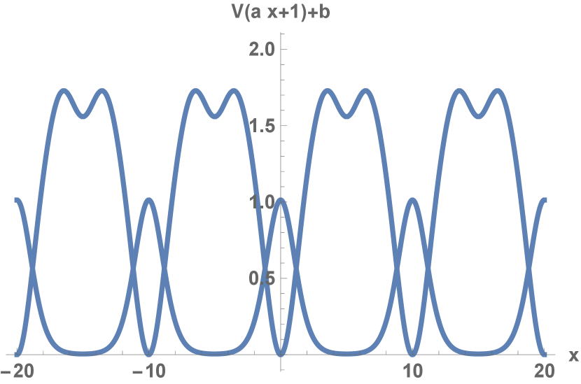
The effective potential for with fermions in the one-loop approximation is given in [6].
| (2.5) |
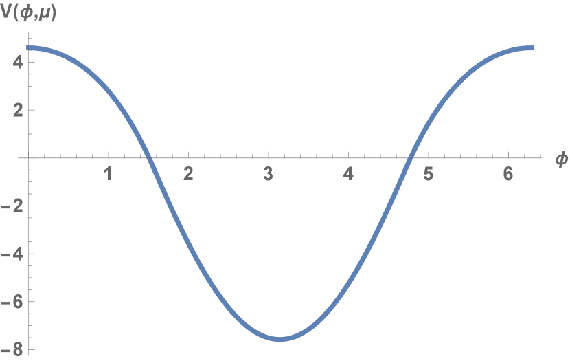
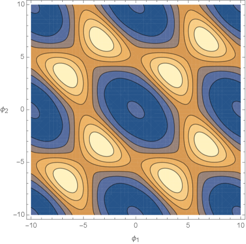
The first term comes from the gauge bosons and the second from the fermions. The potential is shown in figure 1. In this section we wish to calculate the ground state energy for potentials of this type using the Variational Quantum Eigensolver and IBM QISKit. The effective Matrix Model Hamiltonian we consider for is:
| (2.6) |
The first step in quantum simulation is to represent the Hamiltonian in a finite Hilbert space representation which can be mapped to qubits. A convenient basis is the harmonic oscillator basis where the and operators can be represented as:
| (2.7) |
while for the momentum operator we have:
| (2.8) |
The Variational Quantum Eigensolver (VQE) is a hybrid classical-quantum algorithm based on the variational method of quantum mechanic to estimate the ground state energy and ground state wave function of a quantum Hamiltonian. By choosing a variational wave function one minimizes:
| (2.9) |
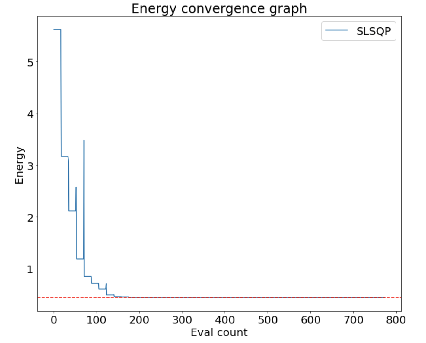
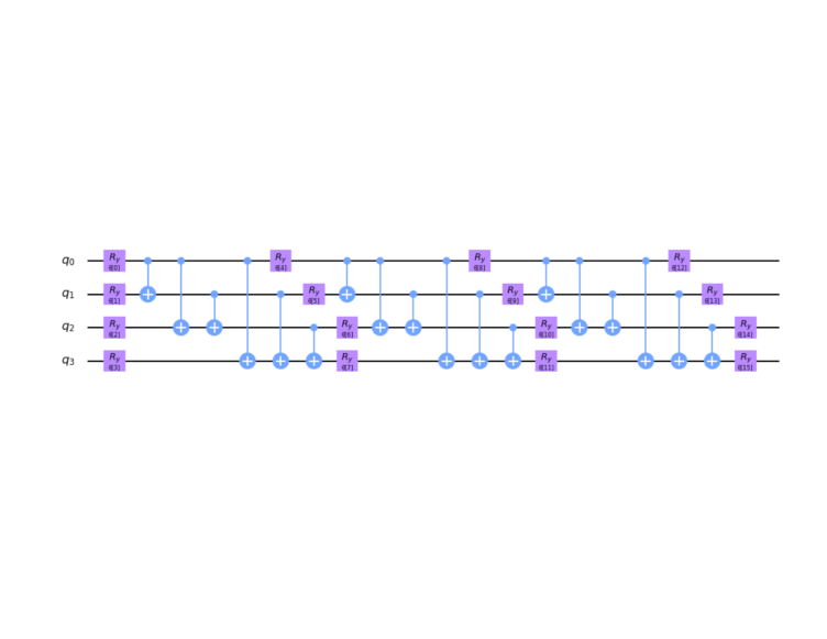
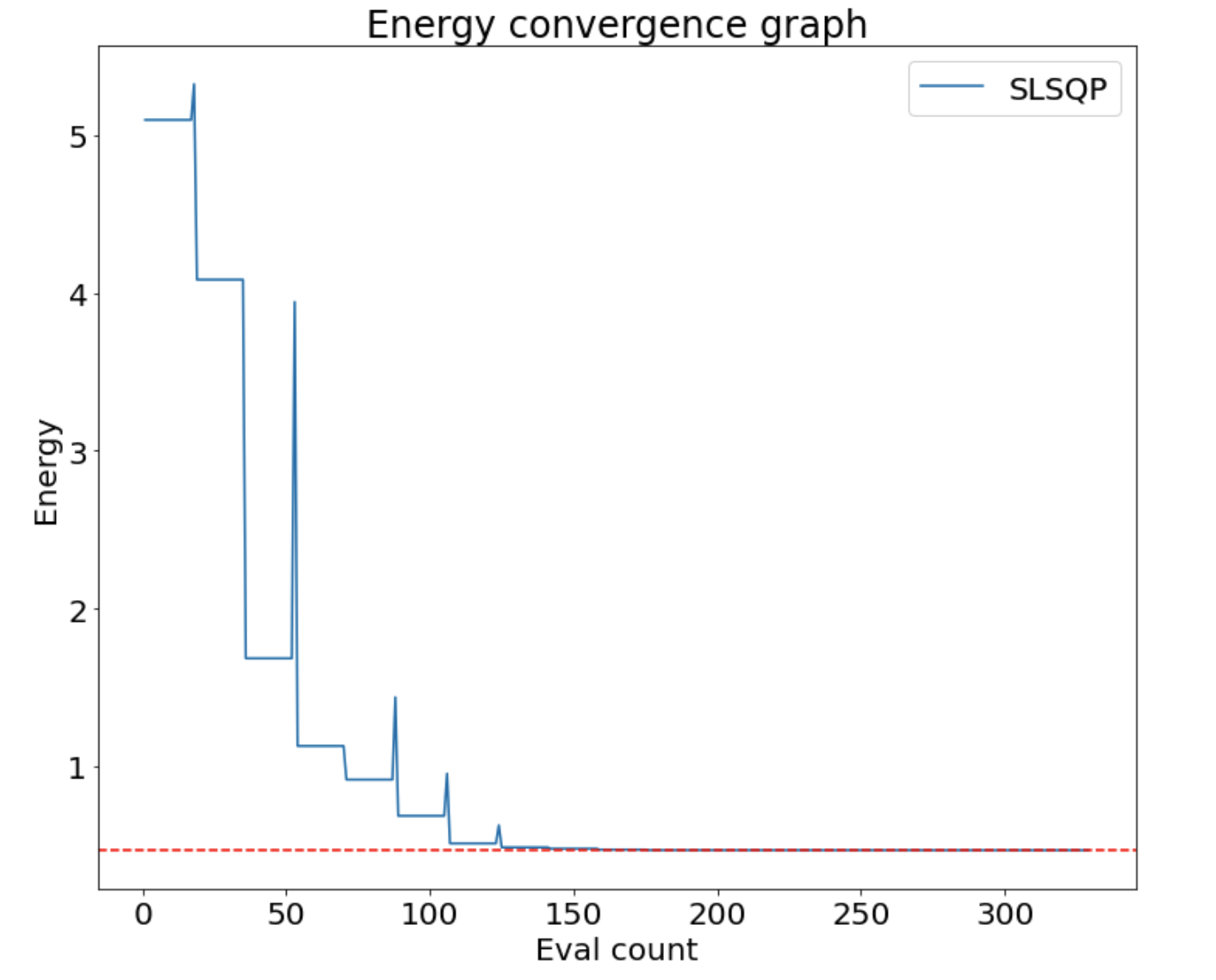
The are angles which parameterize the variational wave function and are represented on the quantum computer in terms of quantum gates. The Hamiltonian is represented in terms of qubits as a expansion of tensor products of two by two matrices given by the Pauli spin matrices plus the two by two identity matrix. One uses an optiimizer to find the minimum of over several iterations and over several runs to determine the least upper bound on the ground state energy. It is this least upper bound which is the result of the VQE that is its estimate to the ground state energy. Using matrices for so the total The Hamiltonian is also a matrix and can be represented by four qubits. Using the VQE and the SLSQP optimizer we find the results in table 1 which are in excellent agreement with classical computation.
| Hamiltonian | Qubits | Paulis | Exact Result | VQE Result |
|---|---|---|---|---|
| with fermion in fundamental | 4 | 71 | 0.4425673 | 0.4426310 |
3 VQE for effective Matrix model for finite temperature
Finite temperature can be included by using the imaginary time formulation with periodic boundary conditions for bosons and antiperiodic boundary conditions for fermions in imaginary time. For finite temperature the effective potential is given by [6]:
| (3.1) |
where:
| (3.2) |
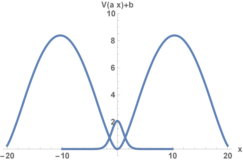
The potential is plotted in figure 4. For small this can be approximated by:
| (3.3) |
For a representative calculation we choose a temperature such that . Then the exact ground state energy is . Using the VQE algorithm we find from table 2, in excellent agreement with the classical computation.
| Hamiltonian | Qubits | Paulis | Exact Result | VQE Result |
|---|---|---|---|---|
| finite temperature | 4 | 55 | .46617183 | 0.46617228 |
4 VQE for effective Matrix Model with finite density
One can derive the one-loop Effective Matrix Model potential for finite density by using the imaginary time formulation and introducing an complex vector potential in the imaginary time direction so the covariant derivative is modified by with . The fermion effective Matrix potential at finite temperature and density can then be expressed as [4]:
For and one has the simplified form:
We plot this potential in figure 6.
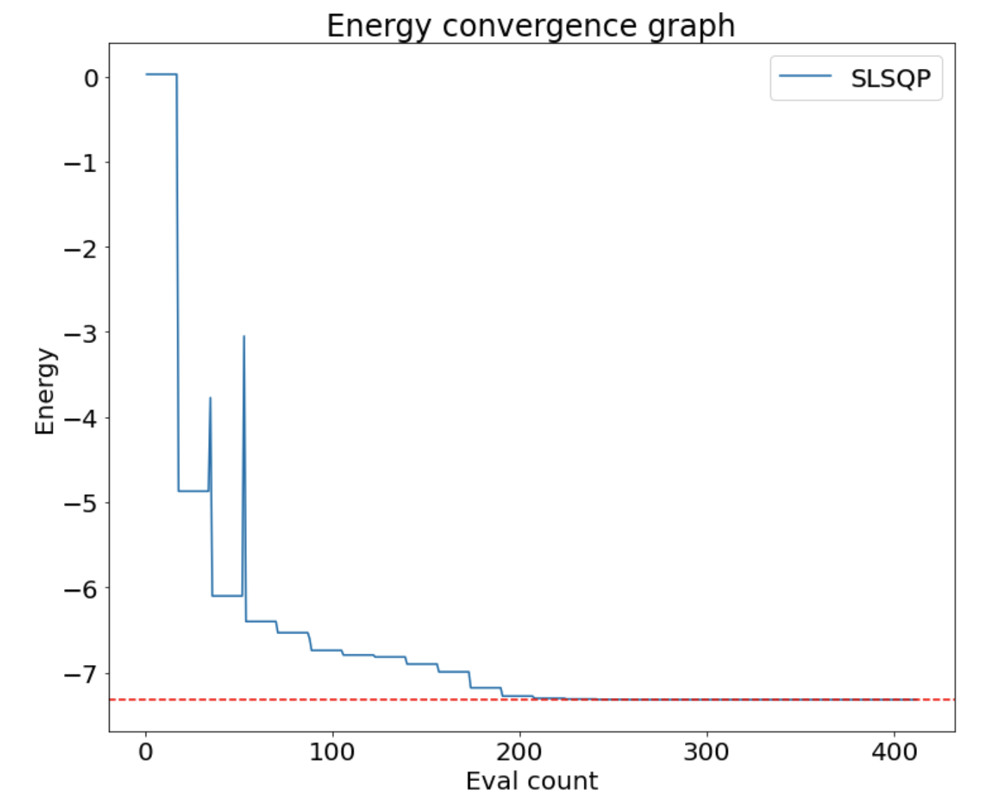
The exact ground state energy . Using the VQE algorithm we find the results from table 3 which are in excellent agreement with the classical computation.
| Hamiltonian | Qubits | Paulis | Exact Result | VQE Result |
|---|---|---|---|---|
| finite density | 4 | 55 | -7.32051788 | -7.32051782 |
5 VQE for effective Matrix model for SU(3)
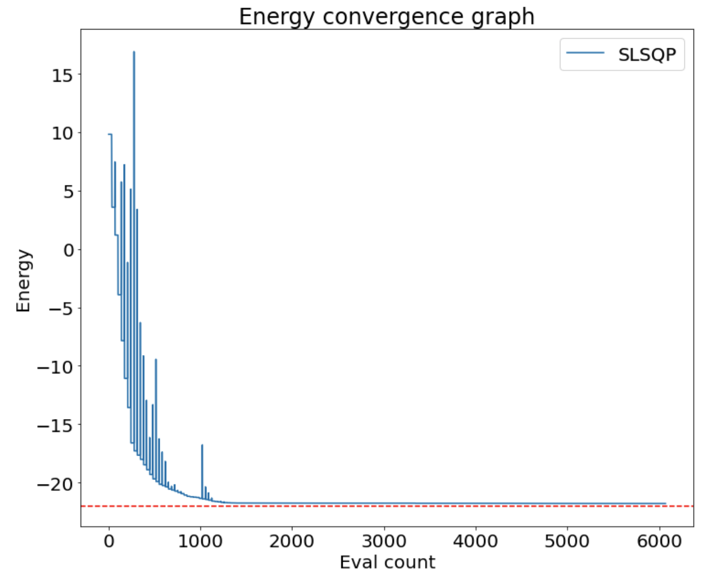
| Hamiltonian | Qubits | Paulis | Exact Result | VQE Result |
|---|---|---|---|---|
| with fermion in fundamental | 8 | 9137 | -21.98808168 | -21.793084965 |
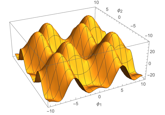
For one can proceed similarly to except is rank two and there are two Wilson lines and . The gauge potential for the Effective Matrix model is parameterized as:
| (5.1) |
and Effective Matrix potential for with one fermion in the fundamental representation is:
| (5.2) |
where:
| (5.3) |
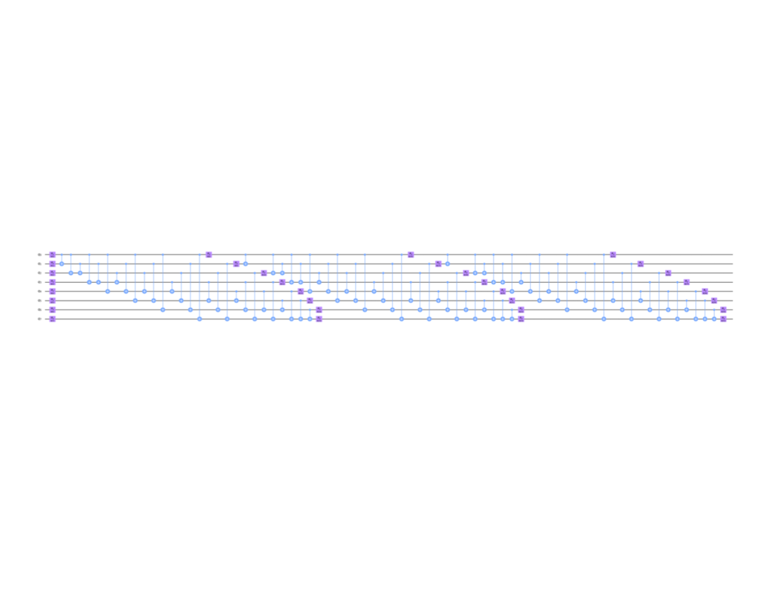
and . Because there are two Wilson line variables we need to use tensor products to construct the Hamiltonian for the VQE. Defining:
| (5.4) |
where and are given by 2.7 amd 2.8. The Hamiltonian is then written as
| (5.5) |
Using matrices for and so the total Hamiltonian is and can be represented by eight qubits. Using the VQE and the SLSQP optimizer we find the results in table 4 which are in excellent agreement with classical computation.
6 Conclusions
In this paper we studied the Effective Matrix Model for gauge theories on a quantum computer. We were able to obtain accurate results for and gauge models including fermion including finite temperature and finite density effects involving nonzero chemical potential using the Variational Quantum Eigensolver (VQE) approach on a IBM quantum computer. It will be interesting to extend computations to include new terms in the Matrix model coming from nonperturbative effects in the equation of state as was done in [2]. Finally by considering inhomogeneous Matrix models which depend on one spatial coordinate, or by studying large rank groups as occur in UV complete theories like string theory or in strongly interacting dark matter models, the effective matrix model may exceed the simulation capabilities of classical computers and thus provide an excellent opportunity for quantum advantage on quantum computers.
Acknowledgements
This material is based upon work supported by the U.S. Department of Energy, Office of Science, National Quantum Information Science Research Centers, Co-design Center for Quantum Advantage (C2QA) under contract number DE-SC0012704. This project was supported in part by the U.S. Department of Energy, Office of Science, Office of Workforce Development for Teachers and Scientists (WDTS). We wish to acknowledge useful discussions on effective Matrix models with Rob Pisarski.
References
- [1] C. Korthals Altes, K. Y. Lee and R. D. Pisarski, “Effective potential for the Wilson line in the standard model,”
- [2] A. Dumitru, Y. Guo, Y. Hidaka, C. P. K. Altes and R. D. Pisarski, “Effective Matrix Model for Deconfinement in Pure Gauge Theories,” Phys. Rev. D 86, 105017 (2012) doi:10.1103/PhysRevD.86.105017 [arXiv:1205.0137 [hep-ph]].
- [3] K. Kashiwa, R. D. Pisarski and V. V. Skokov, “Critical endpoint for deconfinement in matrix and other effective models,” Phys. Rev. D 85, 114029 (2012) doi:10.1103/PhysRevD.85.114029 [arXiv:1205.0545 [hep-ph]].
- [4] K. Shiraishi, “Finite Temperature and Density Effect on Symmetry Breaking by Wilson Loops,” Z. Phys. C 35, 37 (1987) doi:10.1007/BF01561053 [arXiv:1206.6211 [hep-th]].
- [5] K. Shiraishi, “DEGENERATE FERMION AND WILSON LOOP IN (1+1)-DIMENSIONS,” Can. J. Phys. 68, 357-360 (1990) doi:10.1139/p90-056 [arXiv:1801.01647 [hep-th]].
- [6] C. L. Ho and Y. Hosotani, “Symmetry Breaking by Wilson Lines and Finite Temperature Effects,” Nucl. Phys. B 345, 445-460 (1990) doi:10.1016/0550-3213(90)90395-T
- [7] J. L. Davis, “The Moduli space and phase structure of heterotic strings in two dimensions,” Phys. Rev. D 74, 026004 (2006) doi:10.1103/PhysRevD.74.026004 [arXiv:hep-th/0511298 [hep-th]].
- [8] Y. Hosotani, “Dynamical Mass Generation by Compact Extra Dimensions,” Phys. Lett. B 126, 309-313 (1983) doi:10.1016/0370-2693(83)90170-3
- [9] U. Gursoy, S. A. Hartnoll, T. J. Hollowood and S. P. Kumar, “Topology change and new phases in thermal N=4 SYM theory,” JHEP 11, 020 (2007) doi:10.1088/1126-6708/2007/11/020 [arXiv:hep-th/0703100 [hep-th]].
- [10] H. Itoyama and S. Nakajima, “Stability, enhanced gauge symmetry and suppressed cosmological constant in 9D heterotic interpolating models,” Nucl. Phys. B 958, 115111 (2020) doi:10.1016/j.nuclphysb.2020.115111 [arXiv:2003.11217 [hep-th]].
- [11] Y. Hamada, H. Kawai and K. y. Oda, “Eternal Higgs inflation and the cosmological constant problem,” Phys. Rev. D 92, 045009 (2015) doi:10.1103/PhysRevD.92.045009 [arXiv:1501.04455 [hep-ph]].
- [12] P. H. Ginsparg and C. Vafa, “Toroidal Compactification of Nonsupersymmetric Heterotic Strings,” Nucl. Phys. B 289, 414 (1987) doi:10.1016/0550-3213(87)90387-7
- [13] V. P. Nair, A. D. Shapere, A. Strominger and F. Wilczek, “Compactification of the Twisted Heterotic String,” Nucl. Phys. B 287, 402-418 (1987) doi:10.1016/0550-3213(87)90112-X
- [14] A. E. Faraggi and M. Pospelov, “Selfinteracting dark matter from the hidden heterotic string sector,” Astropart. Phys. 16, 451-461 (2002) doi:10.1016/S0927-6505(01)00121-9 [arXiv:hep-ph/0008223 [hep-ph]].
- [15] M. McGuigan, “Dark Horse, Dark Matter: Revisiting the (16)x (16)’ Nonsupersymmetric Model in the LHC and Dark Energy Era,” [arXiv:1907.01944 [hep-th]].
- [16] N. Yamanaka, H. Iida, A. Nakamura and M. Wakayama, “Dark matter scattering cross section and dynamics in dark Yang-Mills theory,” Phys. Lett. B 813, 136056 (2021) doi:10.1016/j.physletb.2020.136056 [arXiv:1910.01440 [hep-ph]].
- [17] T. Duong and M. McGuigan, ”Visualization of higher genus carbon nanomaterials: free energy, persistent current, and entanglement entropy,” 2017 New York Scientific Data Summit (NYSDS), 2017, pp. 1-5, doi: 10.1109/NYSDS.2017.8085055.
- [18] R. Miceli and M. McGuigan, ”Effective matrix model for nuclear physics on a quantum computer,” 2019 New York Scientific Data Summit (NYSDS), 2019, pp. 1-4, doi: 10.1109/NYSDS.2019.8909693.