Effects of 3D Position Fluctuations on Air-to-Ground mmWave UAV Communications
Abstract
Millimeter wave (mmWave)-based unmanned aerial vehicle (UAV) communication is a promising candidate for future communications due to its flexibility and sufficient bandwidth. However, random fluctuations in the position of hovering UAVs will lead to random variations in the blockage and signal-to-noise ratio (SNR) of the UAV-user link, thus affecting the quality of service (QoS) of the system. To assess the impact of UAV position fluctuations on the QoS of air-to-ground mmWave UAV communications, this paper develops a tractable analytical model that jointly captures the features of three-dimensional (3D) position fluctuations of hovering UAVs and blockages of mmWave (including static, dynamic, and self-blockages). With this model, we derive the closed-form expressions for reliable service probability respective to blockage probability of UAV-user links, and coverage probability respective to SNR, respectively. The results indicate that the greater the position fluctuations of UAVs, the lower the reliable service probability and coverage probability. The degradation of these two evaluation metrics confirms that the performance of air-to-ground mmWave UAV systems largely depends on the UAV position fluctuations, and the stronger the fluctuation, the worse the QoS. Finally, Monte Carlo simulations demonstrate the above results and show UAVs’ optimal location to maximize the reliable service and coverage probability, respectively.
Index Terms:
Millimeter wave, unmanned aerial vehicle communications, position fluctuations, blockages, QoS.I Introduction
The advantage of unmanned aerial vehicle (UAV) makes it more likely to be employed as the aerial base station (BS) for future communications, which will significantly satisfy the diversified requirements on data rate, transmission delay, system capacity, etc.[1, 2]. Compared with traditional BSs, UAVs have higher flexibility and lower cost. Therefore, UAV communications have attracted increasing attention and are particularly suitable for on-demand scenarios, such as hot spots or disaster sites where existing communications infrastructures are overloaded or damaged [3]. Meanwhile, to achieve ultra-high data rates, more and more researchers consider millimeter wave (mmWave) with large available bandwidth as the carrier frequency of UAV communications[4]. Such communications are hereinafter called as mmWave UAV communications. mmWave UAV communications have significant advantages in flexibility, system capacity, etc.
One of the critical challenges of deploying mmWave UAVs is that the position and orientation of hovering UAVs, compared to ground BSs, can change randomly due to wind, inaccurate positioning, etc.[5, 6, 7]. Such random variations will lead to random changes in the quality of the UAV-user links, which will lead to unreliable communications. Some innovative studies have investigated the impact of hovering fluctuations of UAVs on mmWave UAV communication systems. For example, the work in [6] experimentally investigated the effect of random fluctuations of hovering UAVs on mmWave signals. It demonstrated that the mismatch of antenna beams caused by the random fluctuations would deteriorate the performance of UAV-to-ground links. The authors in [7, 8] investigated the influence of UAV orientation fluctuations on system outage performance. They showed that the beam misalignment and antenna gain mismatch caused by UAV orientation fluctuations lead to a decline in the reliability of the communication system. The authors in [9] analyzed the effect of UAV attitude angle fluctuations on the antenna orientation, and they proposed a UAV beam training method to improve the accuracy of antenna angle estimation. However, [6, 7, 8, 9] focused on investigating the impact of antenna beam misalignment or poor beam selection caused by hovering UAV fluctuations on system performances.
In addition to the above impacts on antenna beam alignment, fluctuations, especially position fluctuations of UAVs may also significantly impact mmWave blockage characteristics. As we know, mmWave signals are easily blocked by obstacles, and the blockage state is mainly determined by the relative positions of transceivers and obstacles [10]. The random position deviation of hovering UAVs will make the blockage characteristics more randomized, thus affecting the system’s performance. So investigating the influence of UAV position fluctuations on link blockage, then evaluating the QoS is necessary. Specifically, UAV position fluctuation is three-dimensional (3D), and a line-of-sight (LoS) mmWave link may encounter three types of blockages: static blockage caused by static obstacles such as buildings, dynamic blockage caused by moving blockers, and self-blockage caused by the user’s own body[11]. Therefore, it is essential to obtain the relationship between the 3D position fluctuations of hovering UAVs and the three kinds of blockages of mmWave, as well as the impact on the system performance.
The effect of blockages on the mmWave system without considering the position fluctuations of UAVs has been widely studied. For instance, the work in [12, 11, 13, 14, 15, 16] studied the blockage effects of mmWave signals in terrestrial communications. For mmWave UAV communications, the static blockage due to buildings has been studied in [17, 18, 19], and the LoS probability is obtained to guide the deployment of UAVs. In [4, 20, 21], the coverage performance was analyzed under static blockage. Furthermore, the authors in [22] contributed an analytical framework to characterize mmWave backhaul links by considering dynamic blockage, and it is shown that the assistance of UAVs can significantly improve the performance of mmWave backhaul links. The authors in [23] presented a method of optimal deployment, which provided the optimal 3D position and coverage radius of a UAV by considering human blockage. More recently, in [24], the authors experimentally verified the impact of human body on air-to-ground links, and the results showed that the effect depended largely on the hovering UAVs’ positions. However, the above results are obtained under the supposition that the position of the UAV is perfectly stable. This assumption is too ideal because, in practice, the fluctuation of UAVs is unavoidable.
As far as we know, there are few studies on mmWave blockage characteristics under the effect of UAV position fluctuations. In [25], the authors studied the blockage characteristics and beam misalignment considering the hovering fluctuation effect of UAV, and they proposed a UAV deployment and beamforming optimization method to establish robust transmission. However, their theoretical model only analyzed the blockage probability considering UAV position fluctuations. But, more importantly, further system performance analysis still needs improvement. Especially the system reliability analysis under the joint consideration of fluctuations and blockages has yet to be carried out. In addition, in our previous work[26], we developed a theoretical analysis model to study the impact of UAV position fluctuations on UAV-user link blockages and the reliability of air-to-ground mmWave UAV communications. However, the results of [26] are obtained based on a simple model that only considered the height fluctuations of UAVs.
Although the above work provides valuable insights for mmWave UAV communications, more research still needs to be done on the effect of UAV 3D position fluctuations on the system’s QoS. A comprehensive analytical model that builds the relationship between the hovering UAVs’ position fluctuations and the mmWave link’s blockages is greatly requested to benefit from mmWave UAV communications. This is what we are trying to do through this work. The major contributions of this paper are given as follows:
We propose a novel model to analyze the effect of UAV 3D position fluctuations on the QoS of air-to-ground mmWave UAV systems. Different from existing works, this work establishes the theoretical relationship between the position fluctuations of UAVs and the blockages of mmWave links (including static, dynamic, and self-blockages), which enables the evaluation of the blockage characteristics of UAV-user links under position fluctuations. Especially, we find that the dynamic blockage is obviously affected by the random fluctuations of UAV position, and its fluctuation variance is directly proportional to the variance of UAV position fluctuations.
We derive the closed-form expressions for reliable service probability respective to the probability of UAV-user links blockages, and coverage probability respective to the signal-to-noise ratio (SNR), respectively. The results indicate that the greater the position fluctuation strength of the UAV is, the lower the reliable service probability and coverage probability is. Therefore, UAV position fluctuations considerably influence these two QoS metrics of the considered system. To our best knowledge, this is the first work that analytically evaluates the impact of UAV 3D position fluctuations on the QoS of air-to-ground mmWave UAV communication systems while considering the static, dynamic, and self-blockage of mmWave links.
We provide Monte Carlo simulations to verify the theoretical results, and the simulation results also show that there exists an optimal horizontal position and height of UAVs to maximize the reliable service probability and coverage probability, respectively, which help establish reliable air-to-ground mmWave UAV communications.
The rest of this paper is organized as follows: In Section II, we present the system model. In Section III, we analyze the effect of UAV position fluctuation on link blockages. In Section IV, the closed-form expression of reliable service probability is derived, while in Section V, the closed-form expression of coverage probability is derived. Section VI provides the simulation results, and Section VII concludes this paper. Notations used in this paper are given in Table I.
II System Model
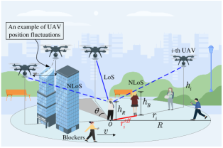
We consider a mmWave UAV communications scenario, as shown in Fig. 1, where ground users are randomly distributed and served by UAVs as aerial BSs. Since obstacles easily block UAV-user links, we assume the user can immediately link to another unblocked link once the current UAV-user link is blocked. Without losing generality, we randomly select a user as the typical user. The typical user’s location is denoted as , where is the height of the typical user. The specific model settings are given as follows:
| Notation | Description |
| Real-time position of the -th UAV under fluctuations. | |
| Mean of the real-time position . | |
| // | Density of UAVs/human blockers/buildings. |
| Velocity of moving human blockers. | |
| 2D distance from the -th UAV to the user. | |
| / | Indicator for dynamic/static blockage for the -th link. |
| Indicator for self-blockage for a single UAV-user link. | |
| Indicator for the -th UAV is available. | |
| / | Number of all/available UAVs. |
II-A UAV Models
This subsection models the position and position fluctuations of UAVs. Since hovering UAVs will fluctuate randomly, the real-time position of each UAV fluctuates randomly around its central position [5, 25]. We denote and as the central position and the real-time position for the -th UAV, respectively. The central positions on the two-dimensional (2D) plane is modeled as a homogeneous Poisson point process (PPP) with density [11]. We assume that the maximum service radius of the UAV is . Therefore, the number of all potential serving UAVs for the typical user is Poisson distributed i.e., . Then, due to the real-time position of the hovering UAV fluctuates randomly, and numerous literature has modeled UAV position fluctuations as Gaussian distributions [27, 7, 5, 28], the exact position of the -th UAV can be modeled as , where is the variance of the UAV position fluctuations. It is clear that the greater the is, the greater the fluctuation is. Therefore, we regard as a measure of UAV position fluctuation strength.
II-B Blockage Models
II-B1 Dynamic Blockage Model
Dynamic blockage due to moving humans has been thoroughly studied in mmWave systems with traditional BSs [12, 11, 13]. Following [11], we assume that humans are located in the region according to a homogeneous PPP of density , and they move randomly at velocity . We define effective blockage length to reflect whether blockage occurs when a human blocker passes through a UAV-user link. The effective blockage length for the -th UAV-user link is , where is the height of the human blocker, . Then, the dynamic blockage of the -th link is modeled as an exponential on-off process with blocking and non-blocking rates of and , respectively [11], where and is simplified to a constant. Moreover, we know that the -th link is dynamically blocked with probability (w.p.) . We define a random variable to indicate whether dynamic blockage occurs on the -th UAV-user link, and can be represented as
| (3) |
where is used for convenience.
II-B2 Static Blockage Model
Static blockage caused by static obstacles (e.g., high-rise buildings) has been well studied in [18, 4, 16] based on random shape theory. We consider the blockage model given in [16] to model the static blockage, and the -th link is blocked with probability , where will be given later. Similar to dynamic blockage, we define to describe whether static blockage occurs on the -th link, and can be represented as
| (6) |
where and , , , and are the density, expected length, and width of the buildings, respectively.
II-B3 Self-Blockage Model
Except for dynamic and static blockages, a fraction of links will also be blocked by the user’s own body. Following [11], we define a sector of angle behind the user as the self-blockage zone. The user himself will block all UAV-user links in this zone. Therefore, the self-blockage probability of a UAV-user link is the probability that the UAV is located in the self-blockage zone. We define an indicative random variable to describe whether self-blockage occurs on a single UAV-user link, and can be represented as
| (9) |
III Effect of Fluctuations on Blockages
This section focuses on obtaining the relationship between UAV position fluctuations and UAV-user link blockages. Specifically, according to (3) and (6), we observe that the probability of dynamic and static blockages of UAV-user link is related to the position of the UAV (i.e., and ). Due to random fluctuations in the UAV’s position, and are randomly changing and only reflect an instantaneous moment’s blockage characteristic. On the one hand, the random variation in the blockage state is detrimental to users, as it will lead to unreliable communications. On the other hand, analyzing the performance of a system at a specific moment is difficult and of limited value. Hence, to evaluate the average performance of the system, it is important to obtain the distribution of and under UAV position fluctuations. Accordingly, in the following, we derive the relevant probability density function (PDF).
III-A Effect of Fluctuations on Dynamic Blockage
Theorem 1.
Proof.
The proof is given in Appendix A. ∎
Remark 1: From Theorem 1, (38) and (39), we can observe that the mean of is independent of the variance of the UAV position fluctuations. However, the variance of is an increasing function of . Therefore, the higher the fluctuation strength of the UAV, the larger the deviation of from its mean .
Then, the relationship between , and average 2D distance is given as follows:
Corollary 1.
and are increasing and decreasing functions of , respectively, . Therefore, the maximum values of can be expressed as
| (11) |
where denotes the maximum value of , . Similarly, we can obtain the maximum value of by replacing in (39) with .
Proof.
The proof is given in Appendix B. ∎
Remark 2: According to Corollary 1, we can conclude that if the UAV is deployed closer to the user, i.e., is smaller, the mean of will be smaller. However, in this case, the variance of will become larger. Therefore, there may be an appropriate to obtain a trade-off between and so that the system can achieve a better QoS.
III-B Effect of Fluctuations on Static Blockage
Corollary 2.
The PDF of can be well approximately modeled as
| (12) |
where and can be seen in the proof, and is a compressed version of .
Proof.
We first derive the PDF of . According to (37), can be approximately modeled as a normal distribution with mean and variance . As a result, we have is normally distributed with mean and variance . Therefore, is log-normally distributed [29], and its PDF is given by . We further denote the cumulative distribution function (CDF) of and as and , respectively. It is easy to get , and by taking the derivative of . Finally, the PDF of is obtained as shown in (12).∎
Using Corollary 2, we can obtain the mean and variance of separately as
| (13) | ||||
| (14) |
Remark 3: From (13) and (14), we can infer that the mean and variance of may also be affected by the position fluctuation of UAV. However, in our system assumption, we can obtain: and , where the detailed proof can be seen in Appendix C. The results indicate that the hardly changes with the position fluctuation of the UAV, which matches the intuition that the dimension of the position fluctuation of the UAV is very small compared to the size of buildings. Therefore, the impact of UAV position fluctuations on the static blockage probability of the link is negligible, and only when the UAV is located at the edge of the building will position fluctuations of the UAV affect the link’ static blockage state.
IV Effect of Fluctuations on Reliable Service
This section analyzes the effect of UAV position fluctuations on the reliable service probability. Since static and self-blockage will lead to permanent blockage, a UAV is available if UAV-user link is not blocked by static blockage and self-blockage. We are more concerned that at least one UAV is available. Due to blockages affecting the system reliability, we propose a new QoS metric in terms of links blockages, called reliable service probability, given by Definition 1.
Definition 1.
A user is said to be in reliable service if at least one UAV is available with a blockage probability not higher than a predefined threshold. The reliable service probability is denoted as and given by
| (15) |
where denotes the probability that UAVs are available, denotes the probability that UAVs are available and the dynamic blockage probability of each link is greater than the threshold . Therefore, the second term of (15) represents the probability that the user is not in a reliable service. Note that will result in , which means there are no UAVs available. So we let . To calculate , we first give the distribution of UAVs availability in the following.
IV-A Distribution of UAVs Availability
We use an indicative random variable to indicate that the -th UAV is available, denotes the probability of , which is also the probability that the -th link is not blocked by static and self-blockage. Then, the distribution of the number of available UAVs is obtained as:
Lemma 1.
The distribution of the number of available UAVs is Poisson distributed with parameter , i.e.,
| (16) |
where .
Proof.
The proof is given in Appendix C. ∎
Then, we derive the closed-form expression of reliable service probability for single and multiple UAV cases according to Definition 1. It indicates that the greater the fluctuation strength of the UAV, the lower the , and the worse the QoS. The specific details are given as follows.
IV-B Reliable Service Probability for Single UAV Case
In this case, we assume that the typical user can only link to one UAV, and denote the UAV as the -th UAV. Let represent the reliable service probability for the single UAV case, it indicates the probability that the -th UAV is available and the dynamic blockage probability of the link is lower than the threshold . Then, can be obtained as shown in Theorem 2.
Theorem 2.
Proof.
Since in this case we only consider one UAV is available, (15) can be rewritten as
| (18) |
where is indeed the probability that the -th UAV is available, i.e., , and . Substituting and into (18), then using Theorem 1, we can get
| (19) |
where the last step is obtained by integrating according to [15, Eq. (3)]. ∎
According to Theorem 2, we can obtain the effect of on the QoS. In (17), and are not affected by according to (47) and (38), respectively. So only is related to , and is an increasing function of , which can be observed from (39), we first analyze the effect of on . Since error function erf is a monotonically function and erf, will show two different effects on . For , erf and decreases as increases. For , erf and increases as increases. However, in the latter situation, the value of is lower, even less than 0.5, which indicates that the QoS is evil, further analyze the effect of on the QoS is almost meaningless. Hence, throughout this paper, we pay more attention to the former case (). We can conclude that the greater the is, the larger the is, the lower the is, and the worse the QoS is. It is worth noting that from the derivation of (IV-B), it can be found that is similar to the CDF of , which is normally distributed according to Theorem 1. Therefore, when changes, the variation of is similar to that of the CDF of . The above analysis is also consistent with this phenomenon. Moreover, for an open area scenario (park/stadium/square)[11], we can rewrite as follows.
Corollary 3.
For an open area communication scenario, can be rewritten as follows:
| (20) |
Proof.
IV-C Reliable Service Probability for Multiple UAVs Case
In this case, we assume that the typical user has more than one UAVs that can be connected, and it will immediately switch to any other available UAV when the currently serving link is blocked. We define as the reliable service probability for this case, it represents the probability that at least one UAV is available with a dynamic blockage probability lower than the predefined threshold . Then, we obtain the approximate as shown in Theorem 3.
Theorem 3.
Proof.
Although Theorem 3 gives an approximate expression of , the expression is not tractable due to . Fortunately, since it is unrealistic to have an infinite number of UAVs in practice, we can assume the maximum number of UAVs is . Then, can be rewritten as:
| (23) |
which is solvable. Furthermore, we can get the lower bound of as shown in Corollary 4.
Corollary 4.
A lower bound of is given by
| (24) |
where and , .
Proof.
According to Theorem 3 and Corollary 4, we can conclude that the larger the is, the smaller the is, and the lower the QoS is, which is consistent with the single UAV case. Similarly, when and , , we can obtain an upper bound of , which is similar to (IV-C) and is omitted for brevity. For an open area scenario, can be obtained by setting , the reason is consistent with the proof of Corollary 3.
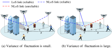
Finally, a graphical example of the impact of on the blockage and the QoS is shown in Fig. 2. This example depicts two snapshots of the links’ blockage status. As we can see, the blockage status and reliable service in the two snapshots is different even though the blockers are the same, which is due to the position fluctuations of the UAV. Moreover, as discussed in Theorem 2 and Corollary 4, the function of reliable service probability has almost similar variation characteristics to the CDF of normal distribution. Therefore, when , the higher the UAV’s fluctuation, the smaller the probability of reliable service. In conclusion, the larger the is, the lower the reliable service probability is, and the worse the QoS is.
V Effect of Fluctuations on Coverage
Section IV evaluated the effect of on reliable service probability, which is defined respective to the blockage probability. This may not capture the full picture of the considered system. Hence, this section refers to coverage probability in terms of SNR as another QoS measurement and evaluates the impact of on this measurement. The coverage probability is defined as follows:
Definition 2.
A user is said to be in coverage if at least one UAV is available with a SNR not smaller than a predefined threshold. The coverage probability is denoted as and given by
| (26) |
where denotes the SNR at the user from the -th UAV, denotes the probability that UAVs are available and the SNR of each link is smaller than the threshold . Therefore, the second term of (26) denotes the probability that the user is not in coverage, and we consider that when since in this case there are no available UAVs.
Next, we first develop a channel model for the considered system. Then, the SNR at the user is expressed, and the coverage probability for single and multiple UAV cases are derived.
V-A Channel Model
Since UAV-user link is only dynamically blocked when the UAV is available, the LoS probability of the -th link can be expressed as follows:
| (27) |
and we assume that the channel between UAVs and the target user is based on the dominant LoS. Therefore, the channel gain of the -th UAV-user link is given by [30]:
| (28) |
where is the path loss (PL) at unit distance, is parameter of the PL, is the 3D distance from the -th UAV to the typical user. Then, the SNR at the user is given by
| (29) |
where is the transmit power of the UAV and is the noise power. It is clear that is a function of random variables and , which means that the position fluctuations of UAVs will affect the . Therefore, the coverage probability given in Definition 2 can capture these effects.
V-B Coverage Probability for Single UAV Case
Similar to , we define as the coverage probability for the single UAV case, it represents the probability that the -th UAV is available and the SNR of the -th link is not smaller than the threshold . Therefore, using Definition 2 and similar to (18) and (IV-B), we first can get
| (30) |
Then, is approximately obtained as shown in Theorem 4.
Theorem 4.
Proof.
The proof is given in Appendix D. ∎
Since Marcum Q-function is a standard function that is easy to compute[7], using Theorem 4, we can quickly evaluate the QoS of the considered system without resorting to time-consuming simulation, especially the impact of UAV position fluctuations on the coverage probability. In addition, when an open area communication scenario is considered, the coverage probability can be obtained by setting , the reason is consistent with the proof of Corollary 3.
V-C Coverage Probability for Multiple UAVs Case
Similar to , we define as the coverage probability for the multiple UAVs case, it represents the probability that at least one UAV is available with a SNR not smaller than the threshold . Then, we can obtain as follows:
Theorem 5.
The coverage probability for the multiple UAVs case is given by
| (32) |
where , .
Proof.
Similar to (23), given the limited number of UAVs in practice, can be rewritten as
| (34) |
Furthermore, a lower bound of is obtained as shown in Corollary 5.
Corollary 5.
A lower bound of is given by
| (35) |
where and , .
VI Simulation Results
This section performs extensive simulations to confirm the theoretical results. For the simulation, we consider that the blockers are uniformly distributed within a circular area centered at the typical user with a radius of m. The movement of the human blockers is generated by a random way-point mobility model[31], where human blockers will randomly select a direction and walk in that direction at the speed of 1 ms, the time of moving in that direction is uniformly distributed for [0, 60] seconds. The detailed simulation parameters are given in Table II.
| Parameters | Values |
| Height of the user/blockers, / | 1.4/1.8 m [11] |
| Density of moving blockers, | 0.01, 0.02 blm2 |
| Density of static buildings, | 100 sblkm2[11] |
| Non-blocking rate, | bls [11] |
| Fluctuation strength of UAVs, | 0 to 0.2 m[28] |
| Transmit power of UAV, | dBm |
| Noise power, | dBm [32] |
| SNR threshold, | dB[22] |
| Size of static buildings, | m m[16] |
| Path loss parameters, , | 2, [32] |
VI-A Analysis of Reliable Service Probability
VI-A1 Single UAV case
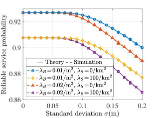
Fig. 3 visualizes the impact of on . First, as expected, the higher the is, the lower the is. Therefore, we can get the higher the degree of UAV position fluctuations, the worse the system reliability. Then, under the same , the higher the density of blockers is, the smaller the is. This is reasonable because the fewer blockers on the UAV-user link, the smaller the blockage probability and the higher the reliability of the link. Therefore, the QoS in the scenario with static buildings is worse than in the open scenario without. However, in the low region (), even for different , the value of is the same and hardly changes with . This happens because under our simulation parameter settings, in a low region, and is independent of and . The details are described as: Using (39), we can get is close to 0 when is small. For example, when , and other parameters given in Table II, , so the fluctuation of is extremely small and is closely around its mean value . Therefore, the probability that is less than the threshold is close to 1 since , i.e., , and the value of mainly depends on .
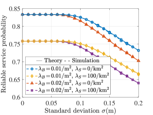
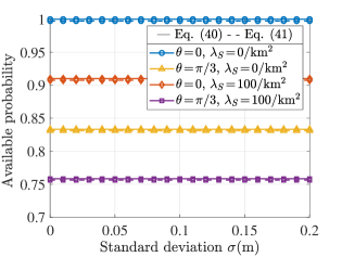
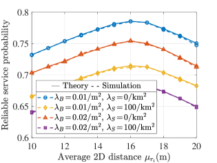
Fig. 4 depicts the curves of given in (C) and (47), respectively. First, it is clear that the impact of on is negligible. Then, the curves with are actually the (when ) in Fig. 3. Therefore, at a low region, and has little impact on it.
Fig. 5 shows how the average 2D distance from the UAV to the typical user impacts . As we can see, there exists an optimal (about 16 m in our simulation scenario) for maximizing . According to Corollary 1 and Theorem 2, on the one hand, we know that the greater the is, the smaller the is, so the larger the is. On the other hand, however, is an increasing function of , and the greater the is, the smaller the is. Therefore, these two factors lead to the existence of an optimum for maximizing .
VI-A2 Multiple UAVs case
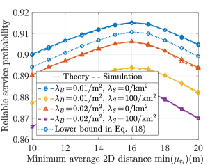
Fig. 6 and Fig. 7 plot reliable service probability according to (23), where . As we can see, the larger the is, the smaller the is. Therefore, the influence of UAV position fluctuations on the QoS of this case is the same as that of the single UAV case. However, comparing these two cases, it is obvious that . This mainly benefits from the multi-connectivity strategy, i.e., when the current link is blocked, the user can quickly switch to other available UAVs to reduce the blockage. Therefore, using multiple UAVs can alleviate the impact of blockage on the QoS. Then, similar to the single UAV case, when is small (), we can infer , so , and . This indicates that in the considered scenario, is independent of and at a low region. Noted that in this case, we assume that all UAVs are distributed on a ring with an inner diameter of an outer diameter of m. Fig. 7 studies the impact of on , it is clear that an optimal exists for maximizing . The reason is a combination of two factors, as described in the analysis of Fig. 5. In addition, Fig. 7 compares and a lower bound of in (24) for and . It can be observed that the value of is slightly greater than the lower bound.
VI-B Analysis of Coverage Probability
VI-B1 Single UAV case
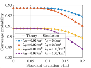
Fig. 8 studies the effect of on the coverage probability for the single UAV case. First, we observe that decreases as increases. This happens because strong fluctuations in the UAV position will result in strong fluctuations in the SNR , which increases the probability that will fall below the given threshold . Therefore, decreases with the increase of . Then, it is clear that in the low region (), even for different , the value of is the same and hardly changes with . This happens because in a low region, the effect of on the is negligible. Therefore, the probability that is less than is close to 0, as is slightly greater than in our simulation settings, i.e., . Therefore, and is independent of and by using (V-B) and (47).
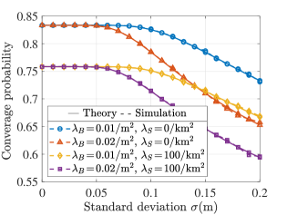
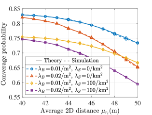
Fig. 9 investigates the impact of average 2D distance from the UAV to the user on . It is clear that the larger the is, the smaller the is. The reason is that increasing will increase the distance between transceivers and the blockage probability. Therefore, the SNR received by the user is reduced, and is decreased according to (V-B). The result is also consistent with Theorem 4. Specifically, is an increasing function of , and increase with the increase of according to the characteristics of Marcum Q-function. Therefore, is a decreasing function of . Additionally, combined with the analysis of reliable service probability in Fig. 5, one thing we found very interesting is that when is at a relatively low region, the user has a higher probability of getting reliable service and coverage. After all, selecting an appropriate can improve the service quality.
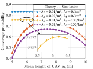
Fig. 10 shows as a function of average UAV height . As we expected, there is an optimal that maximizes . Two factors cause the result: On the one hand, when the UAV is at a low height, the LoS probability will be small. The resulting small channel gain increases the probability of SNR falling below the given threshold, thereby reducing coverage. On the other hand, for the UAV with high height, even though the link is in LoS, the increasing distance between the user and the UAV will also reduce the SNR of the link, thus leading to a low probability of coverage. Therefore, these two contributors eventually lead to the existence of an optimum for maximum .
VI-B2 Multiple UAVs case
Fig. 11 plots the effect of on coverage probability . Similar to the single UAV case in Fig. 8, we can see that in a low region (), the for different is the same and hardly changes with . However, when is larger, the decreases with the increase of . Meanwhile, when comparing Fig. 11 and Fig. 8, it is obvious that , the reason is that using multiple UAVs can reduce the blockage of the link, thus improving the SNR and the coverage performance. Note that in this case, we assume that all UAVs are distributed on a ring with an inner diameter of an outer diameter of m.
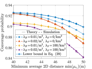
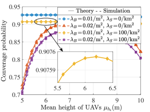
Fig. 12 shows the impact of on . It is clear that the decrease with the increase of , the reason is similar to the analysis of Fig. 9 of the single UAV case, and is also consistent with the general conclusion that the service quality of edge users is generally the worst. In addition, Fig. 12 compares the and a low bound of in (35) for and . We observe that the value of in (34) is slightly greater than the lower bound of , which is reasonable. Finally, Fig. 13 proves that there is an optimal for maximum . The reason is a combination of two factors, as described in the analysis of Fig. 10.
VII Conclusion
In this paper, we studied the critical issues affecting the QoS of air-to-ground mmWave UAV communication systems, especially those arising from the random position fluctuations of hovering UAVs. Accordingly, we considered the reliable service probability respective to links blockages, and the coverage probability respective to SNR as the system’s key QoS measures. Then, we derived the closed-form expressions to evaluate the impact of UAV position fluctuations on these two QoS metrics. Our results indicated that the larger the position fluctuations of the UAV, the smaller the reliable service probability, and the smaller the coverage probability. Therefore, unlike ground mmWave communications, the QoS of the air-to-ground mmWave UAV communication system largely depends on the position fluctuations of the UAV. Specifically, the fluctuation will cause random changes in the blockage characteristic and the SNR of the link, thus resulting in unreliable communications. Fortunately, we theoretically analyzed the effect of UAV position fluctuations on link blockages and SNR, and the relevant results made it possible to quickly evaluate the QoS of the system under different levels of UAV position fluctuations. In addition, according to the simulation results, we find the optimal horizontal position and height of the UAV to maximize the reliable service probability and the coverage probability, respectively, which helps establish reliable mmWave UAV communications.
Appendix A Proof of Theorem 1
We denote the PDF of as , and according to (3), can first be expressed by taking the derivative of the corresponding CDF , i.e., . Therefore, it is important to analyze the CDF of in order to obtain . Since and are Gaussian distributed, follows a Rician distribution [28], and the PDF can be denoted as , where , denotes the modified Bessel function of the first kind of zero order. In general, the 2D distance from the UAV to the user is far greater than the fluctuation strength of the UAV, i.e., . Therefore, can be well approximated by a Gaussian random variable according to [33, 34], and then, the PDF of can be rewritten as follows:
| (37) |
Then, we can get and . Finally, using the conclusions in [35, 36], can be well modeled as a Gaussian distribution with mean and variance . Among them, and are given as follows:
| (38) | ||||
| (39) |
Therefore, can finally be obtained as shown in (10).
Appendix B Proof of Corollary 1
First, we take the derivative of (38) with respect to and have
| (40) |
The reason why (40) is greater than 0 is that in the considered communication system, generally, the height of the UAV is higher than that of the user, i.e., . Therefore, is an increasing function of . Next, to obtain the relationship between and , we denote the first and second terms of in (39) as and respectively. Then, we can get
| (41) |
which indicates that decreases with the increase of . Similarly, we have
| (42) |
which means that is a decreasing function of . Then, also is a decreasing function of . Therefore, we can conclude that is a decreasing function of . The reason why (42) is less than 0 is as follows: In our system, is the speed of the moving humans, and are the height of the moving humans and user, respectively. Generally speaking, these parameters are fixed values in the considered communications scenario, and by using Table II. As such, is only a fraction of , and even for as high as bl/m2[11], the value of is only 0.025. Therefore, . However, is usually several times or even more than ten times of and . All in all, .
Appendix C Proof of Lemma 1
We assume that the blockage of each link is independent. Therefore, given the total number of UAVs , the distribution of the number of available UAVs can be expressed as [11]:
| (43) |
Since is Poisson distributed, can be obtained as [11, Lemma 2], where is given in Subsection II-A. Therefore, we can finally get
| (44) |
where the available probability is calculated as follows: Using (6) and (9), the conditional probability that the -th UAV is available is , and it is obviously that . Therefore, to obtain the marginal probability , we first need to take the average of over the distribution of , and according to (37), follows a Gaussian distribution with mean value . However, is still a random variable since the center positions of the UAVs are modeled as a PPP. As a result, we can get
| (45) |
the PDF of is [11]. Therefore, we can get
| (46) |
For further insight, we further approximate as follows: We know that , and due to . Therefore, according to the characteristics of error function. Then, since the size of the buildings are , the maximum value of density of the buildings is , and the maximum value of is given by , where the inequality is obtained based on the fact that the value of and are larger than 1 in practice, and the result indicates that , i.e., . We have , and in practice. Hence, , and the value of mainly depends on , i.e., , which verifies our insights in Remark 3. Therefore we can assume that , and then,
| (47) |
Fig. 4 further illustrates the accuracy of this approximation.
Appendix D Proof of Theorem 4
According to (V-B), we can get , where is given in (47). Hence, we only need to calculate . With the aid of (27), (28) and (29), we can get
| (48) |
which is related to the CDF of . Therefore, to obtain , it is necessary to calculate the CDF mentioned above by considering random variables , , and . To this end, we define an indicator random variable as follows:
| (49) |
and analyze the CDF of . First, we have and . Therefore, is Rician distributed, and the PDF is , where . Then, using (27) and (3), we have , and follows a normal distribution as shown in Theorem 1. Therefore, also follows a normal distribution with mean and variance where and are given in (38) and (39), respectively. Next, we will prove that the randomness of mainly depends on . In this case, the task of calculating the CDF of can be converted to calculating the CDF of . We first prove that the random variable can be approximated by its mean . Using the proof of Corollary 1, we know that , , and is several orders of magnitude smaller than that of for our system setup. Therefore, we first can get since in practice. Then, we have . Moreover, we can get with the aid of Table II. Therefore, due to is usually several times or even more than ten times of and . In addition, we have [32]. Based on the above discussion, we can conclude that , i.e., . Therefore, has little impact on . As a result, we can assume that , and then, substituting (38) into (49), can be rewritten as
| (50) |
and the objective of calculating the CDF of can be simplified as calculating the CDF of . Let us denote the CDF of as . Since is Rician distributed, can be expressed in terms of the Marcum Q-function as follows [37, 38]:
| (51) |
where is the Marcum Q-function and is defined as
| (52) |
Finally, with the aid of (V-B), (48), (49), (50) and (51), we have
| (53) |
References
- [1] B. P. Sahoo, D. Puthal, and P. K. Sharma, “Toward Advanced UAV Communications: Properties, Research Challenges, and Future Potential,” IEEE Internet of Things Magazine, vol. 5, no. 1, pp. 154–159, 2022.
- [2] L. Bai, Z. Huang, and X. Cheng, “A Non-Stationary Model With Time-Space Consistency for 6G Massive MIMO mmWave UAV Channels,” IEEE Transactions on Wireless Communications, vol. 22, no. 3, pp. 2048–2064, 2023.
- [3] C. Ge, R. Zhang, D. Zhai, Y. Jiang, and B. Li, “UAV-Correlated MIMO Channels: 3-D Geometrical-Based Polarized Model and Capacity Analysis,” IEEE Internet of Things Journal, vol. 10, no. 2, pp. 1446–1460, 2023.
- [4] W. Yi, Y. Liu, Y. Deng, and A. Nallanathan, “Clustered UAV Networks With Millimeter Wave Communications: A Stochastic Geometry View,” IEEE Transactions on Communications, vol. 68, no. 7, pp. 4342–4357, 2020.
- [5] M. Najafi, H. Ajam, V. Jamali, P. D. Diamantoulakis, G. K. Karagiannidis, and R. Schober, “Statistical Modeling of the FSO Fronthaul Channel for UAV-Based Communications,” IEEE Transactions on Communications, vol. 68, no. 6, pp. 3720–3736, 2020.
- [6] S. G. Sanchez, S. Mohanti, D. Jaisinghani, and K. R. Chowdhury, “Millimeter-Wave Base Stations in the Sky: An Experimental Study of UAV-to-Ground Communications,” IEEE Transactions on Mobile Computing, vol. 21, no. 2, pp. 644–662, 2022.
- [7] M. T. Dabiri, M. Rezaee, V. Yazdanian, B. Maham, W. Saad, and C. S. Hong, “3D Channel Characterization and Performance Analysis of UAV-Assisted Millimeter Wave Links,” IEEE Transactions on Wireless Communications, vol. 20, no. 1, pp. 110–125, 2021.
- [8] M. T. Dabiri, H. Safi, S. Parsaeefard, and W. Saad, “Analytical Channel Models for Millimeter Wave UAV Networks Under Hovering Fluctuations,” IEEE Transactions on Wireless Communications, vol. 19, no. 4, pp. 2868–2883, 2020.
- [9] W. Wang and W. Zhang, “Jittering effects analysis and beam training design for UAV millimeter wave communications,” IEEE Transactions on Wireless Communications, vol. 21, no. 5, pp. 3131–3146, 2021.
- [10] J. Zhao, J. Liu, J. Jiang, and F. Gao, “Efficient Deployment With Geometric Analysis for mmWave UAV Communications,” IEEE Wireless Communications Letters, vol. 9, no. 7, pp. 1115–1119, 2020.
- [11] I. K. Jain, R. Kumar, and S. S. Panwar, “The Impact of Mobile Blockers on Millimeter Wave Cellular Systems,” IEEE Journal on Selected Areas in Communications, vol. 37, no. 4, pp. 854–868, 2019.
- [12] M. F. Özkoç, A. Koutsaftis, R. Kumar, P. Liu, and S. S. Panwar, “The Impact of Multi-Connectivity and Handover Constraints on Millimeter Wave and Terahertz Cellular Networks,” IEEE Journal on Selected Areas in Communications, vol. 39, no. 6, pp. 1833–1853, 2021.
- [13] I. K. Jain, R. Kumar, and S. Panwar, “Driven by Capacity or Blockage? A Millimeter Wave Blockage Analysis,” in 2018 30th International Teletraffic Congress (ITC 30), 2018.
- [14] M. Gapeyenko, A. Samuylov, M. Gerasimenko, D. Moltchanov, S. Singh, M. R. Akdeniz, E. Aryafar, N. Himayat, S. Andreev, and Y. Koucheryavy, “On the Temporal Effects of Mobile Blockers in Urban Millimeter-Wave Cellular Scenarios,” IEEE Transactions on Vehicular Technology, vol. 66, no. 11, pp. 10 124–10 138, 2017.
- [15] M. Gapeyenko, A. Samuylov, M. Gerasimenko, D. Moltchanov, S. Singh, E. Aryafar, S. P. Yeh, and S. Andreev, “Analysis of Human-Body Blockage in Urban Millimeter-Wave Cellular Communications,” in 2016 IEEE International Conference on Communications (ICC), 2016.
- [16] T. Bai, R. Vaze, and R. W. Heath, “Analysis of Blockage Effects on Urban Cellular Networks,” IEEE Transactions on Wireless Communications, vol. 13, no. 9, pp. 5070–5083, 2014.
- [17] F. Li, C. He, X. Li, J. Peng, and K. Yang, “Geometric Analysis-Based 3D Anti-Block UAV Deployment for mmWave Communications,” IEEE Communications Letters, vol. 26, no. 11, pp. 2799–2803, 2022.
- [18] M. Gapeyenko, D. Moltchanov, S. Andreev, and R. W. Heath, “Line-of-Sight Probability for mmWave-Based UAV Communications in 3D Urban Grid Deployments,” IEEE Transactions on Wireless Communications, vol. 20, no. 10, pp. 6566–6579, 2021.
- [19] A. Al-Hourani, S. Kandeepan, and S. Lardner, “Optimal LAP Altitude for Maximum Coverage,” IEEE Wireless Communications Letters, vol. 3, no. 6, pp. 569–572, 2014.
- [20] X. Guo, C. Zhang, F. Yu, and H. Chen, “Coverage Analysis for UAV-Assisted MmWave Cellular Networks Using Poisson Hole Process,” IEEE Transactions on Vehicular Technology, vol. 71, no. 3, pp. 3171–3186, 2022.
- [21] X. Shi and N. Deng, “Modeling and Analysis of mmWave UAV Swarm Networks: A Stochastic Geometry Approach,” IEEE Transactions on Wireless Communications, 2022.
- [22] M. Gapeyenko, V. Petrov, D. Moltchanov, S. Andreev, N. Himayat, and Y. Koucheryavy, “Flexible and Reliable UAV-Assisted Backhaul Operation in 5G mmWave Cellular Networks,” IEEE Journal on Selected Areas in Communications, vol. 36, no. 11, pp. 2486–2496, 2018.
- [23] M. Gapeyenko, I. Bor-Yaliniz, S. Andreev, and H. Yanikomeroglu, “Effects of Blockage in Deploying mmWave Drone Base Stations for 5G Networks and Beyond,” in 2018 IEEE International Conference on Communications Workshops (ICC Workshops), 2018, pp. 1–6.
- [24] M. Badi, S. Gupta, D. Rajan, and J. Camp, “Characterization of the Human Body Impact on UAV-to-Ground Channels at Ultra-Low Altitudes,” IEEE Transactions on Vehicular Technology, vol. 71, no. 1, pp. 339–353, 2022.
- [25] S. G. Sanchez and K. R. Chowdhury, “Robust 60GHz Beamforming for UAVs: Experimental Analysis of Hovering, Blockage and Beam Selection,” IEEE Internet of Things Journal, pp. 1–1, 2020.
- [26] C. Ma, X. Li, X. Xie, X. Ma, C. He, and Z. J. Wang, “Effects of Vertical Fluctuations on Air-to-Ground mmWave UAV Communications,” IEEE Wireless Communications Letters, pp. 1–1, 2022.
- [27] J.-Y. Wang, Y. Ma, R.-R. Lu, J.-B. Wang, M. Lin, and J. Cheng, “Hovering UAV-Based FSO Communications: Channel Modelling, Performance Analysis, and Parameter Optimization,” IEEE Journal on Selected Areas in Communications, vol. 39, no. 10, pp. 2946–2959, 2021.
- [28] M. T. Dabiri, S. M. S. Sadough, and M. A. Khalighi, “Channel Modeling and Parameter Optimization for Hovering UAV-Based Free-Space Optical Links,” IEEE Journal on Selected Areas in Communications, vol. 36, no. 9, pp. 2104–2113, 2018.
- [29] R. Ulrich and J. Miller, “Information Processing Models Generating Lognormally Distributed Reaction Times,” Journal of Mathematical Psychology, vol. 37, no. 4, pp. 513–525, 1993.
- [30] Y. Zeng, Q. Wu, and R. Zhang, “Accessing From the Sky: A Tutorial on UAV Communications for 5G and Beyond,” Proceedings of the IEEE, vol. 107, no. 12, pp. 2327–2375, 2019.
- [31] A. Merwaday and smail Güven, “Handover Count Based Velocity Estimation and Mobility State Detection in Dense HetNets,” IEEE Transactions on Wireless Communications, vol. 15, no. 7, pp. 4673–4688, 2016.
- [32] C. Zhang, L. Zhang, L. Zhu, T. Zhang, Z. Xiao, and X.-G. Xia, “3D Deployment of Multiple UAV-Mounted Base Stations for UAV Communications,” IEEE Transactions on Communications, vol. 69, no. 4, pp. 2473–2488, 2021.
- [33] J. Sijbers, A. J. den Dekker, P. Scheunders, and D. Van Dyck, “Maximum-likelihood estimation of Rician distribution parameters,” IEEE Transactions on Medical Imaging, vol. 17, no. 3, pp. 357–361, 1998.
- [34] S. Pajevic and P. J. Basser, “Parametric and non-parametric statistical analysis of DT-MRI data,” Journal of magnetic resonance, vol. 161, no. 1, pp. 1–14, 2003.
- [35] E. Díaz-Francés and F. J. Rubio, “On the existence of a normal approximation to the distribution of the ratio of two independent normal random variables,” Statistical Papers, vol. 54, no. 2, pp. 309–323, 2013.
- [36] D. V. Hinkley, “On the ratio of two correlated normal random variables,” Biometrika, vol. 56, no. 3, pp. 635–639, 1969.
- [37] P. Y. Kam and R. Li, “A new geometric view of the first-order Marcum Q-function and some simple tight erfc-bounds,” in 2006 IEEE 63rd Vehicular Technology Conference, vol. 5. IEEE, 2006, pp. 2553–2557.
- [38] H.-C. Yang and M.-S. Alouini, “Closed-form formulas for the outage probability of wireless communication systems with a minimum signal power constraint,” IEEE Transactions on Vehicular Technology, vol. 51, no. 6, pp. 1689–1698, 2002.