Effects of correlated magnetic noises from shared control lines on two-qubit gate

Fault-tolerant quantum computation requires synergy over a large number of physical qubits: Depending on the error rate, a logical qubit based on the surface code can take thousands of physical qubits to encode.(Fowler et al., 2012; Preskill, 2018) This motivates the construction of large scale quantum computational devices. Despite that single-qubit and two-qubit gates with the gate fidelity above the fault-tolerant threshold had been achieved across various platforms,(Ballance et al., 2016; Noiri et al., 2022; Xue et al., 2022) upto now only 72 qubits were realized experimentally based on the superconducting circuit,(Google Quantum, 2023) and it was not until recently that the logical qubit could be demonstrated.(Zhao et al., 2022; Krinner et al., 2022)

One of the difficulties involved in building a desired large scale device capable of implementing error correction code is to maintain uniformity in the characteristic parameters across all the underlying qubits. (Laucht et al., 2021; Meyer et al., 2023) In this regard, semi-conductor based spin qubits stands out with a unique advantage of being compatible with the matured industrial fabrication technologies. (Veldhorst et al., 2017) Following this approach, several proposals for building scalable devices had been put-forward.(Hill Charles et al., 2015; Veldhorst et al., 2017; Li et al., 2018; Gonzalez-Zalba et al., 2021) Later in experiments, a two-dimensional crossbar array containing $36\times 36$ gates were reported,(Bavdaz et al., 2022) while recently a two-dimensional array of 16 qubits with the inter-dot coupling above 10GHz was experimentally realized in terms of the SiGe based hole-spin quantum dots. (Borsoi et al., 2023)

Unlike the traditional few-qubit setups for the proof-of-principle demonstrations where each qubit could be individually addressable, those scalable proposals usually features common control lines that borrowed from the CMOS or crossbar architectures.(Veldhorst et al., 2017; Li et al., 2018) On one hand they reduce the complexity of control layers and enable the integration of plenty of qubits, on the other hand, however, the noises imposed on such shared control lines may affect several qubits at the same time, thus result in correlated errors among the qubits. Although cryo-CMOS techniques have been developed for the purpose of qubit operation,(Patra et al., 2018; Charbon et al., 2021) since those noises differ from the influences of the local environment that experienced by individual qubit, it would be still useful to distinguish between those noises in order to further reduce the control errors that associated with the multi-qubit operations.

In this work, we explore several possible sources of correlated magnetic noises in a simplified two-qubit model motivated by the crossbar proposal for scalable quantum computation. (Li et al., 2018) To distinguish among those noises, we apply a method based on the interleaved randomized benchmarking (IRB). (Magesan et al., 2012a) In additional to the standard random circuit in the IRB, we introduce an additional measurement induced decoherence process to selective address certain components of the noisy quantum channel. Although the investigation is based on a specific model, the method should be generally applicable also to other scenarios.

This paper is organized as follows: In Sec. II, we introduce the model and derive the magnetic field at the qubit location. In Sec. III, different possible magnetic noises are discussed, with the corresponding perturbative Hamiltonian given explicitly. In Sec. IV, the method based on the IRB is introduced and applied to distinguish between two particular correlated magnetic noises. Further discussions are provided in Sec. V, and we draw the conclusion in Sec. VI. Technique details can be found in the Appendices.

Following several papers about the proposal of crossbar architecture for salable quantum computation, (Hill Charles et al., 2015; Veldhorst et al., 2017; Li et al., 2018) here we consider the following simplified model that schematically shown in FIG. 1(a). The system features an array of equally spacing parallel wires carrying currents in alternating directions. For an estimation of the magnetic field generated by the $n$-th wire at the qubit position, we use an effective media description such that (Jackson, 1999)

where $\mu_{\mathrm{eff}}$ is the effective

permeability of the media, $I$ is the current through the $n$-th wire with the current direction indicated by the unit vector $\mathbf{e}_{n}$. $\mathbf{r}_{n}$ is the position vector in the $x$-$z$ plane jointing from the wire to the spin qubit. The total magnetic field experienced by the qubit then amounts to the sum over the individual contributions from each wire

Specifically, for a qubit located at $(x,0,0)$ under the configuration of FIG. 1(a), the total magnetic field is given by

and

Here, $B_{0}=\mu_{\mathrm{eff}}I/(2\pi z_{0})$ is the magnetic field generated by a single wire provided that the qubit is located right below the wire with the distance $z_{0}$. $r_{n,j}=\sqrt{x_{n,j}^{2}+z_{0}^{2}}$ and $x_{n,j}$ with $j=1,2$ are defined respectively as follows:

The magnetic field profile calculated according to Eq. (3) is shown in FIG. 1(b). In particular, the magnetic field in the $z$ direction is insensitive to the qubit position near the center between adjacent wires, i.e., odd multiples of $L$. Therefore, the frequency of the qubit that operated at such locations will be insensitive to the qubit’s displacements along $x$ to the first order. (Li et al., 2018) The exact sum in Eq. (3) can be carried out, giving the magnetic field at those ideal operation points $x_{k}\equiv(2k+1)L$ as follows

where the dimensionless quantity $\zeta=\pi z_{0}/(2L)$. Similarly, one can also obtain the magnetic field at $x=2kL$ as

which provides the $B_{x}$ noise insensitive operation points for the qubit.

If the qubit is located away from $x_{k}$, provided that $z_{0}\ll L$ and $|x-x_{k}|\ll L$ then simplification for the magnetic field at the qubit location can be still made. This is achieved by restricting the sum over $n$ in Eq. (3) to the nearest two wires [cf. the orange dashed box in FIG. 1(a)]. To ensure the agreement between the overall magnitude for $B$ at the ideal operation point $x=x_{k}$, one could introduce a calibration coefficient which we take as $\lambda_{k}=B(x_{k})/[b_{k,1}(x_{k})+b_{k,2}(x_{k})]$, such that

Here, $\mathbf{b}_{n,j}$ is obtained from Eq. (1) by replacing $\mathbf{r}_{n}$ and $\mathbf{e}_{n}$ with $\mathbf{r}_{n,j}$ and $\mathbf{e}_{n,j}\equiv(-1)^{j-1}\mathbf{e}_{y}$, respectively. In FIG. 1(b), we also show the magnetic field for $k=0$ calculated from this approximation.

In order to implement two-qubit gates in a crossbar architecture, spins are usually shuttled close to each other such that their mutual exchange interaction can induce entanglement among the spin qubits. (Li et al., 2018) In this sense, current fluctuations in a shared control wire, or a shift of the qubits positions due to mutual charge interaction, acts as a source of noise in the two-qubit operation but in a correlated way. Our goals in this section is to provide a description of such correlated noise at the Hamiltonian level.

The standard model for two-spin

qubits operating in the $(1,1)$ charge configuration is well know, (Burkard, 1999; Meunier et al., 2011) which can be described by the following Hamiltonian upto an overall constant

where $J$ is the exchange interaction which depends on the tunneling coupling as well as the detuning between the two spin qubits, $\omega=\omega_{1}+\omega_{2}$ and $\delta\omega=\omega_{1}-\omega_{2}+\delta\omega_{\mathrm{cor}}$ are the sum as well as the difference of local Zeeman splittings $\omega_{1}$ and $\omega_{2}$ at the two qubits locations, while $\delta\omega_{\mathrm{cor}}$ is a correction due to the mixture of different charge states. (Fang, 2023)

The local Zeeman splittings $\omega_{1}$ and $\omega_{2}$ could be affected in a correlated way, e.g., when the noisy source acts on the both qubits. To be more specific, let us consider the configurations shown in FIG. 2 where the two spin qubits are shuttled next to each other in a row along the $x$-axis, typical for implementing controlled phase operation or spin-to-charge conversion. (Li et al., 2018) As analyzed in the previous section, we shall focus on the magnetic fields generated only by the nearest wires [cf. FIG. 1(b)]. Thus the Zeeman splittings for the two qubits in the absence of noises are

Here, $g$ is the g-factor for the spin qubit, $\mu_{\mathrm{B}}$ is the Bohr magneton, and the angle $\theta=\arctan z_{0}/L$. In general, the perturbation Hamiltonian through the mechanisms shown in FIG. 2 could be written into the following form,

while the specific values $\delta\omega_{x}$ and $\delta\omega_{z}$ depend on the details of the noisy scenarios. For the case of FIG. 2(a) with a perturbation $\delta I$ on the central wire, they are given by

and $\delta B_{0}=\mu_{\mathrm{eff}}\delta I/(2\pi z_{0})$. Instead, for the position shifts scheme as shown in FIG. 2(b), the values are

For comparison, if the current fluctuations $\delta I_{1}$ and $\delta I_{2}$ on the two side wires colored in black in FIG. 2(a) act independently from each other, the resulting perturbation Hamiltonian would be

where

for $i=1,2$ and $\alpha=x,z$, while $\delta B_{i}=\mu_{\mathrm{eff}}\delta I_{i}/(2\pi z_{0})$. Because here the noise is not due to a correlated source, thus the perturbation Eq. (16) is formally different from Eq. (12), expect for special situations, e.g. $\delta I_{1}=\delta I_{2}$ or $\delta I_{1}=-\delta I_{2}$, where the perturbation Eq. (16) coincide with the form of the correlated perturbation.

In the presence of noises, the actual implementation of a quantum gate deviates from the ideal one and this usually degrades the gate fidelity. However, in the context of highly integrated device implementation with shared controls where the noisy source could affects several qubits at the same time, it would be more useful to reveal the structure, e.g., the correlation, of the underlying noises instead of knowing the gate fidelity alone.

In this section, we investigate the correlated noisy effects of the model configuration in FIG. 2(a) by the interleaved randomized benchmarking (IRB). (Magesan et al., 2012a) Our scheme is illustrated in FIG. 3, where

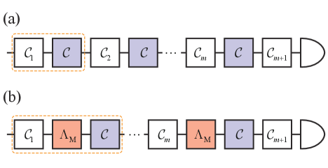
in additional to the standard circuit implementing the IRB. We introduced a measurement process $\Lambda_{\mathrm{M}}$ in between the random Clifford gates and the gate of interest $\hat{U}_{\mathrm{c}}$. By chosen the basis for the measurement process, certain components of the noisy channel could be selected, such that one can distinguish between the two particular cases $\delta I_{1}=\delta I_{2}$ and $\delta I_{1}=-\delta I_{2}$ based on the scenario of FIG. 2(a), here we refer them as the correlated and the anti-correlated noisy perturbations.

For simplicity, we shall assume that in the ideal case $\hat{U}_{\mathrm{c}}$ is also an element from the two-qubit Clifford group $\mathcal{C}_{2}$. This can be achieved from time evolution of the Hamiltonian $\hat{H}$ with the following conditions: (Fang, 2023)

where $k$ is any positive integer. With the above conditions, in the computational basis one has

which belongs to $\mathcal{C}_{2}$ up to an overall phase factor.

The actually implemented gate of interest (denoted as $\hat{U}$) evolves from the full Hamiltonian $\hat{H}+\delta\hat{H}$ and, in the presence of magnetic noises, it

deviates from $\hat{U}_{\mathrm{c}}$. The associated effect of the gate error on time evolution can be formally written in terms of a quantum channel $\Lambda_{\mathrm{c}}$ given by

where $\delta\hat{U}=\hat{U}_{\mathrm{c}}^{\dagger}\hat{U}$. Thus the time evolution of the actual gate is written as $\hat{U}\hat{\rho}\hat{U}^{\dagger}=\mathcal{C}\circ\Lambda_{\mathrm{c}}[\hat{\rho}]$ with $\mathcal{C}[\hat{\rho}]=\hat{U}_{\mathrm{c}}\hat{\rho}\hat{U}_{\mathrm{c}}^{\dagger}$.

Following the standard approach (see also Appendix A for a brief review), (Magesan et al., 2012b, a) we prepared the two-qubit system in the initial state $|\uparrow,\uparrow\rangle$ and performed the usual randomized benchmarking (RB) to extract the depolarization parameter $p$ associated with noise channel $\Lambda$ for the random Clifford gates. For simplicity, we assume a gate independent noise channel $\Lambda$ such that the zero-th order fitting model is applicable to extract $p$. Then by interleaving the actual implementation of $\hat{U}_{\mathrm{c}}$ in between each random Clifford gate [cf. FIG. 3(a)], one obtains a modified depolarization parameter $p_{\mathrm{c}}$ that associates with the combined noisy channel $\Lambda_{\mathrm{c}}\circ\Lambda$. From $p_{\mathrm{c}}$ and $p$ the average error rate of $\Lambda_{\mathrm{c}}$ could be estimated from (Magesan et al., 2012a)

where $d$ is the dimension of the Hilbert space. In the absence of noises for implementing the random Clifford gates, $p=1$ and Eq. (21) reduces to the well known RB result $(d-1)(1-p_{\mathrm{c}})/d$.(Magesan et al., 2011, 2012b)

From the above approach, the average error rate for the actual implementation of the gate $\hat{U}_{\mathrm{c}}$ is simulated and shown in FIG. 4(a). The result suggests that $r_{C}^{\mathrm{est}}$ obtained from the standard IRB is symmetric with respective to rotations in the $\delta I_{1}$-$\delta I_{2}$ plane, i.e., $r_{C}^{\mathrm{est}}$ depends only on $\sqrt{\delta I_{1}^{2}+\delta I_{2}^{2}}$. This is more clearly seen by comparing the two special cases with $\delta I_{1}=\delta I_{2}$ and $\delta I_{1}=-\delta I_{2}$ as shown in the lower panel of FIG. 4(a), where the calculated $r_{C}^{\mathrm{est}}$ overlaps with each other, even though those two cases represent completely different correlations among the perturbations applied to the side wires [cf. FIG. 2(a)].

To better distinguish between the correlated and the anti-correlated cases, we modify the gate sequence in the standard IRB protocol, which is illustrated in FIG. 3(b). As mentioned before, the main difference here is to introduce a measurement induced decoherence process, given in term of a noisy channel $\Lambda_{\mathrm{M}}[\hat{\rho}]=\hat{P}\hat{\rho}\hat{P}^{\dagger}+\hat{Q}\hat{\rho}\hat{Q}^{\dagger}$, where $\hat{P}$ and $\hat{Q}$ are complementary projection operators satisfying $\hat{P}+\hat{Q}=\hat{I}$. Introducing $\Lambda_{\mathrm{M}}$ is motivated by the fact that the insensitive of the standard IRB circuit to $\delta I_{1}$ and $\delta I_{2}$ could be related to the symmetry of the perturbation Hamiltonian. In particular, one can show that for the perturbation term $\delta\hat{H}$ given by Eq. (16), there are two dark states for each of the two special cases, i.e., $\delta\hat{H}_{\lambda}|D_{i}\rangle_{\lambda}=0$ with $\lambda\in\{\mathrm{S},\mathrm{A}\}$, where $\delta\hat{H}_{\lambda}$ is defined as follows

The specific form of those dark states are listed in the Appendix B. Furthermore, the projectors $\hat{P}_{\lambda,i}=|D_{i}\rangle_{\lambda}\langle D_{i}|$ satisfy $\hat{P}_{\mathrm{S},i}\hat{P}_{\mathrm{A},j}=0$. Therefore, projection with $\hat{P}_{\mathrm{S},i}$ ($\hat{P}_{\mathrm{A},i}$) during the implementation of the random circuit will reduce the effects of noisy perturbation in the anti-correlated (correlated) case and lead to higher sequence fidelity, thus enables the distinguishing between the two situations.

Based on the scheme of FIG. 3(b), the sequence fidelity from a particular realization of the random circuit becomes

where $\mathcal{C}_{m+1}=[\prod_{i=1}^{m}\mathcal{C}\circ\mathcal{C}_{i}]^{-1}$. Then by averaging $F_{\mathrm{seq}}$ over $N_{\mathrm{avg}}$ realizations over the random circuits, one has

where $\tilde{p}_{\mathrm{c}}$ is the depolarization parameter associated with the combined depolarization noisy channels $[\Lambda_{\mathrm{c}}\circ\Lambda_{\mathrm{M}}\circ\Lambda]_{\mathrm{d}}$, after taking the twirling operation over the two-qubit Clifford group. (Dankert et al., 2009; Magesan et al., 2012b) Alternatively, removing $\mathcal{C}\circ\Lambda_{\mathrm{c}}$ from Eq. (23) provides a circuit that gives rise to a referential value for the sequence fidelity, whose average leads to the depolarization parameter $\tilde{p}$ associated with $[\Lambda_{\mathrm{M}}\circ\Lambda]_{\mathrm{d}}$. Thus by inserting $\tilde{p}$ and $\tilde{p}_{\mathrm{c}}$ into Eq. (21), one can extract another error rate $\tilde{r}_{C}^{\mathrm{est}}$ associated with gate of interest.

With properly chosen basis for the measurement related projection operator $\hat{P}$, the error rate $\tilde{r}_{C}^{\mathrm{est}}$ could distinguish between the correlated and anti-correlated noises cases. This is shown in FIG. 4(b) for $\hat{P}=|\mathrm{T}_{0}(1,1)\rangle\langle\mathrm{T}_{0}(1,1)|$, where $|\mathrm{T}_{0}(1,1)\rangle$ is the triplet state $|\uparrow,\downarrow\rangle+|\downarrow,\uparrow\rangle$ and also one of the dark states for $\delta\hat{H}_{\mathrm{A}}$. Here, the error rate shows asymmetry as $\delta I_{1}$ and $\delta I_{2}$ varying, and the error rate grows more slowly for the correlated noise perturbation as $\delta I_{1}$ and $\delta I_{2}$ increasing.

Although here we only analysis through a particular perturbation $\delta\hat{H}$ that described by the configuration of FIG. 2(a), the idea of introducing measurement induced decoherence to distinguish noisy correlations should be also applicable to other types of noisy sources, for example, apart from alternating current-carrying wires, other way of generating the magnetic field gradient include the use of micromagnets,(Tokura et al., 2006; Pioro-Ladriere et al., 2008) as well as the Overhauser fields from polarized nuclear spins.(Baugh et al., 2007, 2008) However, in order to construct $\tilde{r}_{C}^{\mathrm{est}}$ that will be sensitive to the noisy correlation, the proper choice of projection operators $\hat{P}$ and $\hat{Q}$ are crucial. To find out those operators, one may wish to enable simpler calculation instead of the full IRB simulations. In fact, we found similar asymmetry behavior in the depolarization parameter $\tilde{p}_{\mathrm{c}}$ of $[\Lambda_{\mathrm{c}}\circ\Lambda_{\mathrm{M}}\circ\Lambda]_{\mathrm{d}}$. Notice that this is directly related to the twirling of $\Lambda_{\mathrm{c}}\circ\Lambda_{\mathrm{M}}\circ\Lambda$ under the two-qubit Clifford group. Thus for theoretical analysis, it is useful to first consider $[\Lambda_{\mathrm{c}}\circ\Lambda_{\mathrm{M}}\circ\Lambda]_{\mathrm{d}}$ instead of $\tilde{r}_{C}^{\mathrm{est}}$.

The sequence fidelity depends also on the system initial state, thus choosing proper initial state could be also useful to distinguish the noisy correlations. For example, suppose the initial state of the two-qubit system is $|\mathrm{T}_{0}(1,1)\rangle\propto|\uparrow,\downarrow\rangle+|\downarrow,\uparrow\rangle$, since this state is also a dark state of $\delta\hat{H}_{\mathrm{A}}$ [cf. Eq. (34)], thus calculating with this initial state amounts to applying the projection operator $\hat{P}$ at the beginning and end of the random circuit. Throughout the calculation we have assumed that the two-qubit system is prepared in the $|\uparrow,\uparrow\rangle$ state. For spin qubits based on the double quantum dot, this state can be prepared by adiabatically changing the detuning through the $\mathrm{S}$-$\mathrm{T}_{+}$ anti-crossing that induced with the transverse field of micromagnet. (Wu et al., 2014; Chesi et al., 2014)

For the purpose of illustration, we did not apply realistic parameters in the simulation. In silicon based double quantum dot, the exchange coupling above $10\mathrm{MHz}$ had been measured,(Veldhorst et al., 2015) while for the crossbar system, the magnetic field was designed such that $\delta\omega\sim 10\mathrm{MHz}$ and $\omega\sim 100\mathrm{MHz}$. (Li et al., 2018) Also, the calculations were performed in the absence of qubit relaxation or dephasing, and the dynamical aspect of the current fluctuation in $\delta I_{1}$ and $\delta I_{2}$ are ignored. The detailed treatment of those effects are out of the current scope and will be addressed in the future works.

In this paper, we have explored correlated magnetic noise in a two-qubit model stimulated by the recent proposals of scalable quantum computation in semi-conductor based spin qubits. With the method introduced here, we could distinguish between the correlated and anti-correlated noisy cases from their different magnetic field dependence of the error rate, obtained from the interleaved randomized bechmarking protocol by using the modified random circuit. The key idea is to introduce a measurement based docherence process such that certain component of the noisy channel associated with the correlated noise could be singled out.

References

- Fowler et al. (2012) A. Fowler, M. Mariantoni, J. M. Martinis, and A. N. Cleland, Phys. Rev. A 86 (2012).
- Preskill (2018) J. Preskill, Quantum 2, 79 (2018).
- Ballance et al. (2016) C. J. Ballance, T. P. Harty, N. M. Linke, M. A. Sepiol, and D. M. Lucas, Phys. Rev. Lett. 117, 060504 (2016).
- Noiri et al. (2022) A. Noiri, K. Takeda, T. Nakajima, T. Kobayashi, A. Sammak, G. Scappucci, and S. Tarucha, Nature 601, 338 (2022).
- Xue et al. (2022) X. Xue, M. Russ, N. Samkharadze, B. Undseth, A. Sammak, G. Scappucci, and L. M. K. Vandersypen, Nature 601, 343 (2022).
- Google Quantum (2023) A. I. Google Quantum, Nature 614, 676 (2023).
- Zhao et al. (2022) Y. Zhao, Y. Ye, H.-L. Huang, Y. Zhang, D. Wu, H. Guan, Q. Zhu, Z. Wei, T. He, S. Cao, F. Chen, T.-H. Chung, H. Deng, D. Fan, M. Gong, C. Guo, S. Guo, L. Han, N. Li, S. Li, Y. Li, F. Liang, J. Lin, H. Qian, H. Rong, H. Su, L. Sun, S. Wang, Y. Wu, Y. Xu, C. Ying, J. Yu, C. Zha, K. Zhang, Y.-H. Huo, C.-Y. Lu, C.-Z. Peng, X. Zhu, and J.-W. Pan, Phys. Rev. Lett. 129, 030501 (2022).
- Krinner et al. (2022) S. Krinner, N. Lacroix, A. Remm, A. Di Paolo, E. Genois, C. Leroux, C. Hellings, S. Lazar, F. Swiadek, J. Herrmann, G. J. Norris, C. K. Andersen, M. Muller, A. Blais, C. Eichler, and A. Wallraff, Nature 605, 669 (2022).
- Laucht et al. (2021) A. Laucht, F. Hohls, N. Ubbelohde, M. F. Gonzalez-Zalba, D. J. Reilly, S. Stobbe, T. Schroder, P. Scarlino, J. V. Koski, A. Dzurak, C.-H. Yang, J. Yoneda, F. Kuemmeth, H. Bluhm, J. Pla, C. Hill, J. Salfi, A. Oiwa, J. T. Muhonen, E. Verhagen, M. D. LaHaye, H. H. Kim, A. W. Tsen, D. Culcer, A. Geresdi, J. A. Mol, V. Mohan, P. K. Jain, and J. Baugh, Nanotechnology 32, 162003 (2021).
- Meyer et al. (2023) M. Meyer, C. Deprez, T. R. van Abswoude, I. N. Meijer, D. Liu, C.-A. Wang, S. Karwal, S. Oosterhout, F. Borsoi, A. Sammak, N. W. Hendrickx, G. Scappucci, and M. Veldhorst, Nano Lett. 23, 2522 (2023).
- Veldhorst et al. (2017) M. Veldhorst, H. G. J. Eenink, C. H. Yang, and A. S. Dzurak, Nat. Commun. 8, 1766 (2017).
- Hill Charles et al. (2015) D. Hill Charles, P. Eldad, J. Hile Samuel, G. House Matthew, F. Martin, R. Sven, Y. Simmons Michelle, and L. Hollenberg Lloyd C., Sci. Adv. 1, e1500707 (2015).
- Li et al. (2018) R. Li, L. Petit, D. P. Franke, J. P. Dehollain, J. Helsen, M. Steudtner, N. K. Thomas, Z. R. Yoscovits, K. J. Singh, S. Wehner, L. M. K. Vandersypen, J. S. Clarke, and M. Veldhorst, Sci. Adv. 4, eaar3960 (2018).
- Gonzalez-Zalba et al. (2021) M. F. Gonzalez-Zalba, S. de Franceschi, E. Charbon, T. Meunier, M. Vinet, and A. S. Dzurak, Nat. Electron. 4, 872 (2021).
- Bavdaz et al. (2022) P. L. Bavdaz, H. G. J. Eenink, J. van Staveren, M. Lodari, C. G. Almudever, J. S. Clarke, F. Sebasatiano, M. Veldhorst, and G. Scappucci, npj Quantum Inf. 8 (2022).
- Borsoi et al. (2023) F. Borsoi, N. W. Hendrickx, V. John, M. Meyer, S. Motz, F. van Riggelen, A. Sammak, S. L. de Snoo, G. Scappucci, and M. Veldhorst, Nat. Nanotechnol. (2023), 10.1038/s41565-023-01491-3.
- Patra et al. (2018) B. Patra, R. M. Incandela, J. P. G. van Dijk, H. A. R. Homulle, L. Song, M. Shahmohammadi, R. B. Staszewski, A. Vladimirescu, M. Babaie, F. Sebastiano, and E. Charbon, IEEE J. Solid-State Circuits 53, 309 (2018).
- Charbon et al. (2021) E. Charbon, M. Babaie, A. Vladimirescu, and F. Sebastiano, IEEE Microwave Mag. 22, 60 (2021).
- Magesan et al. (2012a) E. Magesan, J. M. Gambetta, B. R. Johnson, C. A. Ryan, J. M. Chow, S. T. Merkel, M. P. da Silva, G. A. Keefe, M. B. Rothwell, T. A. Ohki, M. B. Ketchen, and M. Steffen, Phys. Rev. Lett. 109, 080505 (2012a).
- Jackson (1999) J. D. Jackson, Classical Electrodyanmics (John Wiley & Sons, Inc., United States, 1999).
- Burkard (1999) G. Burkard, Phys. Rev. B 60, 11404 (1999).
- Meunier et al. (2011) T. Meunier, V. E. Calado, and L. M. K. Vandersypen, Phys. Rev. B 83, 121403 (2011).
- Fang (2023) Y. Fang, arXiv: 2312.12892v1 (2023).
- Magesan et al. (2012b) E. Magesan, J. M. Gambetta, and J. Emerson, Phys. Rev. A 85, 042311 (2012b).
- Magesan et al. (2011) E. Magesan, J. M. Gambetta, and J. Emerson, Phys. Rev. Lett. 106, 180504 (2011).
- Dankert et al. (2009) C. Dankert, R. Cleve, J. Emerson, and E. Livine, Phys. Rev. A 80, 012304 (2009).
- Tokura et al. (2006) Y. Tokura, W. G. van der Wiel, T. Obata, and S. Tarucha, Phys. Rev. Lett. 96, 047202 (2006).
- Pioro-Ladriere et al. (2008) M. Pioro-Ladriere, T. Obata, Y. Tokura, Y.-S. Shin, T. Kubo, K. Yoshida, T. Taniyama, and S. Tarucha, Nat. Phys. 4, 776 (2008).
- Baugh et al. (2007) J. Baugh, Y. Kitamura, K. Ono, and S. Tarucha, Phys. Rev. Lett. 99, 096804 (2007).
- Baugh et al. (2008) J. Baugh, Y. Kitamura, K. Ono, and S. Tarucha, Phys. Status Solidi C 5, 302 (2008).
- Wu et al. (2014) X. Wu, D. R. Ward, J. R. Prance, D. Kim, J. K. Gamble, R. T. Mohr, Z. Shi, D. E. Savage, M. G. Lagally, M. Friesen, S. N. Coppersmith, and M. A. Eriksson, Proc. Natl. Acad. Sci. 111, 11938 (2014).
- Chesi et al. (2014) S. Chesi, Y.-D. Wang, J. Yoneda, T. Otsuka, S. Tarucha, and D. Loss, Phys. Rev. B 90, 235311 (2014).
- Veldhorst et al. (2015) M. Veldhorst, C. H. Yang, J. C. C. Hwang, W. Huang, J. P. Dehollain, J. T. Muhonen, S. Simmons, A. Laucht, F. E. Hudson, K. M. Itoh, A. Morello, and A. S. Dzurak, Nature 526, 410 (2015).
- Emerson et al. (2005) J. Emerson, R. Alicki, and K. Zyczkowski, J. Phys. B At. Mol. Opt. 7, s347 (2005).