Effects of head modeling errors on the spatial frequency representation of MEG

It is common practice in MEG and EEG modeling to express the total current as a superposition of two components, i.e.,

$$\mathbf{J}\left(\mathbf{r}^{\prime}\right)=\mathbf{J}^{P}\left(\mathbf{r}^{\prime}\right)+\mathbf{J}^{v}\left(\mathbf{r}^{\prime}\right),$$

(1)

where $\mathbf{J}^{P}\left(\mathbf{r}^{\prime}\right)$ represents the physiologically interesting primary current and $\mathbf{J}^{v}\left(\mathbf{r}^{\prime}\right)$ is the associated passive volume current component that completes the loop of electric current in the brain tissue. On the basis of the Coulomb force, the passive volume current is of the form

$$\mathbf{J}^{v}\left(\mathbf{r}^{\prime}\right)=\sigma\mathbf{E}=-\sigma\nabla V,$$

(2)

where $\sigma$, $\mathbf{E}$, and $V$ are the electric conductivity, the electric field, and the electric potential, respectively. The second equality in equation (2) is valid when the time derivative of the magnetic field $\mathbf{B}$ is insignificant, which is the case in MEG and EEG [16]. If we assume a piecewise homogeneous conductor head model with $N_{S}$ conductivity boundary surfaces, the magnetic field due to $\mathbf{J}\left(\mathbf{r}^{\prime}\right)$ is given by Geselowitz’ formula [11, 16]

$$\mathbf{B}\left(\mathbf{r}\right)=\mathbf{B}_{0}\left(\mathbf{r}\right)+\frac{\mu_{0}}{4\pi}\sum_{l=1}^{N_{S}}\left(\sigma_{l}^{-}-\sigma_{l}^{+}\right)\int_{S_{l}^{\prime}}V\left(\mathbf{r}^{\prime}\right)\frac{\mathbf{r}-\mathbf{r}^{\prime}}{\absolutevalue{\mathbf{r}-\mathbf{r}^{\prime}}^{3}}\times d\mathbf{S}^{\prime}_{l},$$

(3)

where

$$\mathbf{B}_{0}\left(\mathbf{r}\right)=\frac{\mu_{0}}{4\pi}\int_{v^{\prime}}\mathbf{J}^{P}\left(\mathbf{r}^{\prime}\right)\times\frac{\mathbf{r}-\mathbf{r}^{\prime}}{\absolutevalue{\mathbf{r}-\mathbf{r}^{\prime}}^{3}}\ dv^{\prime}$$

(4)

is the contribution by primary currents, $v^{\prime}$ is the total head volume, and $\sigma_{l}^{-}$ and $\sigma_{l}^{+}$ denote conductivities of the inner and outer regions relative to $S_{l}$. The second term on the right hand side of (3) is the contribution by volume currents, which we will denote as $\mathbf{B}_{vol}$. We need the electric potential $V$ in order to calculate $\mathbf{B}_{vol}$ and hence the total magnetic field. Below we review the expressions to obtain discrete values of $V$ on the boundaries that we may thus use to approximate and discretize $\mathbf{B}$.

Here, we give an overview of the CC BEM approach. The LC requires only a slight modification, as will be pointed out. More comprehensive reviews may be found in [6, 8, 31, 33, 35].

The electric potential $V(\mathbf{r})$ for a field point $\mathbf{r}$ on the $k$^th surface $S_{k}$ is given intrinsically by [16, 31]

$$V\left(\mathbf{r}\right)=V_{\infty}\left(\mathbf{r}\right)-\frac{1}{2\pi}\sum_{l=1}^{N_{S}}\frac{\sigma_{l}^{-}-\sigma_{l}^{+}}{\sigma_{k}^{-}+\sigma_{k}^{+}}\int_{S_{l}^{\prime}}V\left(\mathbf{r}^{\prime}\right)\frac{\mathbf{r}-\mathbf{r}^{\prime}}{\absolutevalue{\mathbf{r}-\mathbf{r}^{\prime}}^{3}}\cdot d\mathbf{S}^{\prime}_{l}$$

(5)

where

$$V_{\infty}\left(\mathbf{r}\right)=\frac{1}{2\pi\left(\sigma_{k}^{-}+\sigma_{k}^{+}\right)}\int_{v^{\prime}}\mathbf{J}^{P}\left(\mathbf{r}^{\prime}\right)\cdot\frac{\mathbf{r}-\mathbf{r}^{\prime}}{\absolutevalue{\mathbf{r}-\mathbf{r}^{\prime}}^{3}}\ dv^{\prime}.$$

(6)

Like in the $\mathbf{B}$ field case, eq. (6) describes the primary current contribution to the potential whereas the surface integral is the volume current contribution. The primary current contribution is easily obtained if we have prescribed $\mathbf{J}^{P}$. In particular, if we let $\mathbf{J}^{P}$ be a collection of current dipoles with positions represented by delta functions, the integral collapses to a simple form. For $N$ dipoles $\mathbf{J}_{n}^{P}=\mathbf{Q}_{n}\delta(\mathbf{r}-\mathbf{r}_{n})$ where $n=1,\dots,N$, we have

$$V_{\infty}\left(\mathbf{r}\right)=\frac{1}{2\pi\left(\sigma_{k}^{-}+\sigma_{k}^{+}\right)}\sum_{n=1}^{N}\mathbf{Q}_{n}\cdot\frac{\mathbf{r}-\mathbf{r}_{n}}{\absolutevalue{\mathbf{r}-\mathbf{r}_{n}}^{3}}.$$

(7)

As for the volume current contribution, we may discretize each surface $S_{l}$ into $N_{l}$ triangles. Then, (5) can be written as

$$V\left(\mathbf{r}\right)=V_{\infty}\left(\mathbf{r}\right)-\frac{1}{2\pi}\sum_{l=1}^{N_{S}}\frac{\sigma_{l}^{-}-\sigma_{l}^{+}}{\sigma_{k}^{-}+\sigma_{k}^{+}}\sum_{m=1}^{N_{l}}\int_{\Delta_{l}^{m}}V\left(\mathbf{r}^{\prime}\right)\frac{\mathbf{r}-\mathbf{r}^{\prime}}{\absolutevalue{\mathbf{r}-\mathbf{r}^{\prime}}^{3}}\cdot d\mathbf{S}_{\Delta_{l}^{m}}^{\prime}$$

(8)

where $\Delta_{l}^{m}$ is the $m$^th triangle of surface $S_{l}$.

If we have chosen a large enough $N_{l}$ such that the triangle areas are small, we may reasonably make some assumptions about the behavior of the potential $V$ within each triangle. In turn, $V$ can be estimated with some basis and weight functions defined relative to parameters of relevant triangles, independent of $\mathbf{r}$. The potential $V$ can then be explicitly defined and solved for. Many such approximations exist, including using constant or linear basis with collocation or Galerkin weighting [33]. Higher-degree basis functions have been considered as well [10].

In this paper, we use BEM as a tool to calculate the errors of volume current contributions due to closer sensors. Since we are not actually concerned with the accuracy between different approximation methods but rather the overall behaviour of the resulting signal due to head geometry errors, the most straightforward approximations which are the CC and LC approaches suffice for our purposes. We present the CC case in the next section which assumes a constant potential within each triangle. The LC approach approximates the potential within each triangle as a linear function via an interpolation from the potentials at the three vertices; see [6, 33, 35]. The simplicity of the CC approach allows us to outline an analytical method one may use to find errors for small boundary perturbations as well (Appendix A).

First, we may assume that triangles are small enough such that the potential is constant in each triangle, i.e., $V(\mathbf{r}^{\prime})\approx V(\mathbf{c}_{l}^{m})$ when $\mathbf{r}^{\prime}\in\Delta_{l}^{m}$, where $\mathbf{c}_{l}^{m}$ is the centroid of $\Delta_{l}^{m}$. This allows us to pull the potential term out of the integral, and we get

$$\int_{\Delta_{l}^{m}}V\left(\mathbf{r}^{\prime}\right)\frac{\mathbf{r}-\mathbf{r}^{\prime}}{\absolutevalue{\mathbf{r}-\mathbf{r}^{\prime}}^{3}}\cdot d\mathbf{S}_{\Delta_{l}^{m}}\approx V\left(\mathbf{c}_{l}^{m}\right)\int_{\Delta_{l}^{m}}\frac{\mathbf{r}-\mathbf{r}^{\prime}}{\absolutevalue{\mathbf{r}-\mathbf{r}^{\prime}}^{3}}\cdot d\mathbf{S}_{\Delta_{l}^{m}}^{\prime}.$$

(9)

Notice that the integral on the right hand side is now simply the solid angle spanned by the triangle $\Delta_{l}^{m}$ from the observation point $\mathbf{r}$; let us denote it as $\Omega_{l}^{m}\left(\mathbf{r}\right)$. If we let $\mathbf{r}_{i0}\equiv\mathbf{r}_{i}-\mathbf{r}$, $i=1,2,3$ be the three vertices of the triangle relative to $\mathbf{r}$, and let $r_{i0}$ be their lengths, we may equivalently express each $\Omega_{l}^{m}$ as [30]

$$\Omega_{l}^{m}=2\arctan\left[\frac{\mathbf{r}_{10}\cdot\left(\mathbf{r}_{20}\times\mathbf{r}_{30}\right)}{r_{10}r_{20}r_{30}+\left(\mathbf{r}_{10}\cdot\mathbf{r}_{20}\right)r_{30}+\left(\mathbf{r}_{30}\cdot\mathbf{r}_{10}\right)r_{20}+\left(\mathbf{r}_{20}\cdot\mathbf{r}_{30}\right)r_{10}}\right].$$

(10)

Let $\mathbf{r}$ coincide with centroids of the triangles as well. Then, all the potential terms of (5) are discretized at the same locations and it can now be compactly written as

$$V\left(\mathbf{c}_{k}^{i}\right)=V_{\infty}\left(\mathbf{c}_{k}^{i}\right)-\frac{1}{2\pi}\sum_{l=1}^{N_{S}}\sum_{m=1}^{N_{l}}\frac{\sigma_{l}^{-}-\sigma_{l}^{+}}{\sigma_{k}^{-}+\sigma_{k}^{+}}V\left(\mathbf{c}_{l}^{m}\right)\Omega_{l}^{m}\left(\mathbf{c}_{k}^{i}\right).$$

(11)

In matrix form, this looks like

$$\begin{bmatrix}\mathbf{V}_{1}\\ \vdots\\ \mathbf{V}_{N_{S}}\end{bmatrix}=\begin{bmatrix}\mathbf{V}_{\infty,1}\\ \vdots\\ \mathbf{V}_{\infty,N_{S}}\end{bmatrix}+\begin{bmatrix}\mathbf{G}_{1,1}&&\cdots&&\mathbf{G}_{1,N_{S}}\\ \vdots&&\ddots&&\vdots\\ \mathbf{G}_{N_{S},1}&&\cdots&&\mathbf{G}_{N_{S},N_{S}}\\ \end{bmatrix}\begin{bmatrix}\mathbf{V}_{1}\\ \vdots\\ \mathbf{V}_{N_{S}}\end{bmatrix}$$

(12)

where

$$G_{k,l}^{i,m}=-\frac{1}{2\pi}\frac{\sigma_{l}^{-}-\sigma_{l}^{+}}{\sigma_{k}^{-}+\sigma_{k}^{+}}\Omega_{l}^{m}\left(\mathbf{c}_{k}^{i}\right).$$

(13)

Note that the $\mathbf{G}$ matrix is dependent only on the geometry and conductivities of the conductor, and it is also the only term that depends on the boundary geometry. This means that for each different source configuration in the same head model, $\mathbf{G}$ needs to be calculated only once, whereas the primary current contribution $\mathbf{V}$ needs to be recalculated.

If we write the matrix equation (12) as $\mathbf{V}=\mathbf{V}_{\infty}+\mathbf{G}\mathbf{V}$, then we have

$$\left(\mathbb{I}-\mathbf{G}\right)\mathbf{V}=\mathbf{V}_{\infty}$$

(14)

where $\mathbb{I}$ is the identity matrix. It is seemingly straightforward to solve for $\mathbf{V}$ by taking the inverse of $(\mathbb{I}-\mathbf{G})$, but $(\mathbb{I}-\mathbf{G})$ is actually non-invertible since it is rank-deficient; the electric potential has infinite number of solutions since it is defined up to an additive constant. This manifests from the fact that the fundamental equation we are trying to solve is the Poisson equation within the head

$$\gradient\cdot\left(\sigma\gradient V\right)=\gradient\cdot\mathbf{J}^{p}$$

(15)

with Neumann boundary condition at each boundary (current continuity)

$\displaystyle\sigma^{+}\gradient V\cdot\mathbf{n}=\sigma^{-}\gradient V\cdot\mathbf{n}$

(16)

where $\mathbf{n}$ is the outward-pointing unit surface normal. These equations are specified only up to the first derivative/gradient of $V$, hence $V$ is defined up to a constant.

We thus know that both $\mathbf{V}$ and $\mathbf{V}+k\mathbf{e}$, where $\mathbf{e}=(1,1,\dots,1)^{T}$ and $k$ is a nonzero constant, are solutions to the matrix equation. So, in addition to (14), we also have

$$\left(\mathbb{I}-\mathbf{G}\right)\left(\mathbf{V}+k\mathbf{e}\right)=\mathbf{V}_{\infty}.$$

(17)

Subtracting (14) from this yields

$$\left(\mathbb{I}-\mathbf{G}\right)\mathbf{e}=0$$

(18)

which indicates that $\left(\mathbb{I}-\mathbf{G}\right)$ has a zero eigenvalue with associated eigenvector $\mathbf{e}\neq\mathbf{0}$, i.e. it is indeed singular. Equivalently,

$$\mathbf{G}\mathbf{e}=\mathbf{e}.$$

(19)

This means that $\mathbf{G}$ has a unit eigenvalue with corresponding eigenvector $\mathbf{e}$. So, one way to avoid the singularity is to eliminate this unit eigenvalue; the standard way to do this is by deflation, as follows.

First, assume the unit eigenvalue of $\mathbf{G}$ is simple [26]. For any vector $\mathbf{a}$, we need to find a vector $\mathbf{c}$ with constant entries (not all necessarily the same) such that

$\displaystyle\mathbf{c}^{T}\mathbf{a}=\begin{cases}k\ \ \text{if}\ \mathbf{a}=k\mathbf{e}\\ 0\ \ \text{otherwise.}\end{cases}$

(20)

The first case imposes the condition of defining a reference potential in some way. For example, if we pick $\mathbf{c}$ to have all the same entries, then it means we let the sum of all potentials over all boundaries to be zero [17]. We may also pick just a few entries to be zero, corresponding to a possibly more meaningful reference potential; for example, Wilson terminals are used in electrocardiogram [9]. The second case ensures that all eigenvalues of $\mathbf{G}^{\prime}=(\mathbf{G}-\mathbf{e}\mathbf{c}^{T})$ are equal to the eigenvalues of $\mathbf{G}$, except for the unit eigenvalue which is replaced by zero. This ensures the $\mathbf{G}^{\prime}$ is non-singular and hence invertible by condition (19). We may explicitly show this preservation of eigenvalues for $\mathbf{G}^{\prime}$ as follows. Let $\lambda$ and $\mathbf{v}_{e}$ be eigenvalues and corresponding eigenvectors of $\mathbf{G}$. For $\mathbf{v}_{e}\neq\mathbf{e}$,

$\displaystyle\mathbf{G}^{\prime}\mathbf{v}_{e}=\left(\mathbf{G}-\mathbf{e}\mathbf{c}^{T}\right)\mathbf{v}_{e}=\mathbf{G}\mathbf{v}_{e}-\mathbf{e}\mathbf{c}^{T}\mathbf{v}_{e}=\lambda\mathbf{v}_{e}-\mathbf{e}0=\lambda\mathbf{v}_{e}$

(21)

hence eigenvalues are preserved. For $\mathbf{v}_{e}=k\mathbf{e}$,

$\displaystyle\mathbf{G}^{\prime}k\mathbf{e}=\left(\mathbf{G}-\mathbf{e}\mathbf{c}^{T}\right)k\mathbf{e}=\mathbf{G}k\mathbf{e}-\mathbf{e}\mathbf{c}^{T}k\mathbf{e}=k\mathbf{e}-\mathbf{e}k=0.$

(22)

So, we are now able to solve for $\mathbf{V}$ with the invertible deflated $(\mathbb{I}-\mathbf{G}^{\prime})$,

$$\mathbf{V}=\left(\mathbb{I}-\mathbf{G}+\mathbf{e}\mathbf{c}^{T}\right)^{-1}\mathbf{V}_{\infty}.$$

(23)

We now have a set of discrete potential solutions at the centroids of the triangles. If we discretize the $\mathbf{B}_{vol}$ integral in an identical manner as the electric potential case above, it allows us to get an approximation of the magnetic field at arbitrary field locations $\mathbf{r}$ directly from (3). The magnetic field is given by

$\displaystyle\mathbf{B}\left(\mathbf{r}\right)\approx\mathbf{B}_{0}\left(\mathbf{r}\right)+\frac{\mu_{0}}{4\pi}\sum_{l=1}^{N_{S}}\left(\sigma_{l}^{-}-\sigma_{l}^{+}\right)\sum_{m=1}^{N_{l}}V\left(\mathbf{c}_{l}^{m}\right)\mathbf{\Omega}_{l}^{m}$

(24)

where we have defined the “vector solid angle”

$\displaystyle\mathbf{\Omega}_{l}^{m}$

$\displaystyle\equiv\int_{\Delta_{l}^{m}}\frac{\mathbf{r}-\mathbf{r}^{\prime}}{\absolutevalue{\mathbf{r}-\mathbf{r}^{\prime}}^{3}}\times d\mathbf{S}_{\Delta_{l}^{m}}^{\prime}.$

(25)

The evaluation of $\mathbf{\Omega}_{l}^{m}$ has been done in [6] via Stoke’s Theorem, and is given by

$$\mathbf{\Omega}_{l}^{m}=\sum_{i=1}^{3}\left(\gamma_{i-1}-\gamma_{i}\right)\mathbf{r}_{i}$$

(26)

where

$$\gamma_{i}\equiv-\frac{1}{\absolutevalue{\mathbf{r}_{i+1}-\mathbf{r}_{i}}}\cdot\ln\frac{r_{i}\absolutevalue{\mathbf{r}_{i+1}-\mathbf{r}_{i}}+\mathbf{r}_{i}\cdot\left(\mathbf{r}_{i+1}-\mathbf{r}_{i}\right)}{r_{i+1}\absolutevalue{\mathbf{r}_{i+1}-\mathbf{r}_{i}}+\mathbf{r}_{i+1}\cdot\left(\mathbf{r}_{i+1}-\mathbf{r}_{i}\right)}$$

(27)

and $i=1,2,3$ correspond to the three vertices of triangle $m$ on surface $S_{l}$. Also note that $\mathbf{r}_{4}\equiv\mathbf{r}_{1}$ and $\mathbf{r}_{0}\equiv\mathbf{r}_{3}$.

This expression allows us to calculate the magnetic field easily, assuming useful indexing of vertices and triangles has been done in the process of surface discretization.

For forward calculation of the signal vectors, we calculate the magnetic flux through magnetometer pick-up loops. In reality, this pick-up loop setup corresponds only for SQUIDs; OPMs measure the volume integral of the magnetic field over a cylindrical sensing volume. However, we are interested primarily in how the reduced distance of OPM sensor arrays may affect the signal measured due to BEM head model errors, hence we do not consider volume integrals over the magnetic field here.

For $N$ sensors, the magnetic field is discretized into $N$ channel readings of magnetic flux. The vectorization of these readings into an $N\times 1$ vector $\bm{\phi}$ is defined as the signal vector. The signal space (or signal) is the $N$-dimensional vector space with elements being any possible signal vector. Within the context of BEM, the signal space may be defined as the space containing all possible signals one may obtain when doing a forward calculation using the triangulation of a perfectly accurate head model.

In the case of sensors measuring the magnetic flux through a surface specified by an area and a normal vector, the $j$^th element of $\bm{\phi}$ is given by

$$\phi_{j}=\int_{S_{j}}\mathbf{B}(\mathbf{r})\cdot d\mathbf{S}_{j},$$

(28)

where $d\mathbf{S}_{j}$ represents an infinitesimal surface element on the sensor surface with unit normal $\mathbf{n}_{j}$. The calculation of (28) is commonly done by cubature approximation over the sensor area [1].

From the BEM steps above, we see that any inaccurate head mesh models will lead to inaccurate forward calculations of the magnetic flux, since they correspond to perturbed triangle vertices and centroids. This in turn leads to inaccurate calculations of the potential, magnetic field and magnetic flux signal vector. These errors may be written as an additive perturbation since they are random and independent of the unperturbed quantities,

	$\displaystyle\mathbf{V}^{\prime}=\mathbf{V}+\delta\mathbf{V}$		(29)
	$\displaystyle\mathbf{B}^{\prime}=\mathbf{B}+\delta\mathbf{B}$		(30)
	$\displaystyle\bm{\phi}^{\prime}=\bm{\phi}+\delta\bm{\phi}$		(31)

where the perturbations to each element of the flux signal vector are given by

$$\delta\phi_{j}=\int_{S_{j}}\delta\mathbf{B}(\mathbf{r})\cdot d\mathbf{S}_{j},$$

(32)

Note that the BEM errors are only relevant to the forward modeling of the signal vectors; real recorded signal vectors by definition do not have BEM errors. In the context of (noiseless) BEM forward modeling, the goal is to set up a head model such that the calculated signal $\bm{\phi}^{\prime}$ is as close to the (noiseless) recorded/true data $\bm{\phi}$ as possible. If information about the BEM geometry is perfect, then $\bm{\phi}^{\prime}=\bm{\phi}$ with $\delta\bm{\phi}=0$. We re-emphasize that the primary current contribution (4) does not depend on the head model by Geselowitz’s formula, thus all errors come from inaccurate volume contribution. In other words, $\delta\mathbf{B}=\delta\mathbf{B}_{vol}$ and hence $\delta\bm{\phi}=\delta\bm{\phi}_{vol}$.

As an aside in Appendix A, we present an analytical approach to calculate the first-order perturbation contributions of $\delta\mathbf{V}$ and $\delta\mathbf{B}$. The subsequent calculation of the flux perturbation $\delta\bm{\phi}$ may be done numerically with cubature approximations [1] or analytically [40].

A compact metric for quantifying the difference between the recorded/reference data and modeled/perturbed data is the angle between the corresponding signal vectors $\bm{\phi}$ and $\bm{\phi}^{\prime}$ respectively. We may calculate their subspace angle $\theta$ by [15]

$$\text{subspace}(\bm{\phi},\bm{\phi}^{\prime})=\theta=\arccos\left(\frac{\lVert\text{Proj}_{\bm{\phi}}\bm{\phi}^{\prime}\rVert}{\lVert\bm{\phi}\rVert}\right).$$

(33)

If we decompose the signals into their different spatial frequency components via the SSS method [38], then the angle for individual different spatial frequency components can be calculated as well. In the SSS formalism, signal vectors are decomposed into their $l$ degree components via a vector spherical harmonic (VSH) expansion, and each spatial frequency component is conveniently characterized by an $l$ degree component. Higher $l$ degrees correspond to higher spatial frequencies, whereas lower $l$ degrees correspond to lower spatial frequency signal components. Let $\mathbf{S}$ be the basis matrix containing the VSH modes, $\mathbf{S}_{1:L}$ be the first $l=L$ degree portion of $\mathbf{S}$, and $\mathbf{x}_{1:L}$ be the corresponding coefficients/multipole moments of $\mathbf{S}_{1:L}$. The subspace angle $\theta_{l}$ specific to the cumulative spatial frequency bands from $l=1$ to $l=L$ is thus

$$\theta_{1:L}=\arccos\left(\frac{\lVert\text{Proj}_{\bm{\phi}_{1:L}}\bm{\phi}_{1:L}^{\prime}\rVert}{\lVert\bm{\phi}_{1:L}\rVert}\right),$$

(34)

where

$$\bm{\phi}_{1:L}=\mathbf{S}_{1:L}\mathbf{x}_{1:L}$$

(35)

and

$$\bm{\phi}_{1:L}^{\prime}=\mathbf{S}_{1:L}\mathbf{x}_{1:L}^{\prime}.$$

(36)

Given a measured signal vector $\bm{\phi}$, the multipole moments $\mathbf{x}_{1:L}$ must first be estimated by taking the pseudoinverse of $\mathbf{S}_{1:L}$,

$$\mathbf{x}_{1:L}\approx\mathbf{S}_{1:L}^{\dagger}\bm{\phi}.$$

(37)

Then, if required, individual $l$ degree portions $\mathbf{x}_{1:L}$ may be obtained from $\mathbf{x}_{1:L}$. Note that to avoid aliasing in signal reconstruction, a high enough $l$ degree truncation is required so that the high-frequency components of the signal do not get projected inaccurately onto basis vectors corresponding to low frequencies. It was shown in [38] that a truncation at approximately $L=8$ is sufficient to represent signal vectors; in this paper, we truncate at $L=12$ in anticipation of close sensor array distances capturing signals of higher spatial complexities. Also note that $l\neq 0$ necessarily due to the absence of magnetic monopoles.

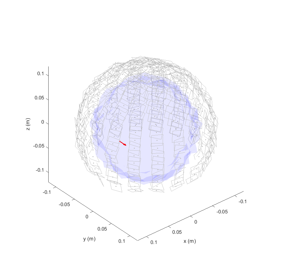
For our reference set-up, we used a simple 1-shell spherical head model of radius 9 cm and conductivity 0.33 S/m with origin located at the center of the sphere, and did a CC BEM forward calculation as described in Sections 2 and 3 to obtain $\bm{\phi}$. The BEM method was implemented using the Matlab library as provided in [35]. The spherical surface was triangulated into 1280 triangles (642 vertices), and 4 dipole sources with varying depths located at $(2,0,0)$ cm, $(4,0,0)$ cm, $(6,0,0)$ cm, and $(8,0,0)$ cm were specified. All the dipoles had a moment of $(0,10,0)$ nAm. To simulate inaccurate mesh modeling to obtain $\bm{\phi}^{\prime}$, the vertices of the spherical mesh were randomly perturbed radially up to 2%, 4%, 6%, 8% and 10% relative to the 9 cm radius.

The sensor array that we used consisted of 324 square magnetometer pick-up loops with side length 2.1 cm all with non-radial orientations (to avoid linear dependence of the SSS basis [38]), uniformly arranged on a spherical shell up to $\pi/6$ below the $z=0$ plane. It has been shown in [40] that a 9-point cubature approximation yields accurate calculations for the sensor distances of 10 cm to 15 cm that we considered, thus we used a 9-point cubature approximation for the calculation of signal vectors in this paper. Figure 1 illustrates the sensor, head, and source setup as described above.

The averaged results over 100 forward calculations with this random vertex perturbation setup is presented in the following sections.

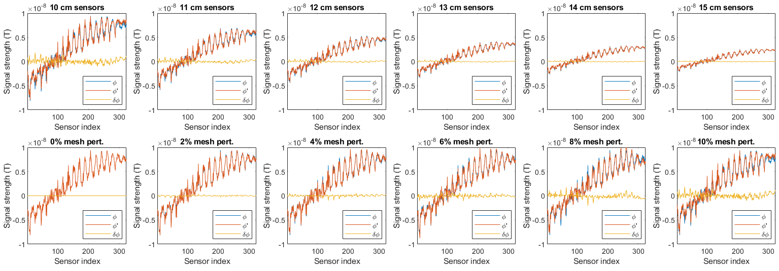
First, we investigate how the error due to BEM mesh inaccuracy varies according to sensor array distance using equation (33). The sensor array radii were set to be from 10 cm to 15 cm, in increments of 1 cm (i.e. 1 cm to 6 cm from the surface of a 9 cm head model) and the signal was assumed the be noiseless. Figure 2 shows that for all the source distances considered, as sensor array distance increases, the subspace angle between the reference signal $\bm{\phi}$ and perturbed signal $\bm{\phi}^{\prime}$ decreases, indicating decreasing relative effects of mesh boundary inaccuracies as sensor array distance from the head increases. Moreover, smaller perturbations to the head model resulted in smaller subspace angles for a given sensor array distance when compared to higher perturbations as expected. These results may also be visually seen via plots of $\bm{\phi}$ and $\bm{\phi}^{\prime}$ explicitly; we show this in Figure 3 with the 2 cm source case across the various sensor distances and mesh perturbations for one of the 100 random mesh perturbation realizations.

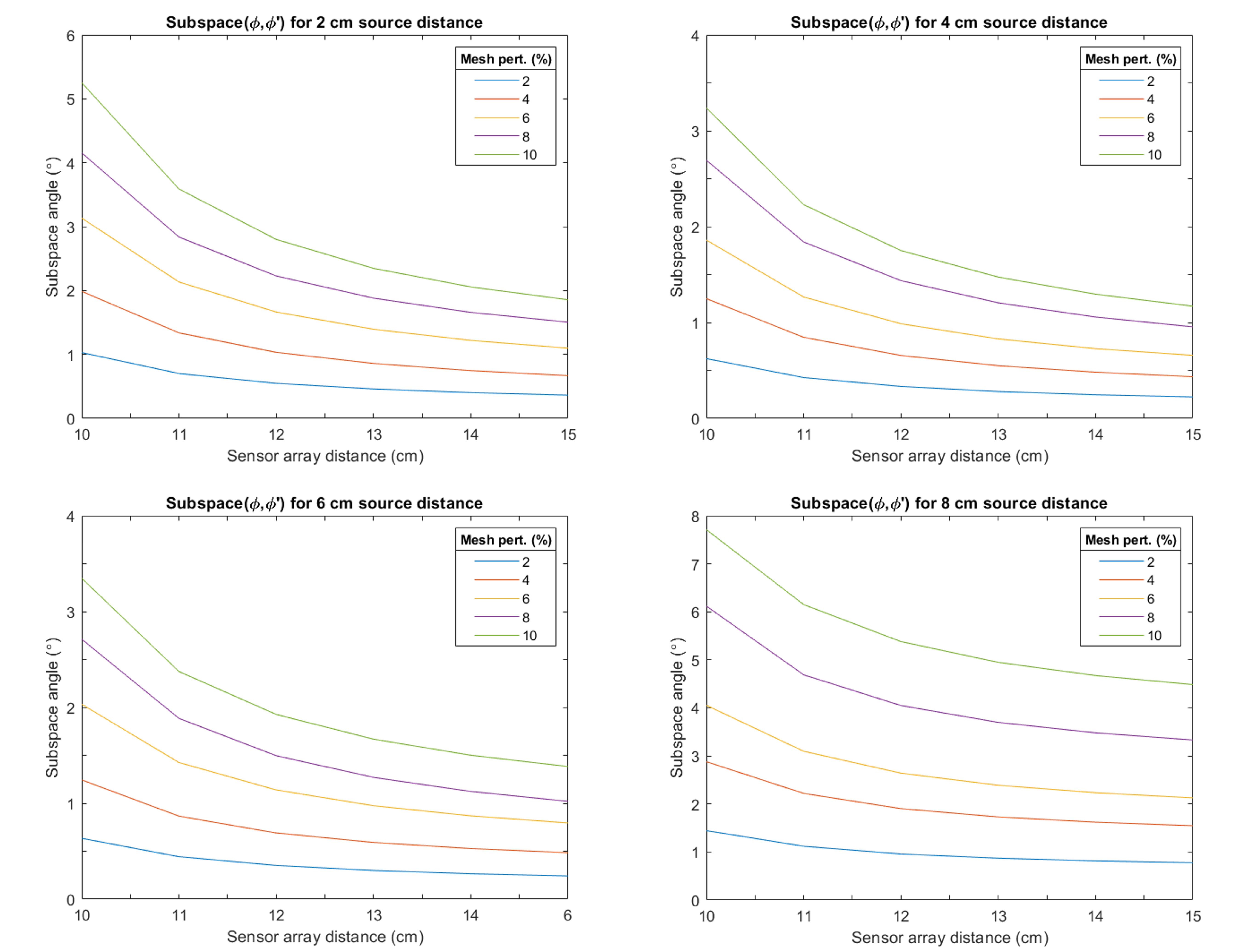
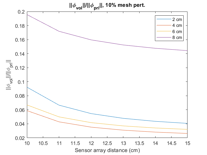
An interesting observation is that from the 2 cm source case to the 4 cm and 6 cm source cases, the subspace angle decreases before increasing again in the 8 cm source case; i.e. there is a “turnaround” point in subspace angle as a function of source distance. This may be explained by the fact that for deeper and superficial sources, the ratio between the volume current contribution to the primary current contribution is higher than for sources that lie between them. For all mesh perturbation cases, 4 cm and 6 cm sources have the lowest volume-to-primary current contributions to the signal as compared to the 2 cm and 8 cm sources. Figure 4 illustrates this for the 10% mesh perturbation case. This may be explained qualitatively by the fact that the 2 cm deep primary source has a low signal strength due to its larger source-to-sensor distance, and hence has a low volume-to-primary current contribution to the signal. The superficial 8 cm source has a small source-to-sensor distance, and hence measures a larger volume current contribution, resulting in the higher volume-to-primary current contribution to the signal. As mentioned previously, all signal errors result from errors in the volume contribution portion only, i.e. $\delta\phi=\delta\bm{\phi}_{vol}$. Thus, the higher volume contribution relative to the primary contribution implies higher signal errors given a same amount of mesh perturbation (equivalently, volume current perturbation) for the 2 cm and 8 cm source cases, hence explaining the “turnaround” point of the subspace angles at some source distance in between them.

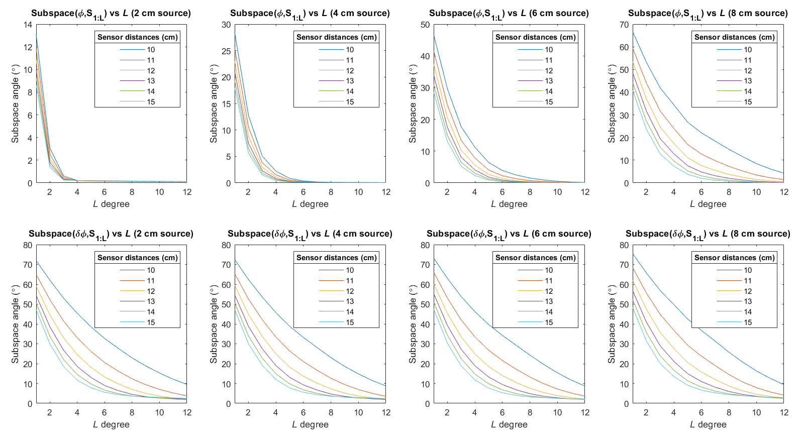
Next, we determine if the additive error of the signal vector, $\delta\bm{\phi}$, may be explained by increasing orders of $l=L$ degree truncation, and if $\delta\bm{\phi}$ varies according to sensor distances. First, we show that the unperturbed signal may be explained to a large extent with $L=12$ degree truncation for all the sensor array distances that we considered. This is shown in the first row of plots in Figure 5; the subspace angle with $\textbf{S}_{1:L}$ decays to become nearly zero at $L=12$ for all source distances. As expected, closer sensor array distances have higher subspace angles than further sensor arrays, which agrees with Figure 2.

From the second row of plots in Figure 5 however, we see that despite the total signal $\bm{\phi}$ being well-explained at $L=12$, the signal errors $\delta\bm{\phi}$ which consist mostly of higher frequency components require a higher $L$ truncation to explain the signal for all source distances. The subspace angle still decreases for increased $l$ degree truncation as expected (since $\delta\phi=\delta\phi_{vol}$ are still volume current contributions), and the subspace angles are smaller for increased sensor array distances. However, the angles are much higher than those of the total signal $\bm{\phi}$, indicating that higher spatial frequency components are affected more by inaccurate mesh modeling. This is because a higher $l$ degree truncation required to fully explain the additive signal error $\delta\bm{\phi}$ of closer sensor arrays indicates that their $\delta\bm{\phi}$ has a more spatially complex pattern with higher spatial frequency components. This higher spatial complexity is due to the fact that higher spatial frequency components decay quickly with increasing distance, hence by placing sensors closer to the source, these components can be captured to give higher resolution of the signal error $\delta\bm{\phi}$. Note that Figure 5 is for the case where the vertices of the mesh was perturbed radially up to 10%. The plots for the different mesh perturbations are similar, hence we present just the 10% case here.

From our results above which considers the noiseless signal case, the signal vector suffers from higher inaccuracies for closer sensor arrays due to the larger errors in their higher spatial frequency components. Deep and superficial sources also had higher signal inaccuracies due to a higher volume current contribution relative to primary currents. Here, we investigate if these observations will be seen in the form of source localization errors as well. The source localization procedure was done via a standard ECD fit using the “fit_dipole” function in MNE-Python 1.0 [13, 14]. The forward model here was computed using LC BEM however, as it is currently the only solving method implemented in MNE-Python.

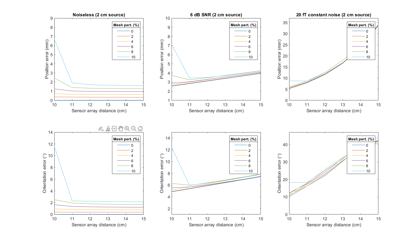
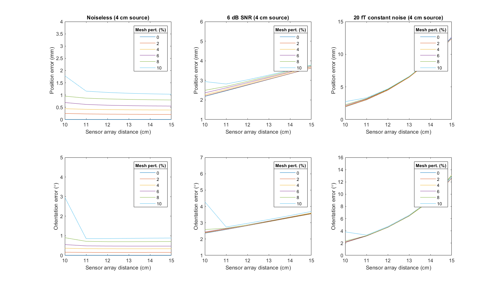
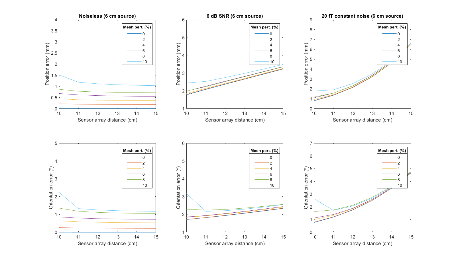
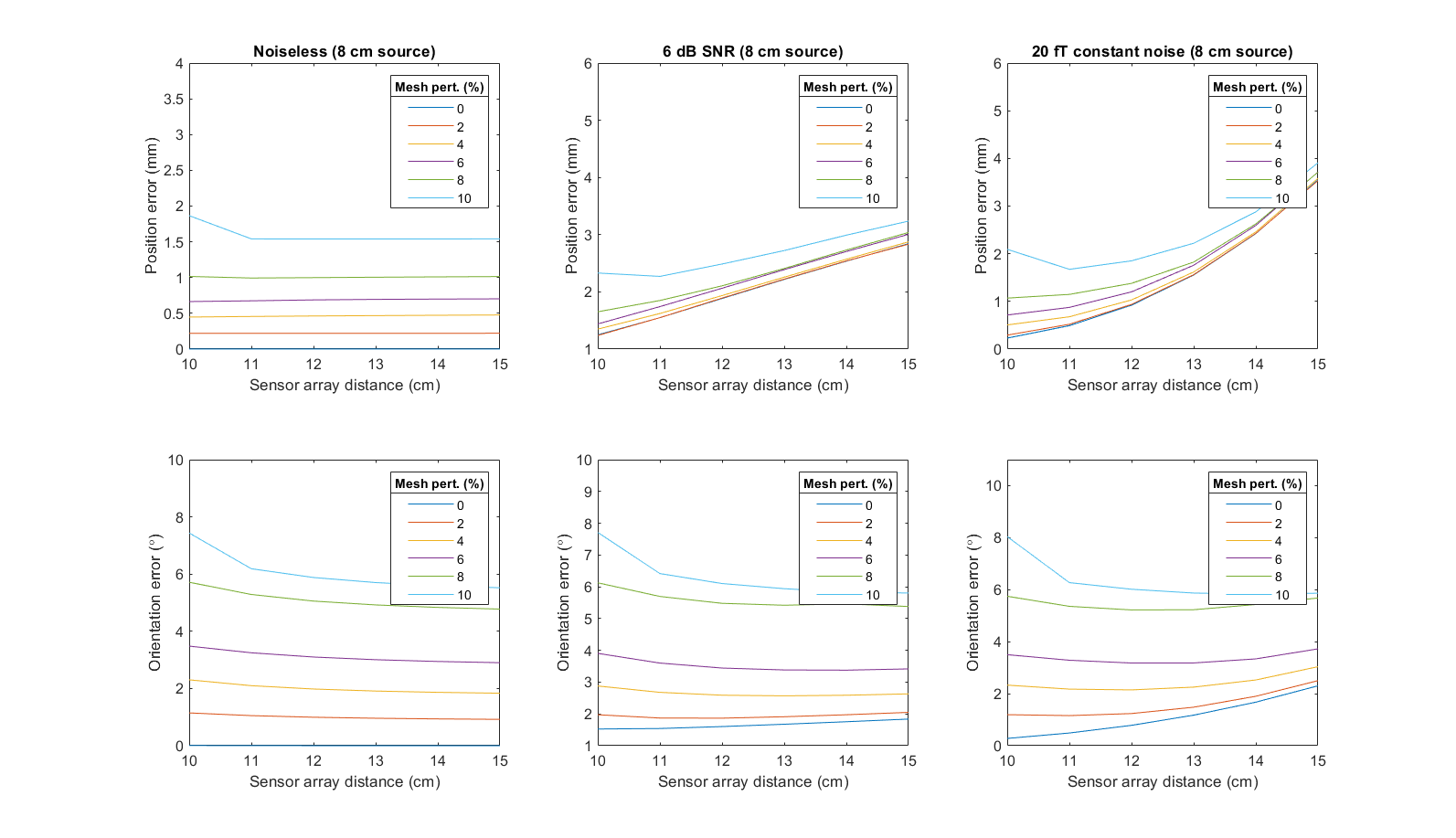
The results for the noiseless case are shown in the first columns of Figures 6, 7, 8 and 9, which correspond to the 2 cm, 4 cm, 6 cm and 8 cm source case respectively. Indeed, in the noiseless case, source localization and orientation errors are largest for closer sensor arrays, as well as deep and superficial sources for a fixed mesh perturbation. These observations are in agreement with the result for signal errors as presented above.

However, the primary motivation to move sensors closer to the head is because closer sensors have the potential to give more accurate source localization results due to higher SNR as mentioned in the introduction. The definition of SNR (with units of decibels) used in MNE-Python 1.0 follows that of Goldenholz [12],

$\displaystyle\text{SNR}=10\log\left\lfloor\frac{q^{2}}{N}\sum_{j=1}^{N}\frac{\phi_{j}^{2}}{s_{j}^{2}}\right\rfloor$

(38)

where $q$ is the source strength, $N$ is the total number of sensors on the sensor array, $\phi_{j}$ is the signal on sensor $j$ and $s_{j}^{2}$ is the noise variance on sensor $j$. We thus introduced various noise levels to determine the noise level at which the effect of having more accurate source localization due to higher SNR of closer sensors outweighs the effect of less accurate source localization due to the higher errors of the high frequency components of the noiseless signal. We found that this occurred at a SNR of around 6 dB (the sensor noise was varied to force a 6 dB SNR for a varying sensor array distances); the localization and orientation errors began to increase as sensor array distances increased at around an SNR of 6 dB. This is shown in the second column of Figures 6, 7, 8 and 9. The rightmost column of Figures 6, 7, 8 and 9 show that for an SNR greater than 6 dB, in this case a constant 20 fT noise level, then there is an improvement in source localization for closer sensor arrays. This means that a higher SNR allowing for better source localization resolutions outweighs the effects of BEM errors for noisy signals with SNR above approximately 6 dB.

References

- [1] M. Abramowitz and I. Stegun, Handbook of Mathematical Functions with Formulas, Graphs, and Mathematical Tables, Dover, New York, 1964.
- [2] A. Borna, T. R. Carter, A. P. Colombo, Y.-Y. Jau, J. McKay, M. Weisend, S. Taulu, J. M. Stephen and P. D. D. Schwindt, “Non-Invasive Functional-Brain-Imaging with an OPM-based Magnetoencephalography System”, PLoS ONE, vol. 15, no. 1, 2020.
- [3] A. Borna, T. R. Carter, J. D. Goldberg, A. P. Colombo, Y.-Y. Jau, C. Berry, J. McKay, J. Stephen, M. Weisend, and P. D. D. Schwindt, “A 20-channel magnetoencephalography system based on optically pumped magnetometers”, Phys. Med. Biol., vol. 62, no. 23, 2017.
- [4] E. Boto, S. S. Meyer, V. Shah, O. Alem, S. Knappe, P. Kruger, T. M. Fromhold, M. Lim, P. M. Glover, P. G. Morris, R. Bowtell, G. R. Barnes and M. J. Brookes, “A new generation of magnetoencephalography: Room temperature measurements using optically-pumped magnetometers”, NeuroImage, vol. 149, pp. 404-414, 2017.
- [5] M. Dannhauer, B. Lanfer, C. H. Wolters and T. R. Knösche T.R., “Modeling of the human skull in EEG source analysis,” Human Brain Mapping, vol. 32, no. 9, pp. 1383–1399, 2011.
- [6] J. C. de Munck, “A linear discretization of the volume conductor boundary integral equation using analytically integrated elements (electrophysiology application),” IEEE Transactions on Biomedical Engineering, vol. 39, no. 9, pp. 986-990, 1992.
- [7] A. S. Ferguson and G. Stroink, “Factors Affecting the Accuracy of the Boundary Element Method in the Forward Problem – I: Calculating Surface Potentials,” IEEE Transactions on Biomedical Engineering, vol. 44, no. 11, 1997.
- [8] A. S. Ferguson, X. Zhang and G. Stroink, “A Complete Linear Discretization for Calculating the Magnetic Field Using the Boundary Element Method,” IEEE Transactions on Biomedical Engineering, vol. 41, no. 5, 1994.
- [9] G. Fischer, B. Tilg, R. Modre, F. Hanser, B. Messnarz and P. Wach, “Modeling the Wilson Terminal in the Boundary and Finite Element Method,” IEEE Transactions on Biomedical Engineering, vol. 49, no. 3, pp. 217-224, 2002.
- [10] N. G. Gençer and I. O. Tanzer, “Forward problem solution of electromagnetic source imaging using a new BEM formulation with high-order elements,” Physics in Medicine & Biology, vol. 44, no. 9, 1999.
- [11] D. B. Geselowitz, “On Bioelectric Potentials in an Inhomogeneous Volume Conductor,” Biophysical Journal, vol. 7, no. 1, pp. 1-11, 1967.
- [12] D. M. Goldenholz, S. P. Ahlfors, M. S. Hämäläinen, D. Sharon, M. Ishitobi, L. M. Vaina and S. M. Stufflebeam, “Mapping the signal‐to‐noise‐ratios of cortical sources in magnetoencephalography and electroencephalography,” Human Brain Mapping, vol. 30, no. 4, pp. 1077-1086, 2008.
- [13] A. Gramfort, M. Luessi, E. Larson, D. A. Engemann, D. Strohmeier, C. Brodbeck, R. Goj, M. Jas, T. Brooks, L. Parkkonen, and M. S. Hämäläinen. “MEG and EEG data analysis with MNE-Python,” Frontiers in Neuroscience, 7(267):1–13, 2013.
- [14] A. Gramfort, M. Luessi, E. Larson, D. A. Engemann, D. Strohmeier, C. Brodbeck, L. Parkkonen, and M. S. Hämäläinen. “MNE software for processing MEG and EEG data,” NeuroImage, 86:446–460, 2014.
- [15] H. Gunawan, O. Neswan and W. Setya-Budhi, “A Formula for Angles between Subspaces of Inner Product Spaces,” Beiträge zur Algebra und Geometrie, vol. 46, no. 2, 2005.
- [16] M. S. Hämäläinen, R. Hari, R. Ilmoniemi, J. Knuutila and O. V. Lounasmaa, “Magnetoencephalography - theory, instrumentation, and applications to noninvasive studies of the working human brain,” Review of Modern Physics, vol. 65, no. 2, pp. 413-497, 1993.
- [17] M. S. Hämäläinen and J. Sarvas, “Realistic Conductivity Geometry Model of the Human Head for Interpretation of Neuromagnetic Data,” IEEE Transactions on Biomedical Engineering, vol. 36, no. 2,1989.
- [18] R. Hari and A. Puce, MEG-EEG Primer, Oxford University Press, 2017.
- [19] J. Haueisen, C. Ramon, M. Eiselt, H. Brauer, H. Nowak, “Influence of tissue resistivities on neuromagnetic fields and electric potentials studied with a finite element model of the head,” IEEE Transactions on Biomedical Engineering, vol. 44, no. 8, pp 727–735, 1997.
- [20] R, M. Hill, E. Boto, M. Rea, N. Holmes, J. Leggett, L. A. Coles, M. Papastavrou, S. K. Everton, B. A. E. Hunt, D. Sims, J. Osborne, V. Shah, R. Bowtell and M. J. Brookes, “Multi-channel whole-head OPM-MEG: Helmet design and a comparison with a conventional system,” NeuroImage, vol. 219, no. 116995, 2020.
- [21] J. Iivanainen, M. Stenroos and L. Parkkonen, “Measuring MEG closer to the brain: Performance of on-scalp sensor arrays,” NeuroImage, vol. 147, p. 542 - 553, 2017.
- [22] J. Iivanainen, R. Zetter, M. Grön, K. Hakkarainen and L. Parkkonen, “On-scalp MEG system utilizing an actively shielded array of optically-pumped magnetometers,” NeuroImage, vol. 194, p. 244 - 257, 2019.
- [23] R. J. Ilmoniemi and J. Sarvas, Brain signals: Physics and mathematics of MEG and EEG. MIT Press, 2019.
- [24] S. Knappe, T. Sander and L. Trahms, Optically-Pumped Magnetometers for MEG, Springer Verlag, Heidelberg, 2014.
- [25] B. Lanfer, M. Scherg, M. Dannhauer, T. R. Knösche, M. Burger and C. H. Wolters, “Influences of skull segmentation inaccuracies on EEG source analysis,” NeuroImage, vol. 62, no. 1, pp. 418-431, 2012.
- [26] M. S. Lynn and W. P. Timlake, “The numerical solution of singular integral equations of potential theory,” Numerische Mathematik, vol. 11, pp. 77-98, 1968.
- [27] A. J. Mäkinen, R. Zetter, J. Iivanainen, K. C. J. Zevenhoven, L. Parkkonen and R. J. Ilmoniemi, “Magnetic-field modeling with surface currents. Part I. Physical and computational principles of bfieldtools,” Journal of Applied Physics, 063906, 2020.
- [28] J. W. H. Meijs, O. W. Weier, M. J. Peters and A. van Oosterom, “On the Numerical Accuracy of the Boundary Element Method,” IEEE Transactions on Biomedical Engineering, vol. 36, no. 10, 1989.
- [29] G. Nolte, T. Fieseler and G. Curio, “Perturbative analytical solutions of the magnetic forward problem for realistic volume conductors,” Journal of Applied Physics, vol. 89, no. 2360, 2001.
- [30] A. V. Oosterom and J. Strakee, “The Solid Angle of a Plane Triangle,” IEEE Transactions on Biomedical Engineering, vol. BME-30, no. 2, pp. 125-126, 1983.
- [31] C. Phillips, J. Mattout and K. Friston, Forward models for EEG, Academic Press, 2006.
- [32] H. A. Schlitt, L. Heller, R. Aaron, E. Best and D. M. Ranken, “Evaluation of Boundary Element Methods for the EEG Forward Problem: Effects of Linear Interpolation,” IEEE Transactions on Biomedical Engineering, vol. 42, no. 1, 1995.
- [33] M. Stenroos, “The transfer matrix for epicardial potential in a piece-wise homogeneous thorax model: the boundary element formulation,” Physics in Medicine & Biology, vol. 54, no. 18, 2009.
- [34] M. Stenroos and O. Hauk, “Minimum-norm cortical source estimation in layered head models is robust against skull conductivity error,” NeuroImage, vol. 81, pp. 265-272, 2013.
- [35] M. Stenroos, V. Mäntynen and J. Nenonen, “A Matlab library for solving quasi-static volume conduction problems using the boundary element method,” Computer Methods and Programs in Biomedicine, vol. 88, no. 3, pp. 256-263, 2007.
- [36] M. Stenroos and A. Nummenmaa, “Incorporating and Compensating Cerebrospinal Fluid in Surface-Based Forward Models of Magneto- and Electroencephalography,” PLoS ONE, vol. 11, no. 7, 2016.
- [37] G. W. Stewart and J.-G. Sun, Matrix perturbation theory, Academic Press, Boston, 1990.
- [38] S. Taulu and M. Kajola, “Presentation of electromagnetic multichannel data: The signal space separation method,” Journal of Applied Physics, vol. 97, 2005.
- [39] S. Vallaghe and M. Clerc, “A Global Sensitivity Analysis of Three- and Four-Layer EEG Conductivity Models,” IEEE Transactions on Biomedical Engineering, vol. 56, no. 4, pp. 988-995, 2009.
- [40] W.-J. Yeo, Y.-R. Yeo and S. Taulu, “Towards analytical calculation of the magnetic flux measured by magnetometers,” Physics Letters A, vol. 411, 2021.