Efficient Adaptive Detection of Complex Event Patterns
Abstract
Complex event processing (CEP) is widely employed to detect occurrences of predefined combinations (patterns) of events in massive data streams. As new events are accepted, they are matched using some type of evaluation structure, commonly optimized according to the statistical properties of the data items in the input stream. However, in many real-life scenarios the data characteristics are never known in advance or are subject to frequent on-the-fly changes. To modify the evaluation structure as a reaction to such changes, adaptation mechanisms are employed. These mechanisms typically function by monitoring a set of properties and applying a new evaluation plan when significant deviation from the initial values is observed. This strategy often leads to missing important input changes or it may incur substantial computational overhead by over-adapting.
In this paper, we present an efficient and precise method for dynamically deciding whether and how the evaluation structure should be reoptimized. This method is based on a small set of constraints to be satisfied by the monitored values, defined such that a better evaluation plan is guaranteed if any of the constraints is violated. To the best of our knowledge, our proposed mechanism is the first to provably avoid false positives on reoptimization decisions. We formally prove this claim and demonstrate how our method can be applied on known algorithms for evaluation plan generation. Our extensive experimental evaluation on real-world datasets confirms the superiority of our strategy over existing methods in terms of performance and accuracy.
Ilya Kolchinsky
Technion, Israel Institute of Technology
Assaf Schuster
Technion, Israel Institute of Technology
1 Introduction
Real-time detection of complex data patterns is one of the fundamental tasks in stream processing. Many modern applications present a requirement for tracking data items arriving from multiple input streams and extracting occurrences of their predefined combinations. Complex event processing (CEP) is a prominent technology for providing this functionality, broadly employed in a wide range of domains, including sensor networks, security monitoring and financial services. CEP engines represent data items as events arriving from event sources. As new events are accepted, they are combined into higher-level complex events matching the specified patterns, which are then reported to end users.
One of the core elements of a CEP system is the evaluation mechanism. Popular evaluation mechanisms include non-deterministic finite automata (NFAs) [49], evaluation trees [42], graphs [8] and event processing networks (EPNs) [30]. A CEP engine uses an evaluation mechanism to create an internal representation for each pattern to be monitored. This representation is constructed according to the evaluation plan, which reflects the structure of . The evaluation plan defines how primitive events are combined into partial matches. Typically, a separate instance of the internal representation is created at runtime for every potential pattern match (i.e., a combination of events forming a valid subset of a full match).
As an example, consider the following scenario.
Example 1. A system for managing an array of smart security cameras is installed in a building. All cameras are equipped with face recognition software, and periodical readings from each camera are sent in real time to the main server. We are interested in identifying a scenario in which an intruder accesses the restricted area via the main gate of the building rather than from the dedicated entrance. This pattern can be represented as a sequence of three primitive events: 1) camera A (installed near the main gate) detects a person; 2) later, camera B (located inside the building’s lobby) detects the same person; 3) finally, camera C detects the same person in the restricted area.
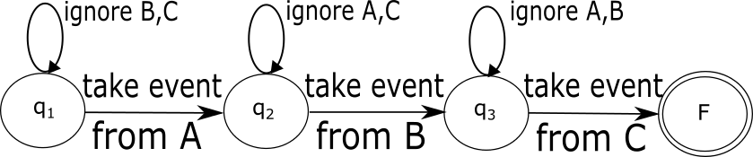

Figure 1LABEL:sub@fig:nfa-no-reordering demonstrates an example of an evaluation mechanism (a non-deterministic finite automaton) for detecting this simple pattern by a CEP engine. This NFA is created according to the following simple evaluation plan. First, a stream of events arriving from camera A is inspected. For each accepted event, the stream of B is probed for subsequently received events specifying the same person. If found, we wait for a corresponding event to arrive from camera C.
Pattern detection performance can often be dramatically improved if the statistical characteristics of the monitored data are taken into account. In the example above, it can be assumed that fewer people access the restricted area than pass through the main building entrance. Consequently, the expected number of face recognition notifications arriving from camera C is significantly smaller than the expected number of similar events from cameras A and B. Thus, instead of detecting the pattern in the order of the requested occurrence of the primitive events (i.e., ), it would be beneficial to employ the “lazy evaluation” principle [36] and process the events in a different order, first monitoring the stream of events from C, and then examining the local history for previous readings of B and A. This way, fewer partial matches would be created. Figure 1LABEL:sub@fig:nfa-with-reordering depicts the NFA constructed according to the improved plan.
Numerous authors proposed methods for defining evaluation plans based on the statistical properties of the data, such as event arrival rates [8, 36, 42, 45]. It was shown that systems tuned according to the a priori knowledge of these statistics can boost performance by up to several orders of magnitude, especially for highly skewed data.
Unfortunately, in real-life scenarios this a priori knowledge is rarely obtained in advance. Moreover, the data characteristics can change rapidly over time, which may render an initial evaluation plan extremely inefficient. In Example 1, the number of people near the main entrance might drop dramatically in late evening hours, making the event stream from camera A the first in the plan, as opposed to the event stream from C.
To overcome this problem, a CEP engine must continuously estimate the current values of the target parameters and, if and whenever necessary, adapt itself to the changed data characteristics. We will denote systems possessing such capabilities as Adaptive CEP (ACEP) systems.
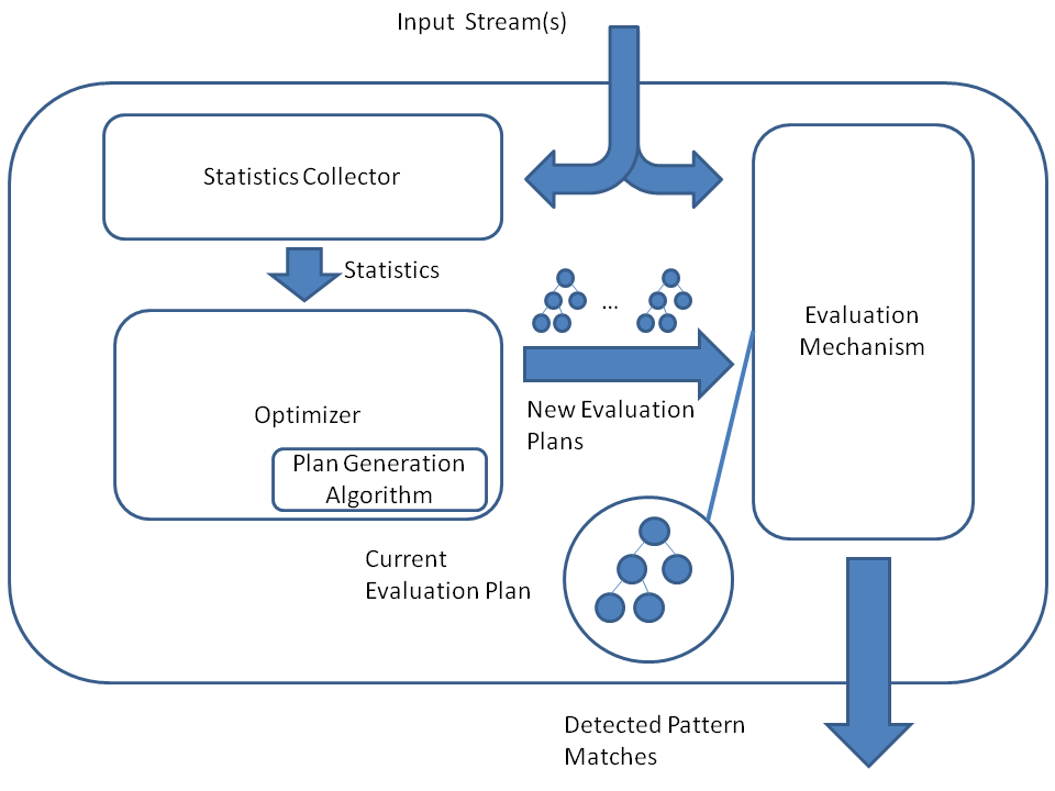
A common structure of an ACEP system is depicted in Figure 2. The evaluation mechanism starts processing incoming events using some initial plan. A dedicated component calculates up-to-date estimates of the statistics (e.g., event arrival rates in Example 1) and transfers them to the optimizer. The optimizer then uses these values to decide whether the evaluation plan should be updated. If the answer is positive, a plan generation algorithm is invoked to produce a new plan (e.g., a new NFA), which is then delivered to the evaluation mechanism to replace the previously employed structure. In Example 1, this algorithm simply sorts the event types in the ascending order of their arrival rates and returns a chain-structured NFA conforming to that order.
Correct decisions by the optimizer are crucial for the successful operation of an adaptation mechanism. As the process of creating and deploying a new evaluation plan is very expensive, we would like to avoid “false positives,” that is, launching reoptimizations that do not improve the currently employed plan. “False negatives,” occurring when an important shift in estimated data properties is missed, are equally undesirable. A flawed decision policy may severely diminish or even completely eliminate the gain achieved by an adaptation mechanism.
The problem of designing efficient and reliable algorithms for reoptimization decision making has been well studied in areas such as traditional query optimization [29]. However, it has received only limited attention in the CEP domain ([36, 42]). In [36], the authors present a structure which reorganizes itself according to the currently observed arrival rates of the primitive events. Similarly to Eddies [13], this system does not adopt a single plan to maintain, but rather generates a new plan for each newly observed set of events regardless of the performance of the current one. The main strength of this method is that it is guaranteed to produce the optimal evaluation plan for any given set of events. However, it can create substantial bottlenecks due to the computational overhead of the plan generation algorithm. This is especially evident for stable event streams with little to no data variance, for which this technique would be outperformed by a non-adaptive solution using a static plan.
The second approach, introduced in [42], defines a constant threshold for all monitored statistics. When any statistic deviates from its initially observed value by more than , plan reconstruction is activated. This solution is much cheaper computationally than the previous one. However, some reoptimization opportunities may be missed.
Consider Example 1 again. Recall that we are interested in detecting the events by the ascending order of their arrival rates, and let the rates for events generated by cameras A, B and C be respectively. Obviously, events originating at A are significantly less sensitive to changes than those originating at B and C. Thus, if we monitor the statistics with a threshold , a growth in C to the point where it exceeds B will not be discovered, even though the reoptimization is vital in this case. Alternatively, setting a value will result in detection of the above change, but will also cause the system to react to fluctuations in the arrival rate of A, leading to redundant plan recomputations.
No single threshold in the presented scenario can ensure optimal operation. However, by removing the conditions involving and monitoring instead a pair of constraints , plan recomputation would be guaranteed if and only if a better plan becomes available.
This paper presents a novel method for making efficient and precise on-the-fly adaptation decisions. Our method is based on defining a tightly bounded set of conditions on the monitored statistics to be periodically verified at runtime. These conditions, which we call invariants, are generated during the initial plan creation, and are constantly recomputed as the system adapts to changes in the input. The invariants are constructed to ensure that a violation of at least one of them guarantees that a better evaluation plan is available.
To the best of our knowledge, our proposed mechanism is the first to provably avoid false positives on reoptimization decisions. It also achieves notably low numbers of false negatives as compared to existing alternatives, as shown by our empirical study. This method can be applied to any deterministic algorithm for evaluation plan generation and used in any stream processing scenario.
The contributions and the structure of this paper can thus be summarized as follows:
• We formally define the reoptimizing decision problem for the complex event processing domain (Section 2).
• We present a novel method for detecting reoptimization opportunities in ACEP systems by verifying a set of invariants on the monitored data characteristics and formally prove that no false positives are possible when this method is used. We also extend the basic method to achieve a balance between computational efficiency and precision (Section 3).
• We demonstrate how to apply the invariant-based method on two known algorithms for evaluation structure creation, the greedy order-based algorithm (an extended version of [36]) and ZStream algorithm [42], and discuss the generalization of these approaches to broader categories of algorithms (Section 4).
• We conduct an extensive experimental evaluation, comparing the invariant-based method to existing state-of-the-art solutions. The results of the experiments, performed on two real-world datasets, show that our proposed method achieves the highest accuracy and the lowest computational overhead (Section 5).
2 Preliminaries
This section presents the notations used throughout this paper, outlines the event detection process in an ACEP system, and provides a formal definition of the reoptimizing decision problem, which will be further discussed in the subsequent sections.
2.1 Notations and Terminology
A pattern recognized by a CEP system is defined by a combination of primitive events, operators, a set of predicates, and a time window. The patterns are formed using declarative specification languages ([49, 24, 28]).
Each event is represented by a type and a set of attributes, including the occurrence timestamp. Throughout this paper we assume that each primitive event has a well-defined type, i.e., the event either contains the type as an attribute or it can be easily inferred from the event attributes using negligible system resources. We will denote the pattern size (i.e., the number of distinct primitive events in a pattern) by .
The predicates to be satisfied by the participating events are usually organized in a Boolean formula. Any condition can be specified on any attribute of an event, including the timestamp (e.g., for supporting multiple time windows).
The operators describe the relations between the events comprising a pattern match. Among the most commonly used operators are sequence (SEQ), conjunction (AND), disjunction (OR), negation (typically marked by ’~’, requires the absence of an event from the stream) and Kleene closure (marked by ’*’, accepts multiple appearances of an event in a specified position). A pattern may include an arbitrary number of operators.
To illustrate the above, consider Example 1 again. We will define three event types according to the identifiers of the cameras generating them: A, B and C. For each primitive event, we will set the attribute person_id to contain a unique number identifying a recognized face. Then, to detect a sequence of occurrences of the same person in three areas in a 10-minute time period, we will use the following pattern specification syntax, taken from SASE [49]:
On system initialization, the pattern declaration is passed to the plan generation algorithm to create the evaluation plan. The evaluation plan provides a scheme for the CEP engine, according to which its internal pattern representation is created. The plan generation algorithm accepts a pattern specification and a set of statistical data characteristic values . It then returns the evaluation plan to be used for detection. If these values are not known in advance, a default, empty , is passed. Multiple plan generation algorithms have been devised, efficiently supporting patterns with arbitrarily complex combinations of the aforementioned operators [35, 42].
In Example 1, contains the arrival rates of event types A, B and C, the evaluation plan is an ordering on the above types, and is a simple sorting algorithm, returning a plan following the ascending order of the arrival rates. The CEP engine then adheres to this order during pattern detection. Another popular choice for a statistic to be monitored is the set of selectivities (i.e., the probabilities of success) of the inter-event conditions defined by the pattern. Examples of plan generation algorithms requiring the knowledge of condition selectivities are presented in Section 4.
The plan generation algorithm attempts to utilize the information in to find the best possible evaluation plan subject to some predefined set of performance metrics, which we denote as . These metrics may include throughput, detection latency, network communication cost, power consumption, and more. For instance, one possible value for in Example 1 is , as processing the events according to the ascending order of their arrival rates was shown to vastly improve memory consumption and throughput of a CEP system [36].
In the general case, we consider to be a computationally expensive operation. We also assume that this algorithm is optimal; that is, it always produces the best possible solution for the given parameters. While this assumption rarely holds in practice, the employed techniques usually tend to produce empirically good solutions.
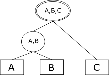
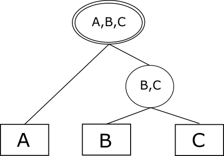
An evaluation plan is not constrained to be merely an order. Figure 3 demonstrates two possible tree-structured plans as defined by ZStream [42]. An evaluation structure following such a plan accumulates the arriving events at their corresponding leaves, and the topology of the internal nodes defines the order in which they are matched and their mutual predicates are evaluated. Matches reaching the tree root are reported to the end users. From this point on, we will denote such plans as tree-based plans, whereas plans similar to the one used for Example 1 will be called order-based plans. While the methods discussed in this paper are independent of the specific plan structure, we will use order-based and tree-based plans in our examples.
2.2 Detection-Adaptation Loop
During evaluation, an ACEP system constantly attempts to spot a change in the statistical properties of the data and to react accordingly. This process, referred to as the detection-adaptation loop, is depicted in Algorithm 1.
The system accepts events from the input stream and processes them using the current evaluation plan. At the same time, the values of the data statistics in are constantly reestimated by the dedicated component (Figure 2), often as a background task. While monitoring simple values such as the event arrival rates is trivial, more complex expressions (e.g., predicate selectivities) require advanced solutions. In this paper, we utilize existing state-of-the-art techniques from the field of data stream processing [14, 27]. These histogram-based methods allow to efficiently maintain a variety of stream statistics over sliding windows with high precision and require negligible system resources.
Opportunities for adaptation are recognized by the reoptimizing decision function , defined as follows:
where is a set of all possible collections of the measured statistic values. accepts the current estimates for the monitored statistic values and decides whether reoptimization is to be attempted111In theory, nothing prevents from using additional information, such as the past and the current system performance. We will focus on the restricted definition where only data-related statistics are considered.. Whenever returns , the detection-adaptation loop invokes . The output of is a new evaluation plan, which, if found more efficient than the current plan subject to the metrics in , is subsequently deployed.
Methods for replacing an evaluation plan on-the-fly without significantly affecting system performance or losing intermediate results are a major focus of current research [29]. Numerous advanced techniques were proposed in the field of continuous query processing in data streams [10, 37, 52]. In our work, we use the CEP-based strategy introduced in [36]. Let be the time of creation of the new plan. Then, partial matches containing at least a single event accepted before are processed according to the old plan , whereas the newly created partial matches consisting entirely of “new” events are treated according to the new plan . Note that since and operate on disjoint sets of matches, there is no duplicate processing during execution. At time (where is the time window of the monitored pattern), the last “old” event expires and the system switches fully to .
In general, we consider the deployment procedure to be a costly operation and will attempt to minimize the number of unnecessary plan replacements.
Input: pattern specification , plan generation algorithm , reoptimizing decision function , initial statistic values
while more events are available:
process incoming events using
estimate current statistic values
if :
if is better than :
apply
2.3 Reoptimizing Decision Problem
The reoptimizing decision problem is the problem of finding a function that maximizes the performance of a CEP system subject to . It can be formally defined as follows: given the pattern specification , the plan generation algorithm , the set of monitored statistics , and the set of performance metrics , find a reoptimizing decision function that achieves the best performance of the ACEP detection-adaptation loop (Algorithm 1) subject to .
In practice, the quality of is determined by two factors. The first factor is the correctness of the answers returned by . Wrong decisions can either fall into the category of false positives (returning when the currently used plan is still the best possible) or false negatives (returning when a more efficient plan is available). Both cases cause the system to use a sub-optimal evaluation plan. The second factor is the time and space complexity of . As we will see in Section 5, an accurate yet resource-consuming implementation of may severely degrade system performance regardless of its output.
We can now analyze the solutions to the reoptimizing decision problem implemented by the adaptive frameworks which we discussed in Section 1. The tree-based NFA [36] defines a trivial decision function , unconditionally returning . In ZStream [42] this functions loops over all values in the input parameter and returns if and only if a deviation of at least is detected.
3 Invariant-Based Method for the Reoptimizing Decision Problem
As illustrated above, the main drawback of the previously proposed decision functions is their coarse granularity, as the same condition is verified for every monitored data property. We propose a different approach, based on constructing a set of fine-grained invariants that reflect the existing connections between individual data characteristics. The reoptimizing decision function will then be defined as a conjunction of these invariants.
In this section, we present the invariant-based decision method and discuss its correctness guarantees, time and space complexity, and possible optimizations.
3.1 Invariant Creation
A decision invariant (or simply invariant) will be defined as an inequality of the following form:
where are sets of the monitored statistic values and are arbitrary functions.
We are interested in finding a single invariant for each building block of the evaluation plan in current use. A building block is defined as the most primitive, indivisible part of a plan. An evaluation plan can then be seen as a collection of building blocks. For instance, the plan for detecting a sequence of three events of types A, B and C, which we discussed in Example 1, is formed by the following three blocks:
-
1.
“Accept an event of type C”;
-
2.
“Scan the history for events of type B matching the accepted C”;
-
3.
“Scan the history for events of type A matching the accepted C and B”.
In general, in an order-based plan, each step in the selected order will be considered a block, whereas for tree-based plans a block is equivalent to an internal node.
We know that the specific plan from the above example was chosen because the plan generation algorithm sorts the event types according to their arrival rates. If, for instance, the rate of B exceeded that of A, the second block would have been “Scan the history for events of type A matching the accepted C” and the third would also have changed accordingly. In other words, the second block of the plan is so defined because, during the run of , the condition was at some point checked, and the result of this check was positive. Following the terminology defined above, in this example consists of all valid arrival rate values and are trivial functions, i.e., .
We will denote any condition (over the measured statistic values) whose verification has led the algorithm to include some building block in the final plan as a deciding condition. Obviously, no generic method exists to distinguish between a deciding condition and a regular one. This process is to be applied separately on any particular algorithm based on its semantics. In our example, assume that the arrival rates are sorted using a simple min-sort algorithm, selecting the smallest remaining one at each iteration. Then, any direct comparison between two arrival rates will be considered a deciding condition, as opposed to any other condition which may or may not be a part of this algorithm’s implementation.
When is invoked on a given input, locations can be marked in the algorithm’s execution flow where the deciding conditions are verified. We will call any actual verification of a deciding condition a block-building comparison (BBC). For instance, assume that we start executing our min-sort algorithm and a deciding condition is verified. Further assume that is smaller than . Then, this verification is a BBC associated with the building block “Accept an event of type C first”, because, unless this deciding condition holds, the block will not be included in the final plan. This will also be the case if is subsequently verified and is smaller. If is smaller, the opposite condition, ,/ becomes a BBC associated with a block “Accept an event of type B first”. Overall, BBCs take place during the first min-sort iteration, during the second iteration, and so forth.
In general, for each building block of any evaluation plan, we can determine a deciding condition set (DCS). A DCS of consists of all deciding conditions that were actually checked and satisfied by BBCs belonging to as explained above. Note that, by definition, the intersection of two DCSs is always empty. In our example, assuming that the blocks listed above are denoted as , the DCSs are as follows:
As long as the above conditions hold, no other evaluation plan can be returned by . On the other hand, if any of the conditions is violated, the outcome of will result in generating a different plan. If we define the decision function as a conjunction of the deciding condition sets, we will recognize situations in which the current plan becomes sub-optimal with high precision and confidence.
However, verifying all deciding conditions for all building blocks is very inefficient. In our simple example, the total number of such conditions is quadratic in the number of event types participating in the pattern. For more complicated plan categories and generation algorithms, this dependency may grow to a high-degree polynomial or even become exponential. Since the adaptation decision is made during every iteration of Algorithm 1, the overhead may not only decrease the system throughput, but also negatively affect the response time.
To overcome this problem, we will constrain the number of conditions to be verified by to one per building block. For each deciding condition set , we will determine the tightest condition, that is, the one that was closest to being violated during plan generation. This tightest condition will be selected as an invariant of the building block . In other words, we may alternatively define an invariant as a deciding condition selected for actual verification by out of a DCS. More formally, given a set,
we will select a condition minimizing the expression
as an invariant of the building block .
In the example above, the invariant for is , since we know that , and therefore . It is clear that is a tighter bound for the value of than .
To summarize, the process of invariant creation proceeds as follows. During the run of on the current set of statistics , we closely monitor its execution. Whenever a block-building comparison is detected for some block , we add the corresponding deciding condition to the DCS of . After the completion of , the tightest condition of each DCS is extracted and added to the invariant list.
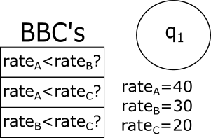
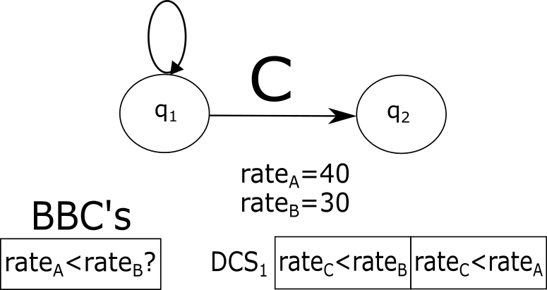
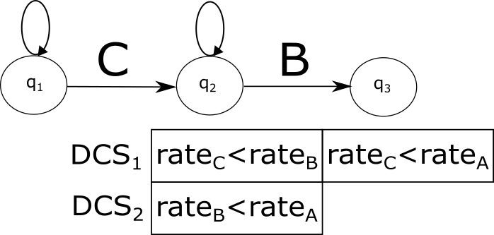
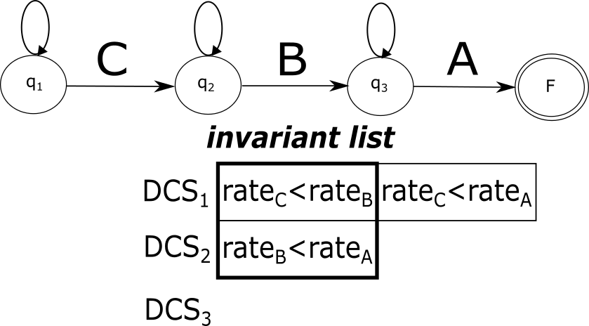
Figure 4 demonstrates the invariant creation process applied on the pattern from Example 1 and the rate-sorting algorithm discussed above. Each subfigure depicts a different stage in the plan generation and presents the DCSs and the BBCs involved at this stage.
As discussed above, this generic method has to be adapted to any specific implementation of . This is trivially done for any which constructs the solution plan in a step-by-step manner, selecting and appending one building block at a time. However, for algorithms incorporating other approaches, such as dynamic programming, it is more challenging to attribute a block-building comparison to a single block of the plan. In Section 4, we will exemplify this process on two algorithms taken from the previous work in the field and discuss its applicability on broader algorithm categories.
3.2 Invariant Verification and Adaptation
During the execution of the detection-adaptation loop (Algorithm 1), traverses the list of invariants built as described above. It returns if a violated invariant was found (according to the current statistic estimates) and otherwise. This list is sorted according to the order of the respective building blocks in the evaluation plan. In Example 1, first the invariant will be verified, followed by . The reason is that an invariant implicitly assumes the correctness of the preceding invariants (e.g., assumes that holds; otherwise, it should have been changed to ). For tree-based plans, the verification proceeds in a bottom-up order. For example, for the tree plan displayed in Figure 3LABEL:sub@fig:zstream-abc-left, the order is .
If a violation of an invariant is detected, is invoked to create a new evaluation plan. In this case, the currently used invariants are invalidated and a new list is created following the process described above. Subsequent verifications performed by are then based on the new invariants.
Assuming that any invariant can be verified in constant time and memory, the complexity of using the invariant-based method is , where is the number of the building blocks in an evaluation plan. This number is bounded by the pattern size (the number of event types participating in a pattern) for both order-based and tree-based plans. To guarantee this result, an application of the invariant-based method on a specific implementation of has to ensure that the verification of a single invariant is a constant-time operation, as we exemplify in Section 4.
3.3 Correctness Guarantees and the K-invariant Method
We will now formally prove that the invariant-based method presented above guarantees that no false positive detections will occur during the detection-adaptation loop.
Theorem 1
Let be a reoptimizing decision function implemented according to the invariant-based method. Let be a deterministic plan generation algorithm in use and let be the currently employed plan. Then, if at some point during execution returns , the subsequent invocation of will return a plan , such that .
By definition, if returns , then there is at least one invariant whose verification failed, i.e., its deciding condition does not hold anymore. Let be the first such condition, and let be the building block such that (recall that there is only one such ). Then, by determinism of and by the ordering defined on the invariants, the new run of will be identical to the one that produced until the block-building comparison that checks . At that point, by definition of the block-building comparison, the negative result of validating will cause to reject as the current building block and select a different one, thus producing a plan , which is different from .
Since we assume to always produce the optimal solution, the above result can be extended.
Corollary 1
Let be an invariant-based reoptimizing decision function and let be a deterministic plan generation algorithm in use. Then, if at some point during execution returns , the subsequent invocation of will return a plan that is more efficient than the currently employed one.
Note that the opposite direction of Theorem 1 does not hold. It is still possible that a more efficient evaluation plan can be deployed, yet this opportunity will not be detected by because we only pick a single condition from each deciding condition set (see Section 4.2 for an example). If we were to include the whole union of the above sets in the invariant set, even stronger guarantees could be achieved, as stated in the following theorem.
Theorem 2
Let be a reoptimizing decision function implemented according to the invariant-based method, with all conditions from all DCSs included in the invariant set. Let be a deterministic plan generation algorithm in use and let be the currently employed plan. Then, if and only if at some point during the execution returns , the subsequent invocation of will return a plan , such that .
The first direction follows immediately from Theorem 1. For the second direction, let and let be the first building blocks that differ in and . By ’s determinism, there exist s. t.
as otherwise there would be no way for to deterministically choose between and . Since was created by using the currently estimated statistic values, we can deduce that holds. Consequently, does not hold. By the assumption that all deciding conditions are included in the invariant set, will necessarily detect this violation, which completes the proof.
The above result shows that greater precision can be gained if we do not limit the number of monitored invariants per building block. However, as discussed above, validating all deciding conditions may drastically increase the adaptation overhead.
The tradeoff between performance and precision can be controlled by introducing a new parameter , defined as the maximal number of conditions from a deciding set to select as invariants. We will refer to the method using a specific value of as the K-invariant method, as opposed to the basic invariant method discussed above. Note that the 1-invariant method is equivalent to the basic one. The K-invariant method becomes more accurate and more time-consuming for higher values of . The total number of the invariants in this case is at most .
3.4 Distance-Based Invariants
By Corollary 1, it is guaranteed that a new, better evaluation plan will be produced following an invariant violation. However, the magnitude of its improvement over the old plan is not known. Consider a scenario in which two event types in a pattern have very close arrival rates. Further assume that there are slight oscillations in the rates, causing the event types to swap positions periodically when ordered according to this statistic. If an invariant is defined comparing the arrival rates of these two types, then will discover these minor changes and two evaluation plans with little to no difference in performance will be repeatedly produced and deployed. Although not a “false positive” by definition, the overhead implied by this situation may exceed any benefit of using an adaptive platform.
To overcome this problem, we will introduce the notion of the minimal distance , defined as the smallest relative difference between the two sides of the inequality required for an invariant to be considered as violated. That is, given a deciding condition
we will construct the invariant to be verified by as follows:
The experimental study in Section 5 demonstrates that a correctly chosen leads to a significant performance improvement over the basic technique. However, finding a sufficiently good is a difficult task, as it depends on the data, the type of statistics, the invariant expression, and the frequency and magnitude of the runtime changes. We identify the following directions for solving this problem:
-
1.
Parameter scanning: empirically checking a range of candidate values to find the one resulting in the best performance. This method is the simplest, but often infeasible in real-life scenarios.
-
2.
Data analysis methods: calculating the distance by applying a heuristic rule on the currently available statistics can provide a good estimate in some cases. For instance, we can monitor the initial execution of the plan generation algorithm and set as the average obtained relative difference between the sides of a deciding condition or, more formally:
The effectiveness of this approach depends on the distribution and the runtime behavior of the statistical values. Specifically, false positives may occur when the values are very close and the changes are frequent. Still, we expect it to perform reasonably well in the common case. This technique can also be utilized to produce a starting point for parameter scanning.
-
3.
Meta-adaptive methods: dynamically tuning on-the-fly to adapt it to the current stream statistics. This might be the most accurate and reliable solution. We start with some initial value, possibly obtained using the above techniques. Then, as invariants are violated and new plans are computed, modify to prevent repeated reoptimization attempts when the observed gain in plan quality is low. An even higher precision can be achieved by additionally utilizing fine-grained per-invariant distances. This advanced research direction is a subject for our future work.
We implement and experimentally evaluate the first two approaches in Section 5.
3.5 Tightest Conditions Selection Strategy
In Section 3.1 we explained that, given a DCS for a block , the condition to be included in the invariant set is the one with the smallest difference between the sides of the inequality (according to the currently observed values of the statistics). The intention of this approach is to pick a condition most likely to be violated later. This, however, is merely a heuristic. In many cases, there may be no correlation at all between the difference of the currently observed values and the probability of the new values to violate the inequality. Hence, this selection strategy may result in suboptimal invariant selection.
However, sometimes the information regarding the expected variance of a data property is either given in advance or can be calculated to some degree of precision and even approximated on-the-fly [14]. In these cases, a possible optimization would be to explicitly calculate the violation probability of every deciding condition and use it as a metric for selecting an invariant from a deciding condition set.
4 Applications of the Invariant-Based Method
In Section 3, we presented a generic method for defining a reoptimizing decision function as a list of invariants. As we have seen, additional steps are required in order to apply this method to a specific choice of the evaluation plan structure and the plan generation algorithm. Namely, the following should be strictly defined: 1)what is considered a building block in a plan; 2)what is considered a block-building comparison in ; 3)how we associate a BBC with a building block. Additionally, efficient verification of the invariants must be ensured. In this section, we will exemplify this process on two plan-algorithm combinations taken from previous works in the field. The experimental study in Section 5 will also be conducted on these adapted algorithms. We also discuss how the presented techniques can be generalized to several classes of algorithms.
4.1 Greedy Algorithm for Order-Based Plans
The greedy heuristic algorithm based on cardinalities and predicate selectivities was first described in [47] for creating left-deep tree plans for join queries. The algorithm supports all operators described in Section 2.1 and their arbitrary composition. Its basic form, which we describe shortly, only targets conjunction and sequence patterns of arbitrary complexity. Support for other operators and their composition is implemented by either activating transformation rules on the input pattern or applying post-processing steps on the generated plan (e.g., to augment it with negated events). As these additional operations do not affect the application of the invariant-based method, we do not describe them here. The reader is referred to [35] for more details.
The algorithm proceeds iteratively, selecting at each step the event type which is expected to minimize the overall number of partial matches (subsets of valid pattern matches) to be kept in memory. At the beginning, the event type with the lowest arrival rate (multiplied by the selectivities of any predicates possibly defined solely on this event type) is chosen. At each subsequent step , the event type to be selected is the one minimizing the expression
where stands for the arrival rate of the event type in a pattern, is the selectivity of the predicate defined between the and the event types (equals to 1 if no predicate is defined), are the event types selected during previous steps, and is the candidate event type for the current step. Since a large part of this expression is constant when selecting , it is sufficient to find an event type, out of those still not included in the plan, minimizing the expression
Input: event types , arrival rates , inter-event predicate selectivities
Output: order-based evaluation plan
add to
for from 2 to :
add to
return
Algorithm 2 depicts the plan generation process. When all selectivities satisfy , i.e., no predicates are defined for the pattern, this algorithm simply sorts the events in an ascending order of their arrival rates.
We will define a building block for order-based evaluation plans produced by Algorithm 2 as a single directive of processing an event type in a specific position of a plan. That is, a building block is an expression of the form “Process the event type at position in a plan”. Obviously, a full plan output by the algorithm will contain exactly blocks, while a total of blocks will be considered during the run. Deciding conditions created for such a building block will be of the following form:
Here, is an event type which was considered to occupy position at some point but eventually was selected. Note that, while in the worst case the products may contain up to multiplicands, in most cases the number of the predicates defined over the events in a pattern is significantly lower than . Therefore, invariant verification will be executed in near-constant time.
4.2 Dynamic Programming Algorithm for Tree-Based Plans
Input: event types , arrival rates , inter-event predicate selectivities
Output: a tree-based evaluation plan
new two-dimensional matrix of size
for from 1 to :
for from 2 to :
for from 1 to :
for from to :
if
return
The authors of ZStream [42] introduced an efficient algorithm for producing tree-based plans based on dynamic programming (Algorithm 3). The algorithm consists of steps, where during the step the tree-based plans for all subsets of the pattern of size are calculated (for the trees of size 1, the only possible tree containing the lone leaf is assumed). During this calculation, previously memoized results for the two subtrees of each tree are used. To calculate the cost of a tree with the subtrees and , the following formula is used:
where is the cardinality (the expected number of partial matches reaching the root) of , whose calculation depends on the operator applied by the root. For example, the cardinality of a conjunction node is defined as the product of the cardinalities of its operands multiplied by the total selectivity of the conditions between the events in and the events in . That is,
where is a product of all predicate selectivities . Leaf cardinalities are defined as the arrival rates of the respective event types. The reader is referred to [42] for more details.
To apply the invariant-based adaptation method on this algorithm, we will define each internal node of a tree-based plan as a building block. This way, up to blocks will be formed during the run of Algorithm 3, with only included in the resulting plan.
A comparison between the costs of two trees will be considered a block-building comparison for the root of the less expensive tree. The deciding conditions for this algorithm will be thus defined simply as , where are the two compared trees. These comparisons are invoked at each step during the search for the cheapest tree over a given subset of events. For events, the number of candidate trees is , where is the Catalan number. Therefore, picking only one comparison as an invariant and dismissing the rest of the candidates may create a problem of false negatives, and K-invariant method is recommended instead (see discussion in Section 3.3).
The obvious problem with the above definition is that tree cost calculation is a recursive function, which contradicts our constant-time invariant verification assumption. We will eliminate this recursion by utilizing the following observation. In Algorithm 3, all block-building comparisons are performed on pairs of trees defined over the same set of event types. By invariant definition, one of these trees is always a subtree of a plan currently being in use. Recall that invariants on tree-based plans are always verified in the direction from leaves to the root. Hence, if any change was detected in one of the statistics affecting the subtrees of the two compared trees, it would be noticed during verification of earlier invariants. Thus, it is safe to represent the cost of a subtree in an invariant as a constant whose value is initialized to the cost of that subtree during invariant creation (i.e., plan construction).
4.3 General Applicability of the Invariant-Based Method
The approaches described in Sections 4.1 and 4.2 only cover two special cases. Here, we generalize the presented methodologies to apply the invariant-based method to any greedy or dynamic programming algorithm. We also discuss the applicability of our method to other algorithm categories.
A generalized variation of the technique illustrated in Section 4.1 can be utilized for any greedy plan generation algorithm. To that end, a part of a plan constructed during a single greedy iteration should be defined as a building block. Additionally, a conjunction of all conditions evaluated to select a specific block is to be defined as a block-building comparison associated with this block. Since most greedy algorithms require constant time and space for a single step, the complexity requirements for the invariant verification will be satisfied.
Using similar observations, we can generalize the approach described in Section 4.2 to any dynamic programming algorithm. A subplan memoized by the algorithm will correspond to a building block. A comparison between two subplans will serve as a BBC for the block that was selected during the initial run.
In general, the invariant-based method can be similarly adapted to any algorithm that constructs a plan in a deterministic, bottom-up manner, or otherwise includes a notion of a “building block”. To the best of our knowledge, the majority of the proposed solutions share this property.
In contrast, algorithms based on randomized local search (adapted to CEP in [34]) cannot be used in conjunction with the invariant-based method. Rather than building a plan step-by-step, these algorithms start with a complete initial solution and randomly modify it to create an improved version [3] until some stopping condition is satisfied.
5 Experimental Evaluation
In this section, the results of our experimental evaluation are presented. The objectives of this empirical study were twofold. First, we wanted to assess the overall system performance achieved by our approach and the computational overhead implied by its adaptation process as compared to the existing strategies for ACEP systems, outlined in Section 1. Our second goal was to explore how changes in the parameters of our method and of the data characteristics impact the above metrics.
5.1 Experimental Setup
We implemented the two CEP models described in Section 4, the lazy NFA [36] with the greedy order-based algorithm [47] and the ZStream model with tree-based dynamic programming algorithm [42]. We also added support for three adaptation methods (i.e., implementations of ): 1) the unconditional reoptimization method from [36]; 2) the constant-threshold method from [42]; 3) the invariant-based method. To accurately estimate the event arrival rates and predicate selectivities on-the-fly, we utilized the algorithm presented in [27] for maintaining statistics over sliding window.
Since the plan generation algorithms used during this study create plans optimized for maximal throughput, we choose throughput as a main performance metric, reflecting the effectiveness of the above algorithms in the presence of changes in the input. We believe that similar results could be obtained for algorithms targeting any other optimization goal, such as minimizing latency or communication cost.
Two real-world datasets were used in the experiments. For each of them, we created 5 sets of patterns containing different operators (Section 2.1), as follows: (1)sequences; (2)sequences with an event under negation; (3)conjunctions; (4)sequences with an event under Kleene closure; (5)composite patterns, consisting of a disjunction of three shorter sequences. Each set contained 6 patterns of sizes varying from 3 to 8. The details are specified below for each dataset. Our main results presented in this section are averaged over all pattern sets unless otherwise stated. We provide the full description of the specific results obtained for each set in Appendix A.
The first dataset contains the vehicle traffic sensor data, provided by City of Aarhus, Denmark [9] and collected over a period of 4 months from 449 observation points, with 13,577,132 primitive events overall. Each event represents an observation of traffic at the given point. The attributes of an event include, among others, the point ID, the average observed speed, and the total number of observed vehicles during the last 5 minutes. The arrival rates and selectivities for this dataset were highly skewed and stable, with few on-the-fly changes. However, the changes that did occur were mostly very extreme. The patterns for this dataset were motivated by normal driving behavior, where the average speed tends to decrease with the increase in the number of vehicles on the road. We requested to detect the violations of this model, i.e., combinations (sequences, conjunctions, etc., depending on the operator involved) of three or more observations with either an increase or a decline in both the number of vehicles and the average speed.
The second dataset was taken from the NASDAQ stock market historical records [1]. Each record in this dataset represents a single update to the price of a stock, spanning a 1-year period and covering over 2100 stock identifiers with prices updated on a per minute basis. Our input stream contained 80,509,033 primitive events, each consisting of a stock identifier, a timestamp, and a current price. For each stock identifier, a separate event type was defined. In addition, we preprocessed the data to include the difference between the current and the previous price. Contrary to the traffic dataset, low skew in data statistics was observed, with the initial values nearly identical for all event types. The changes were highly frequent, but mostly minor. The patterns to evaluate were then defined as combinations of different stock identifiers (types), with the predefined price differences (e.g., for a conjunction pattern we require ).
All models and algorithms under examination were implemented in Java. All experiments were run on a machine with 2.20 Ghz CPU and 16.0 GB RAM.
5.2 Experimental Results
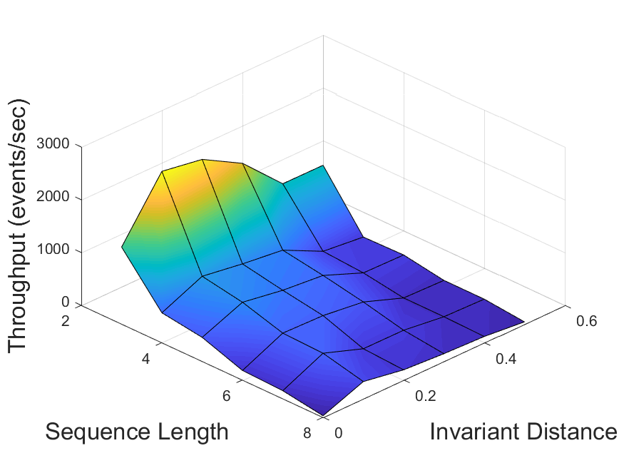
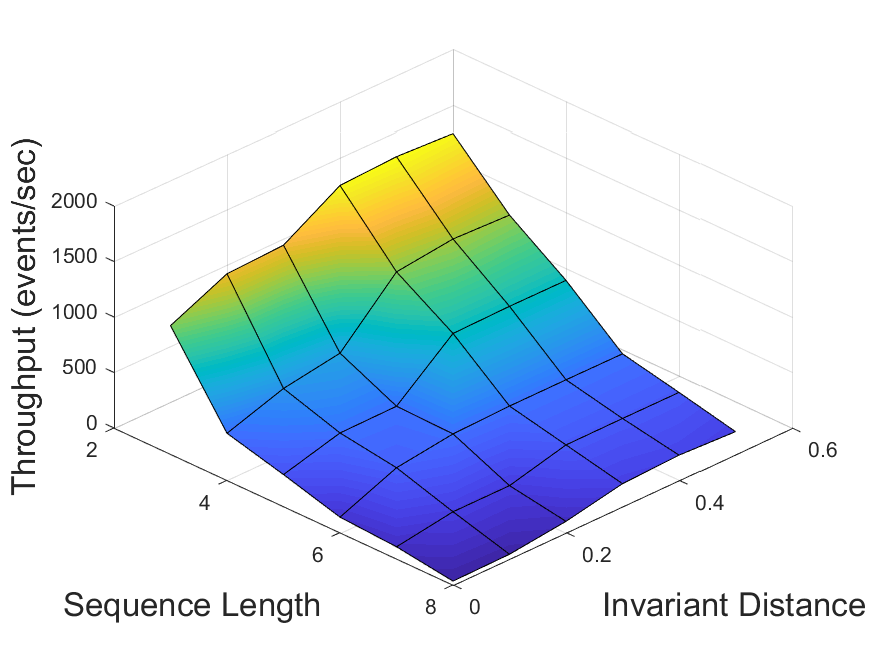
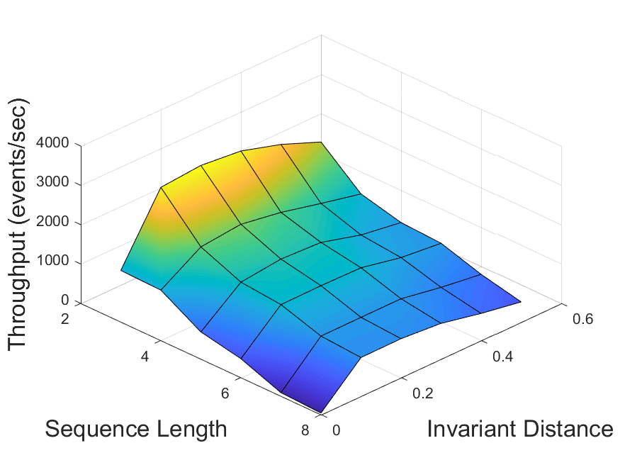
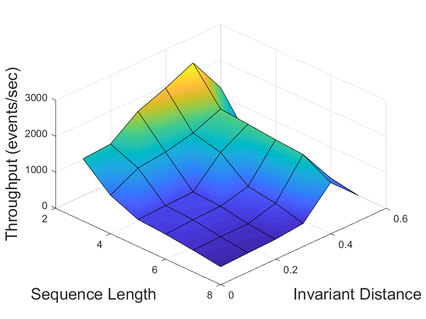
In our first experiment, we evaluated the performance of the invariant-based method for different values of the invariant distance (Section 3.4). In this experiment, only the sequence pattern sets were used. For each of the four possible dataset-algorithm combinations, the system throughput was measured as a function of the tested pattern size and of , with its values ranging from 0 (which corresponds to the basic method) to 0.5. The results are displayed in Figure 5. It can be observed that in each scenario there exists an optimal value , which depends on the data and the algorithm in use, consistently outperforming the other values for all pattern sizes. For distances higher than , too many changes in the statistics are undetected, while the lower values trigger unnecessary adaptations. Overall, the throughput achieved by using invariants with distance is 2 to 25 times higher than that of the basic method ().
Then, we validated the average relative difference method described in Section 3.4 by comparing its output value to (obtained via parameter scanning as described above) for each scenario. The results are summarized in Table 1.
For the traffic dataset, the computed values were considerably close to the optimal ones for patterns of length 6 and above, with precision reaching at least 87% (for ZStream algorithm and pattern length 7) and as high as 92% (Greedy algorithm, length 8). For the stocks dataset, the achieved accuracy was only 31-44%. We can thus conclude that the tested method does not function well in presence of low data skew, matching our expectations from Section 3.4. This highlights the need for developing better solutions, which is the goal of our future work.
It can also be observed that for all dataset-algorithm combinations the prevision of the average relative difference method increases with pattern size. We estimate that the scalability of this method would further increase for even larger patterns.
| Dataset | Algorithm | Pattern Size | |||
|---|---|---|---|---|---|
| Traffic | Greedy | 4 | 0.1695 | 0.1 | 0.59 |
| Traffic | Greedy | 5 | 0.1211 | 0.1 | 0.826 |
| Traffic | Greedy | 6 | 0.1163 | 0.1 | 0.86 |
| Traffic | Greedy | 7 | 0.0909 | 0.1 | 0.909 |
| Traffic | Greedy | 8 | 0.0921 | 0.1 | 0.921 |
| Traffic | ZStream | 4 | 0.9153 | 0.4 | 0.437 |
| Traffic | ZStream | 5 | 0.6514 | 0.4 | 0.614 |
| Traffic | ZStream | 6 | 0.4551 | 0.4 | 0.879 |
| Traffic | ZStream | 7 | 0.4581 | 0.4 | 0.873 |
| Traffic | ZStream | 8 | 0.4464 | 0.4 | 0.896 |
| Stocks | Greedy | 4 | 0.0556 | 0.2 | 0.278 |
| Stocks | Greedy | 5 | 0.0268 | 0.2 | 0.134 |
| Stocks | Greedy | 6 | 0.0661 | 0.2 | 0.331 |
| Stocks | Greedy | 7 | 0.0818 | 0.2 | 0.409 |
| Stocks | Greedy | 8 | 0.0866 | 0.2 | 0.443 |
| Stocks | ZStream | 4 | 0.095 | 0.4 | 0.24 |
| Stocks | ZStream | 5 | 0.102 | 0.4 | 0.255 |
| Stocks | ZStream | 6 | 0.1231 | 0.4 | 0.308 |
| Stocks | ZStream | 7 | 0.1563 | 0.4 | 0.391 |
| Stocks | ZStream | 8 | 0.1206 | 0.4 | 0.304 |
Next, we performed an experimental comparison of all previously described adaptation methods. The comparison was executed separately for each dataset-algorithm combination. For the invariant-based method, the values obtained during the previous experiment were used. For the constant-threshold method, an optimal threshold was empirically found for each of the above combinations using a similar series of runs.
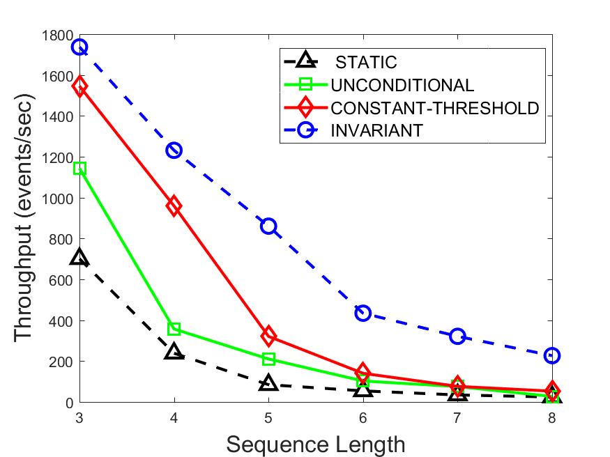
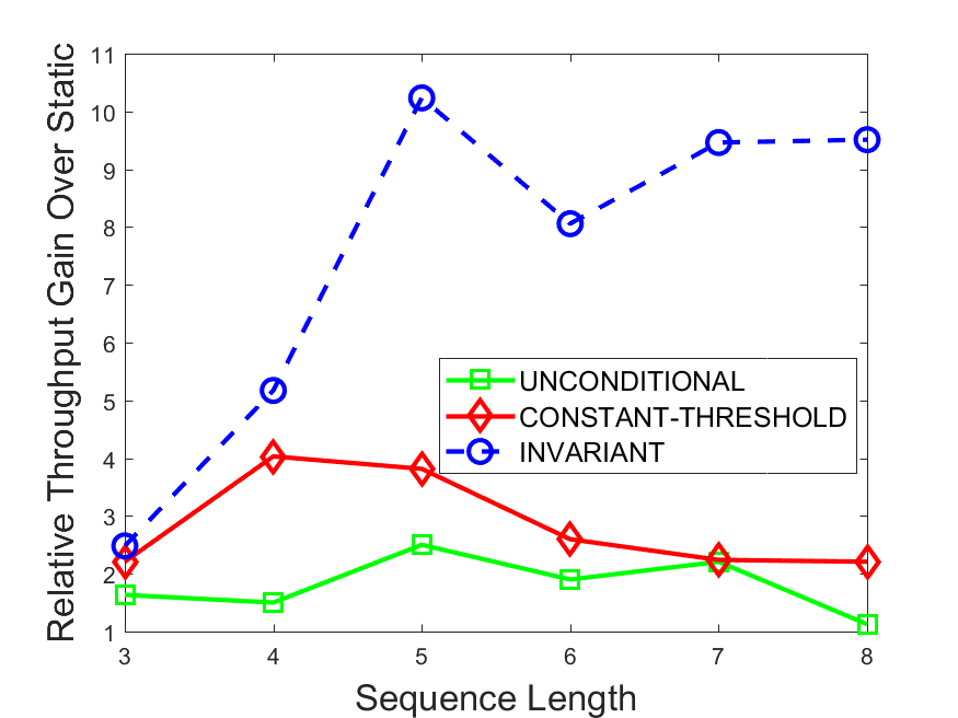
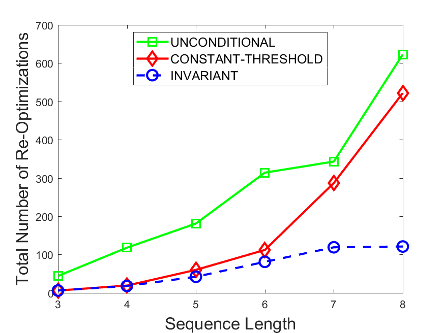
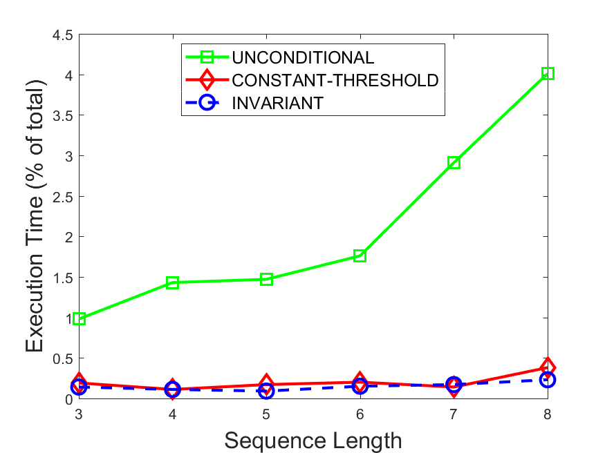
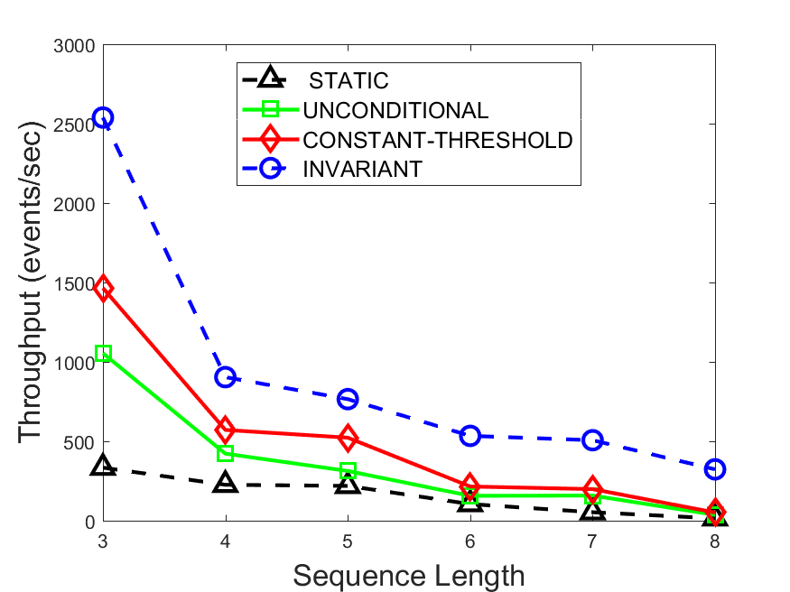
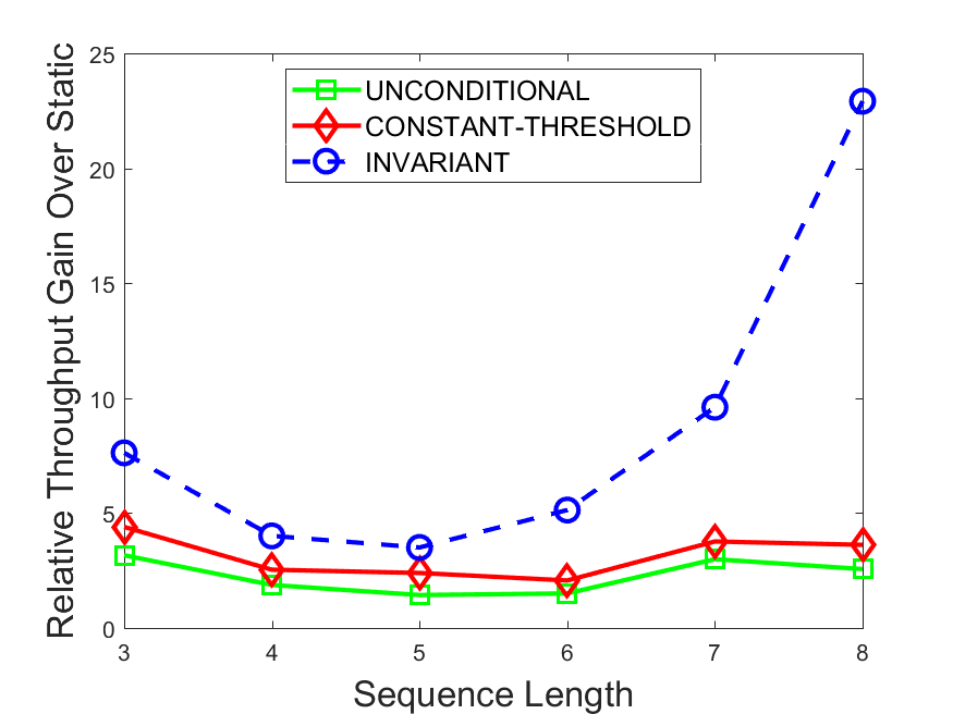
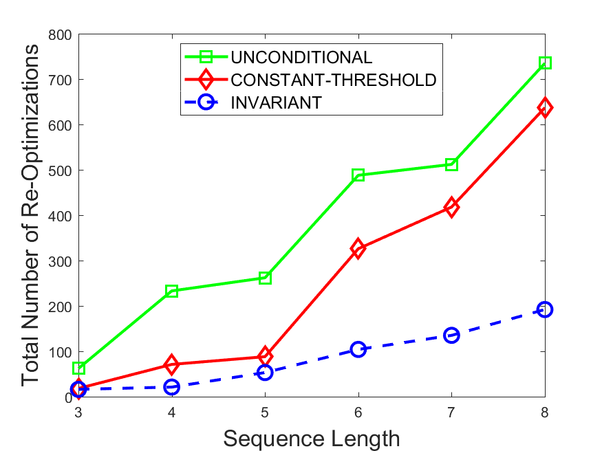
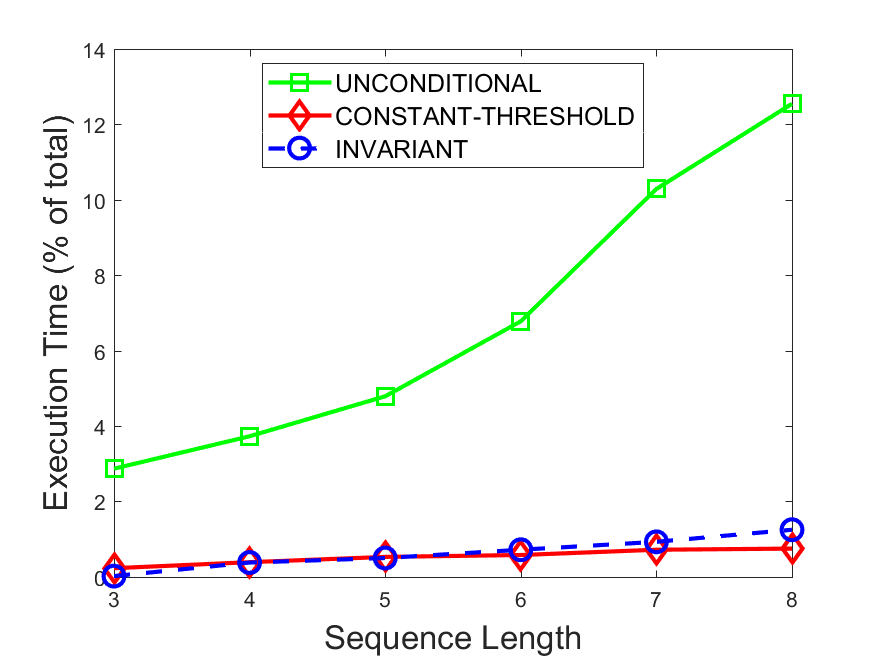
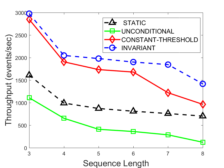
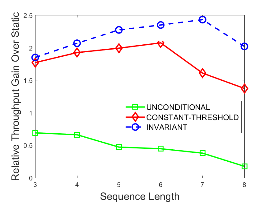
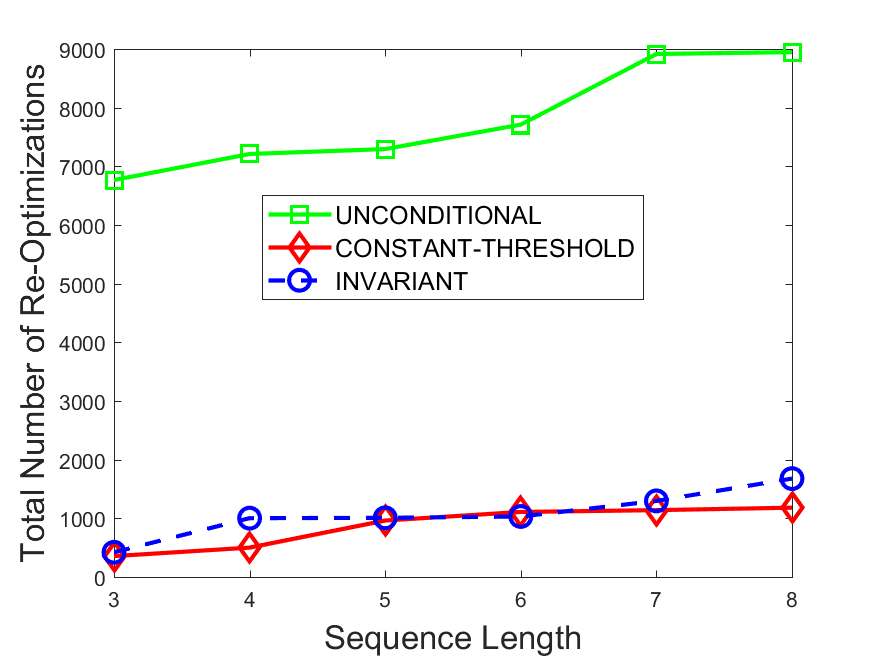
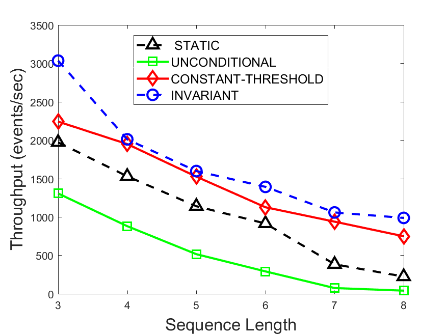
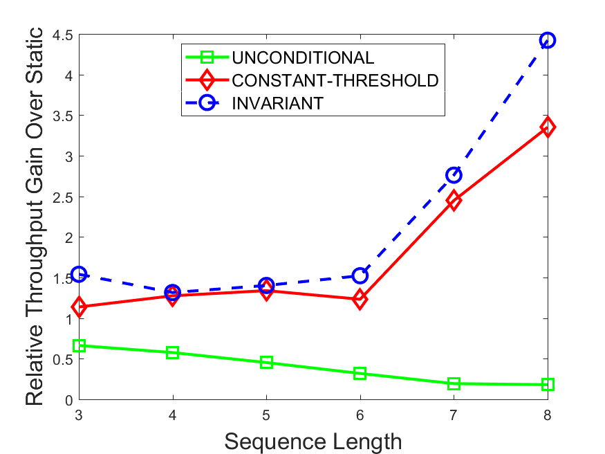
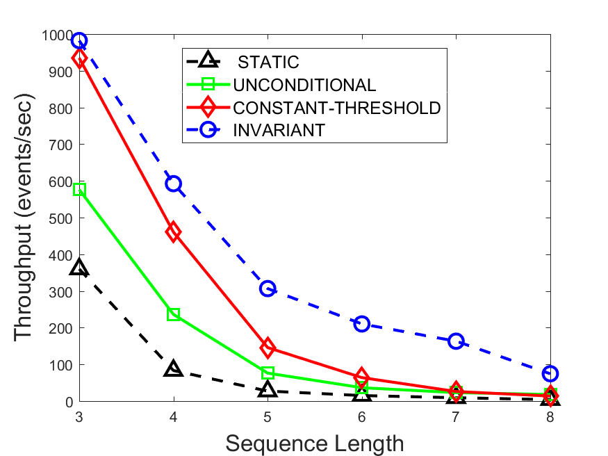
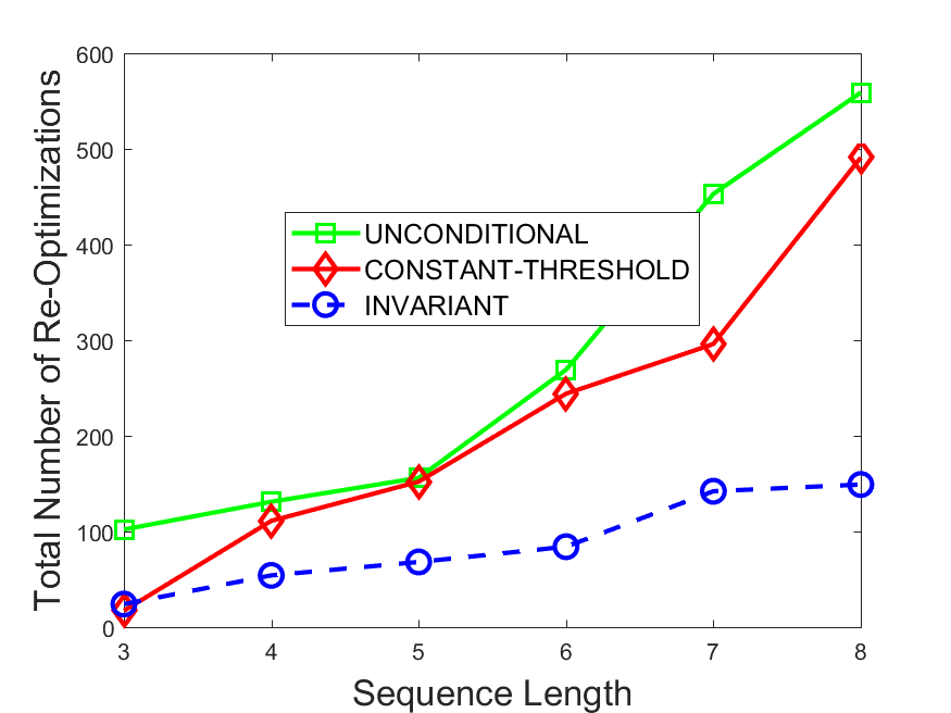
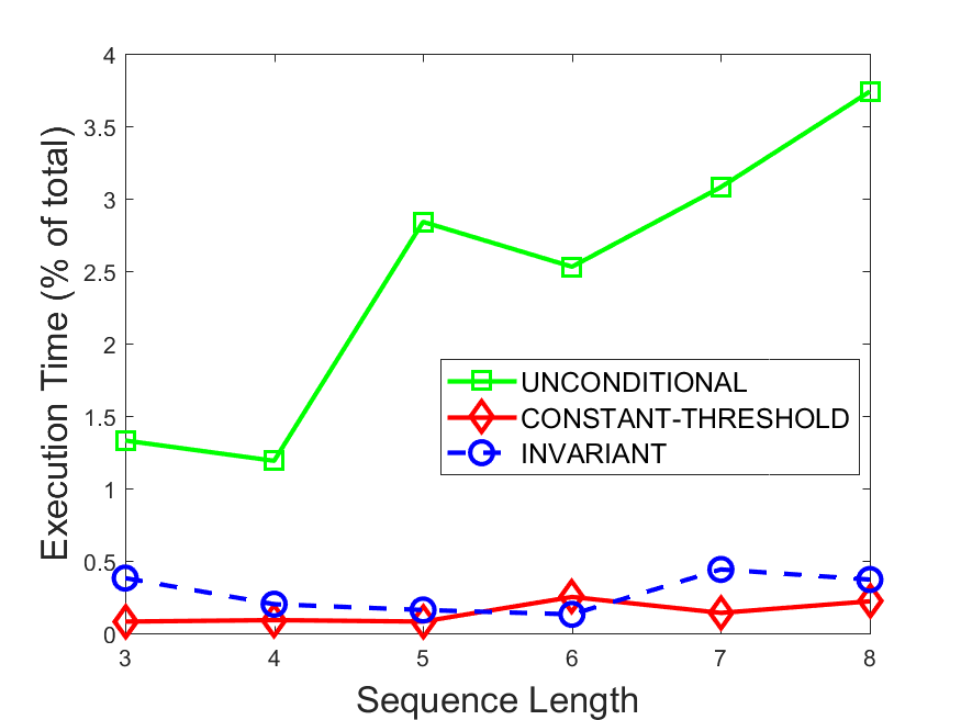
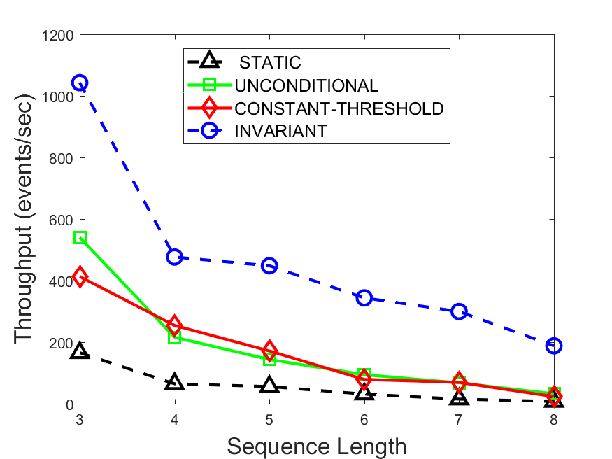
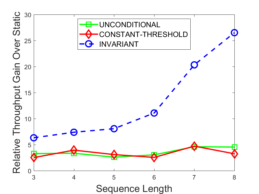
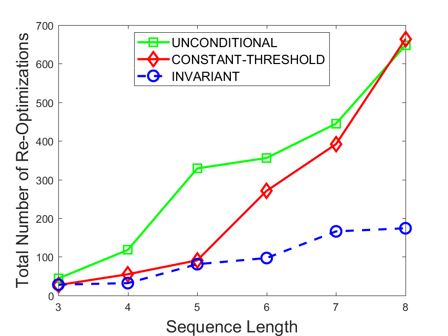
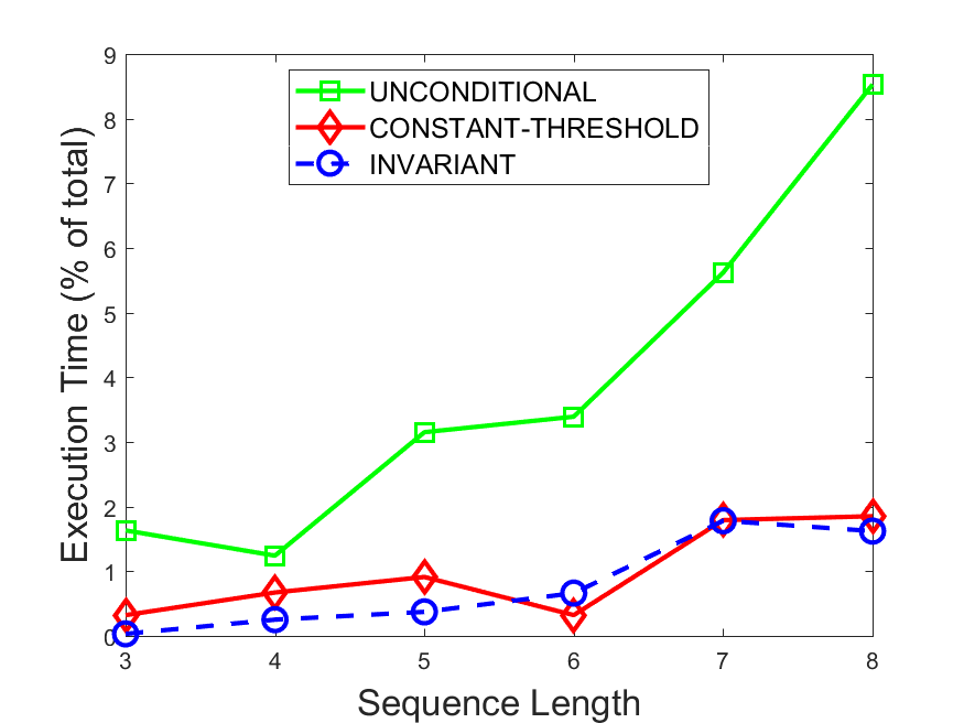
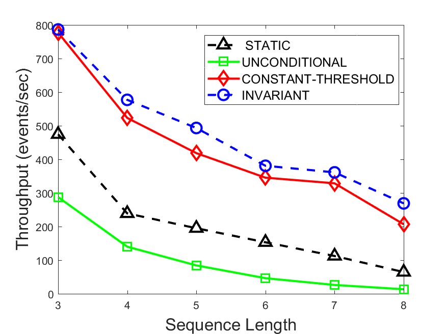
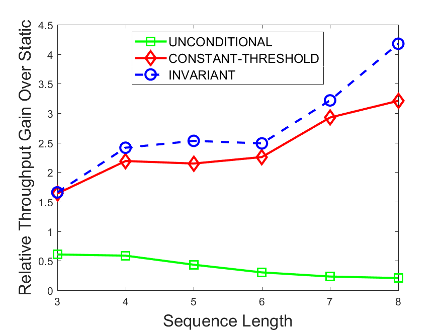
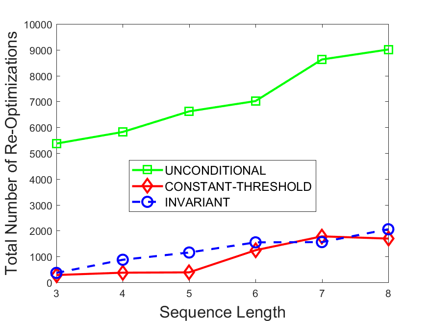
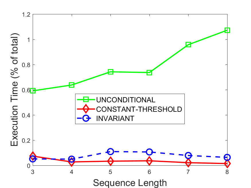
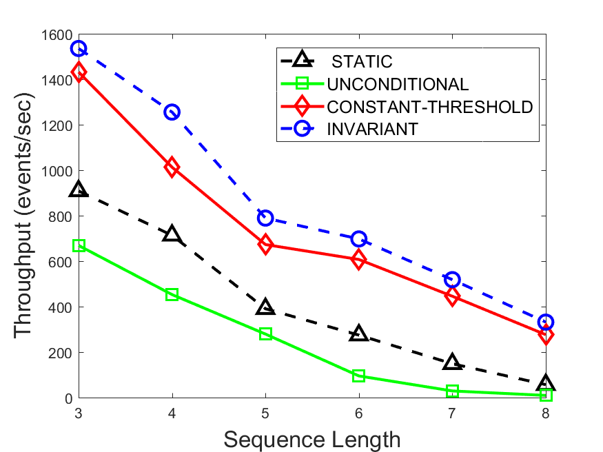
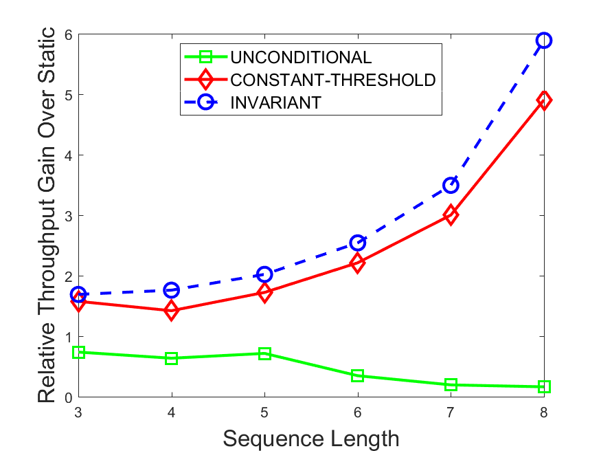
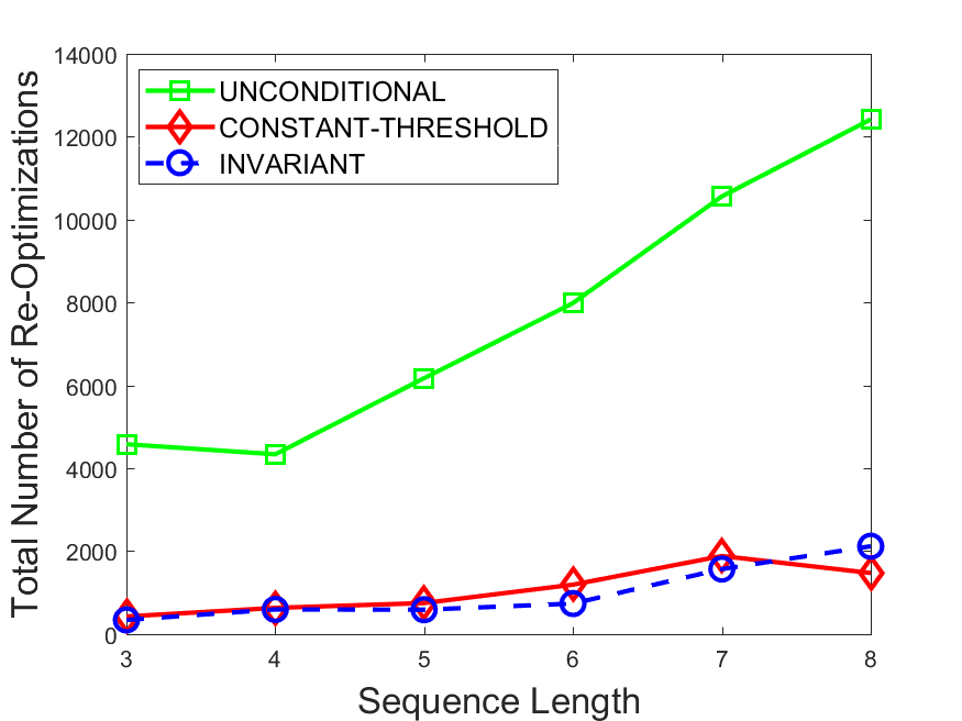
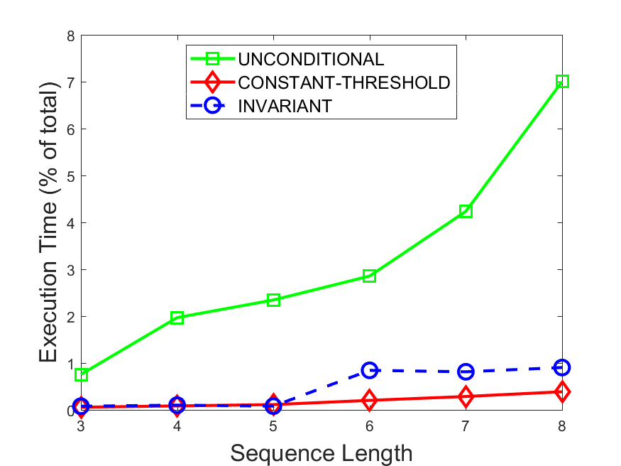
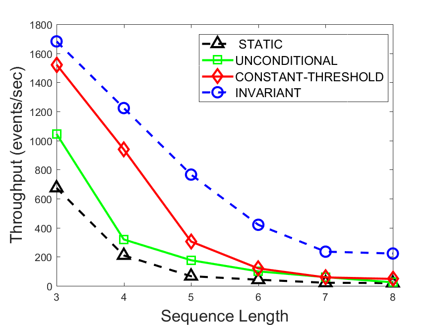
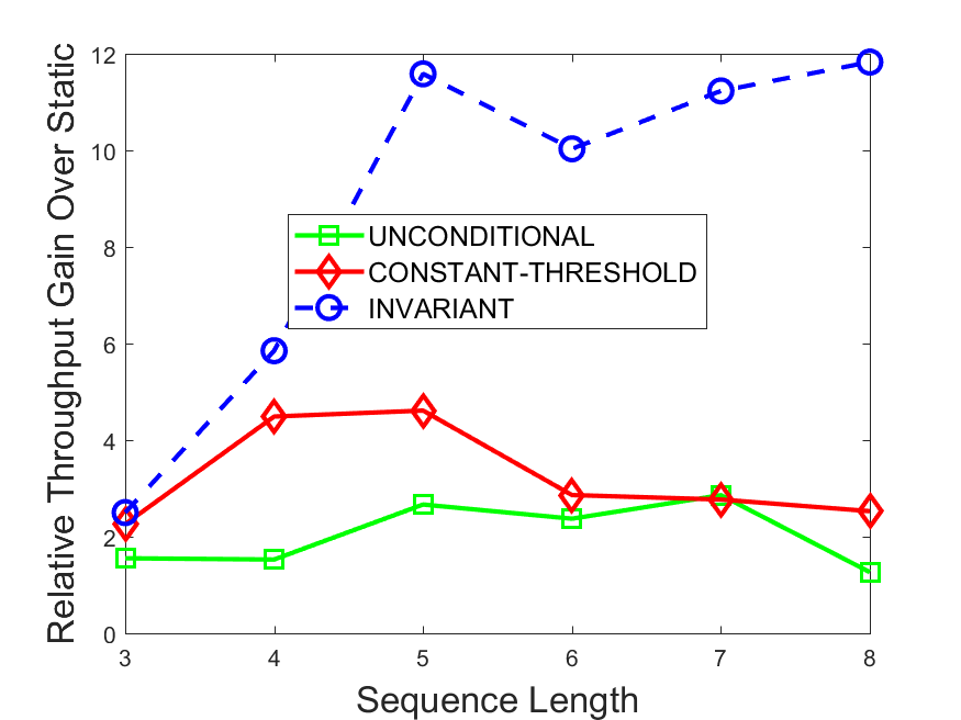
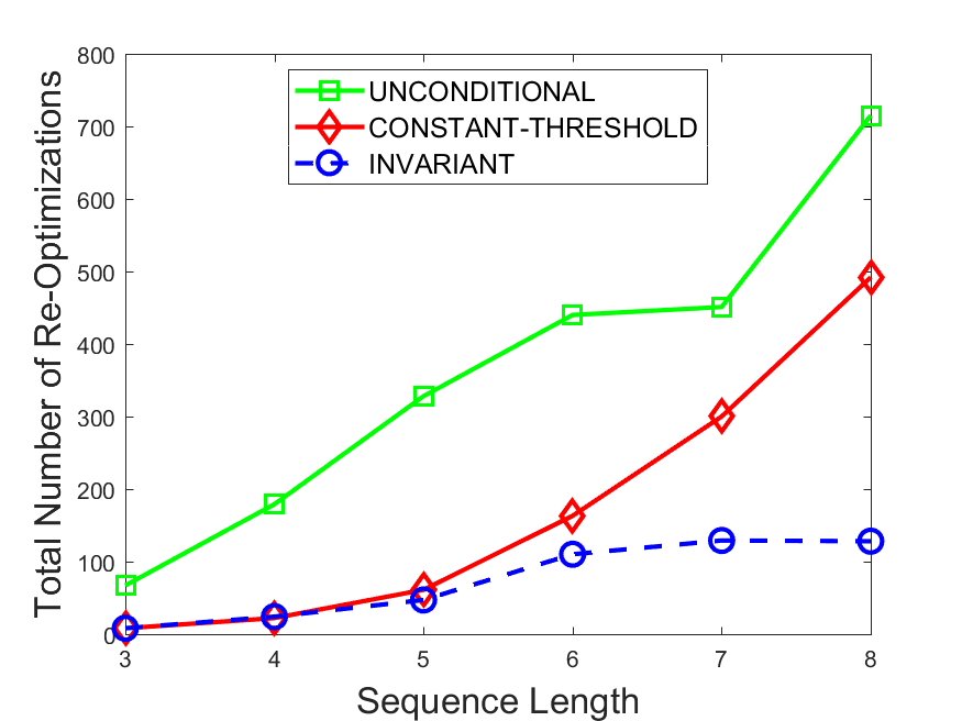
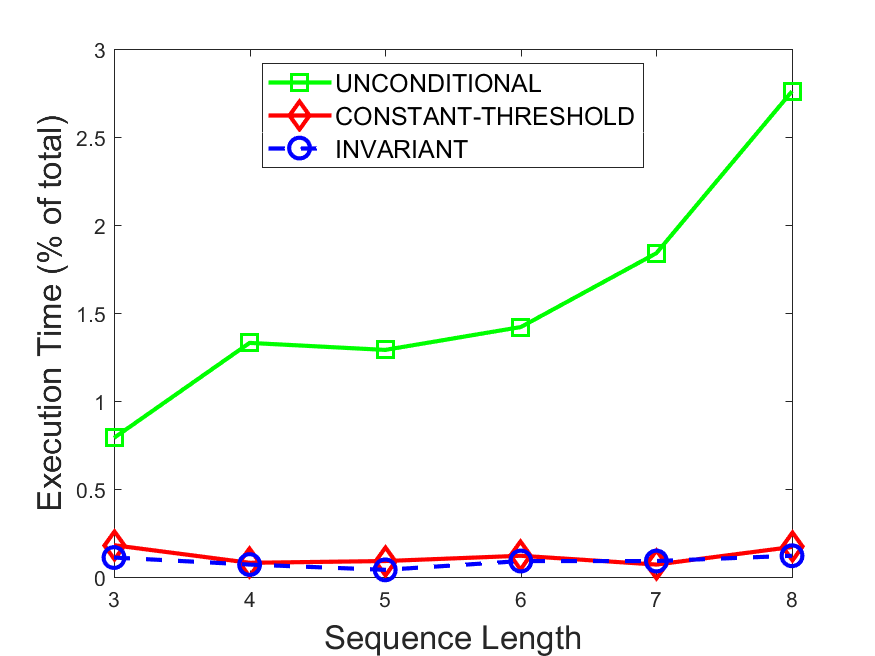
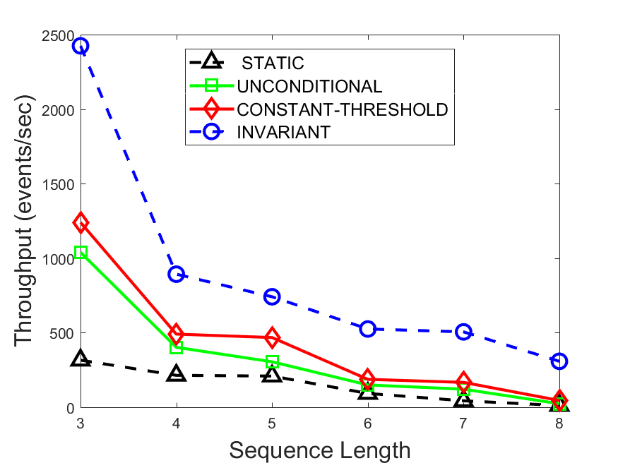
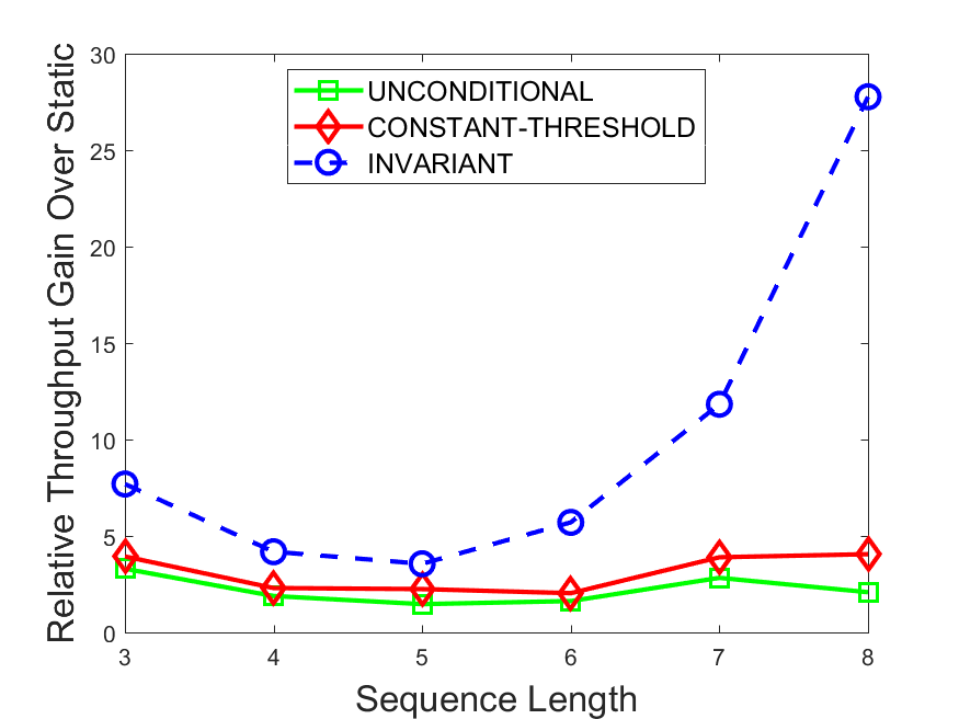
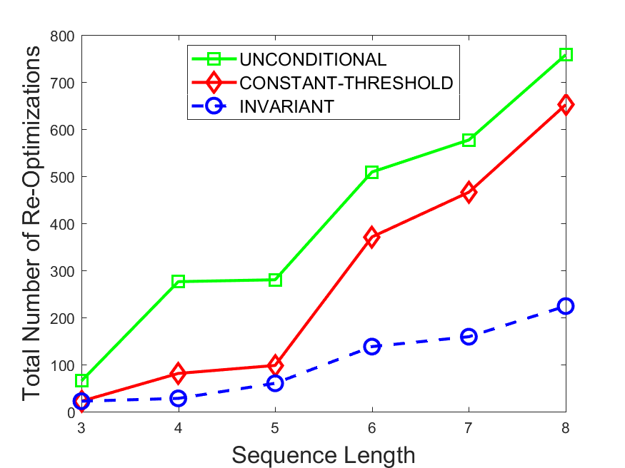
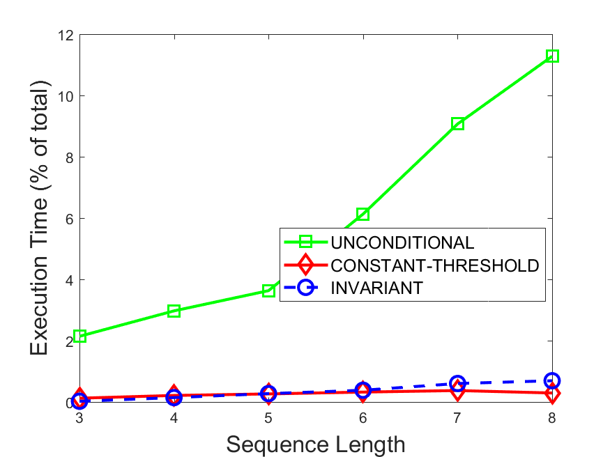
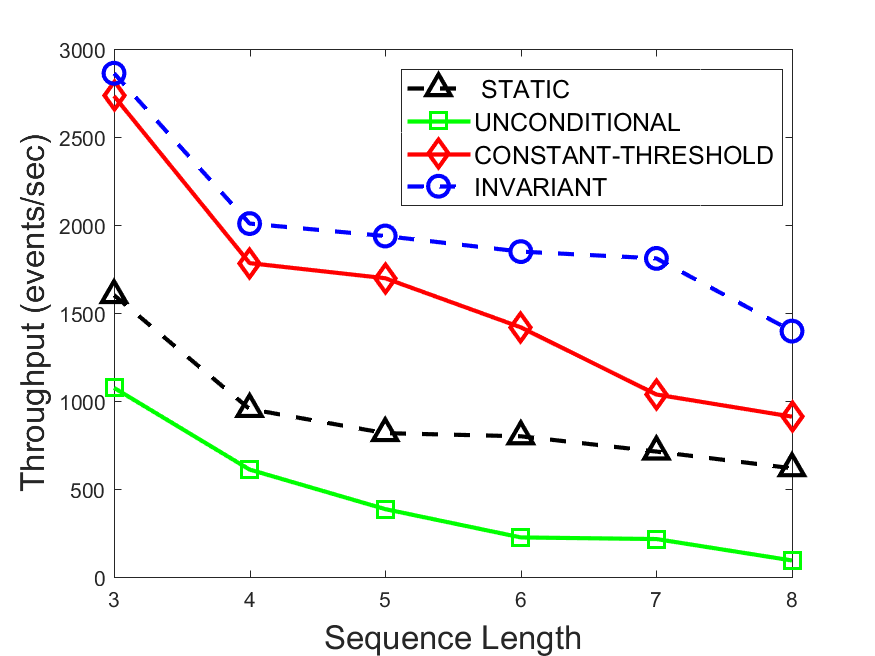
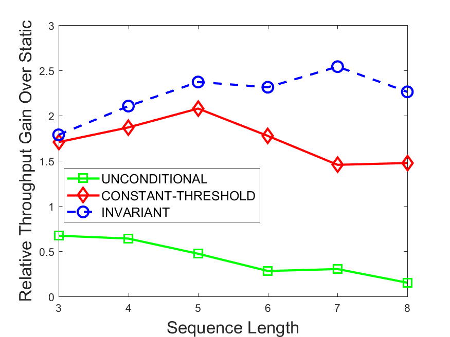
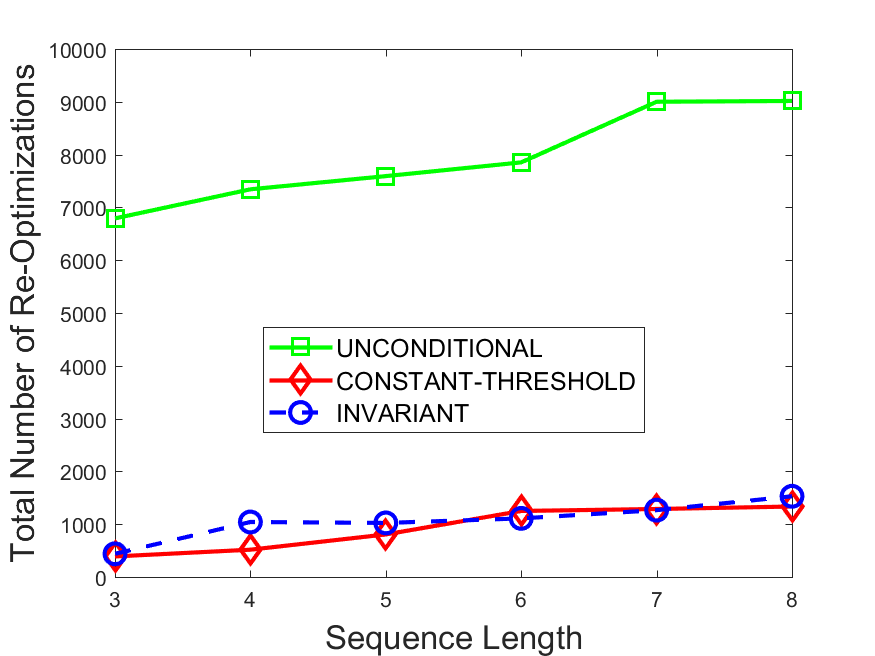
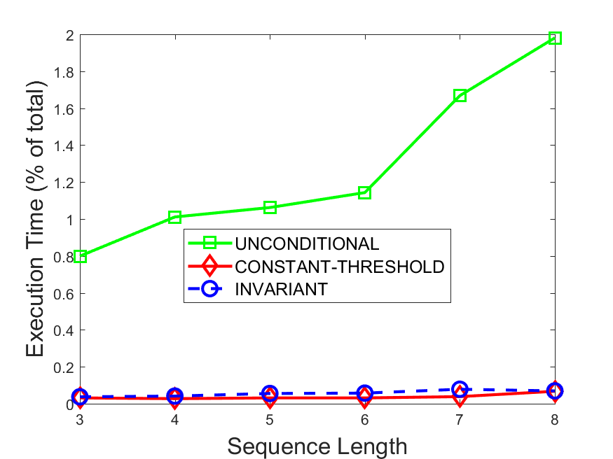
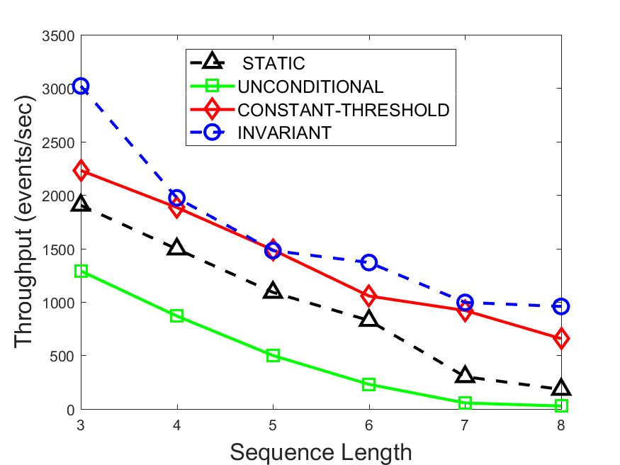
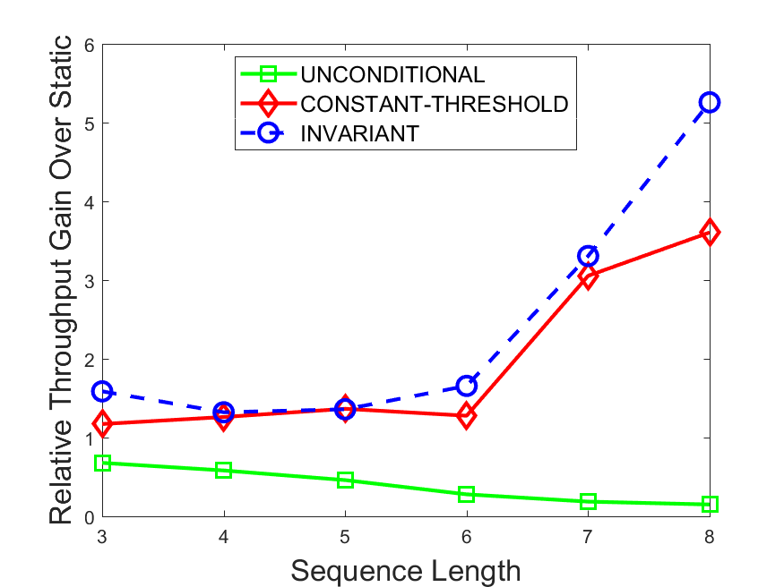
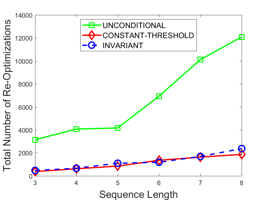
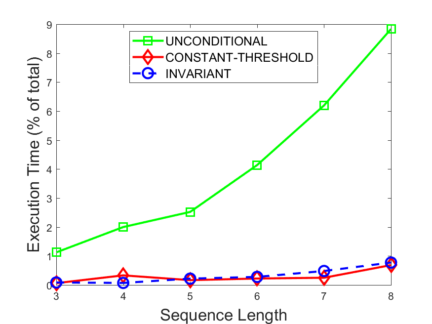
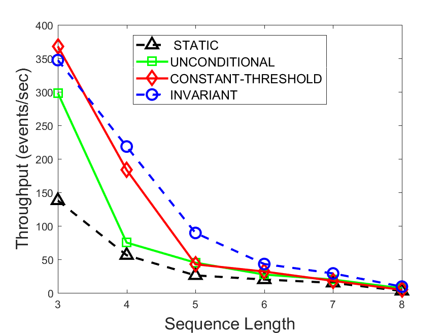
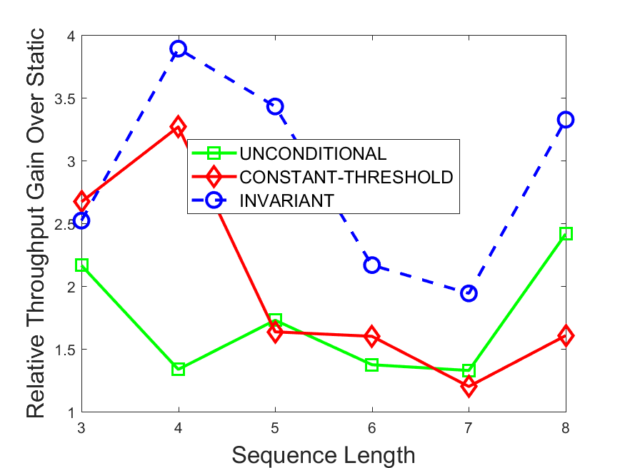
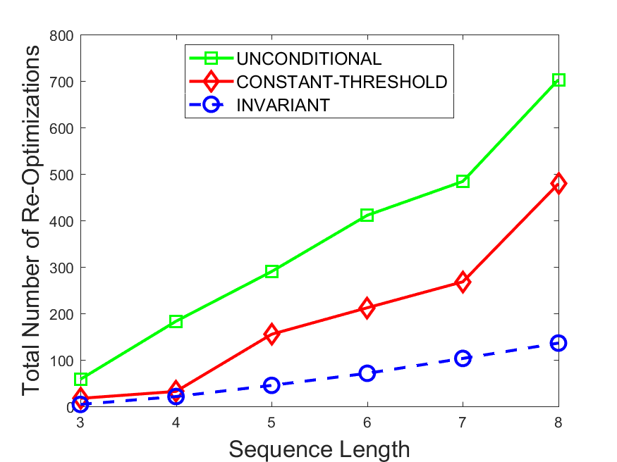
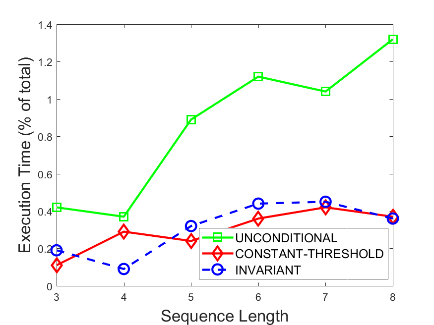
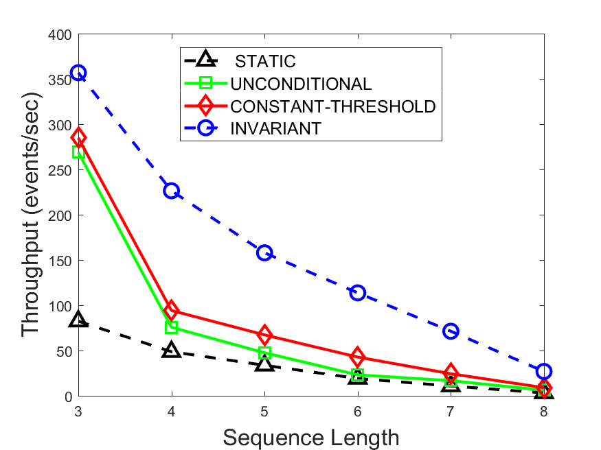
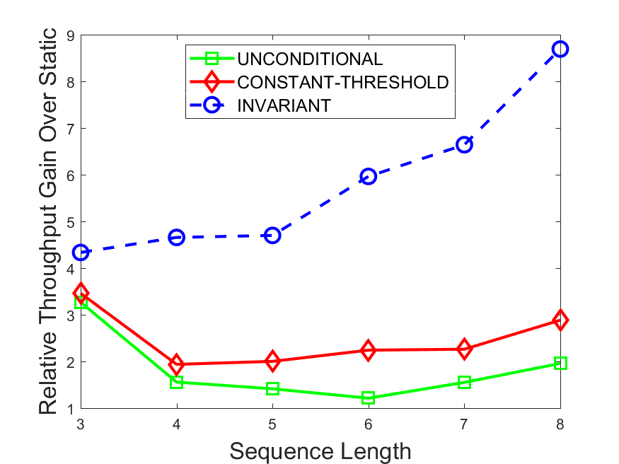
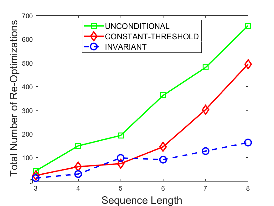
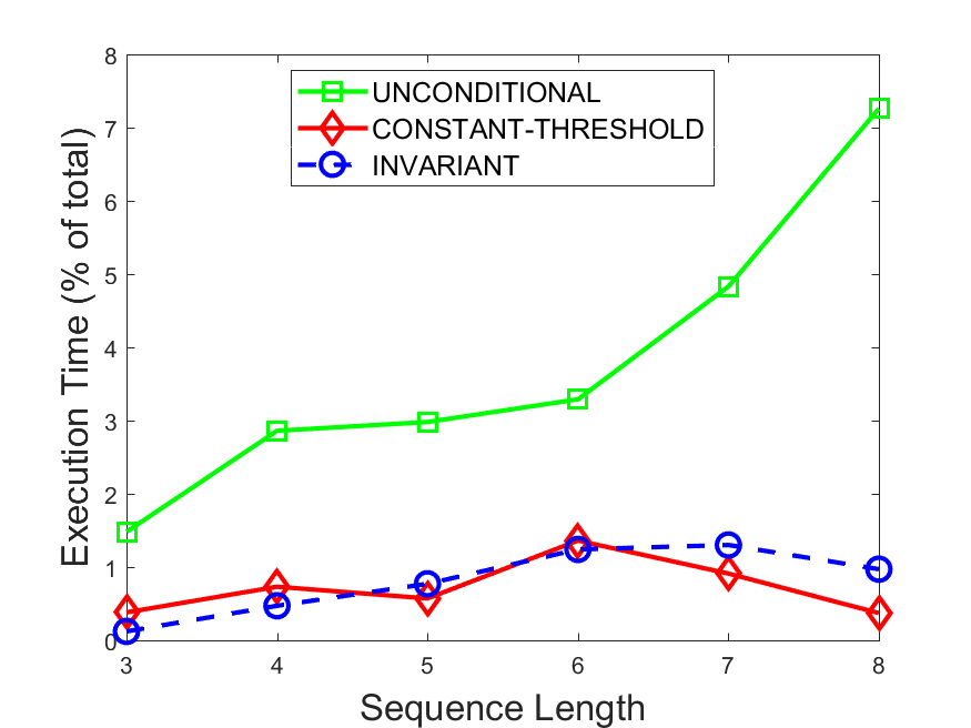
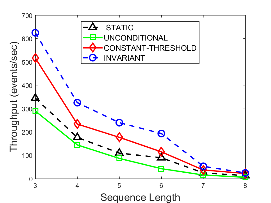
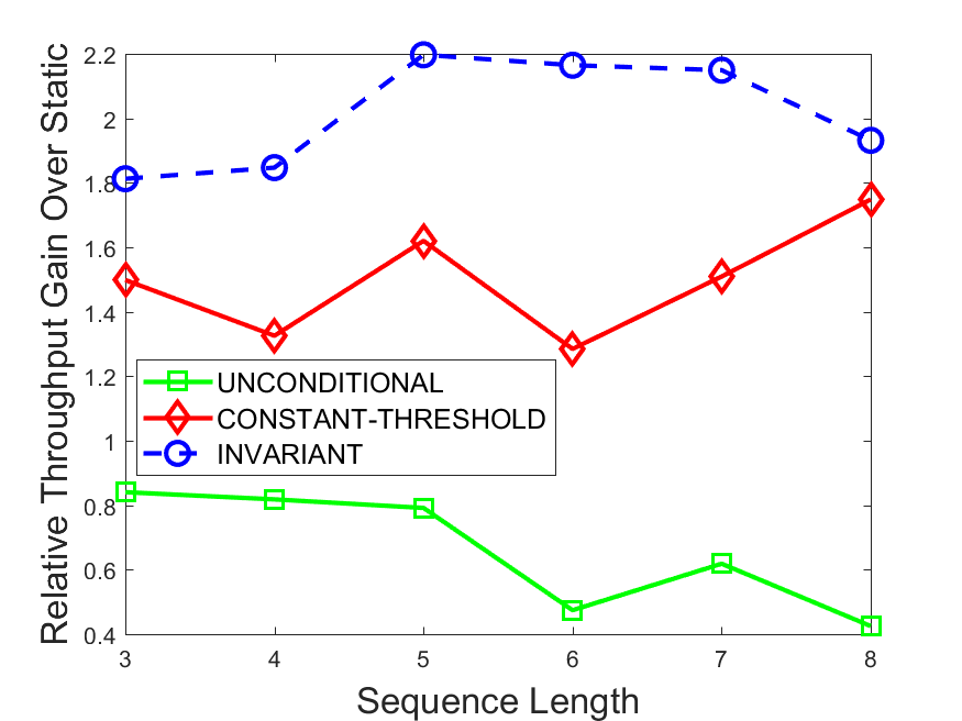
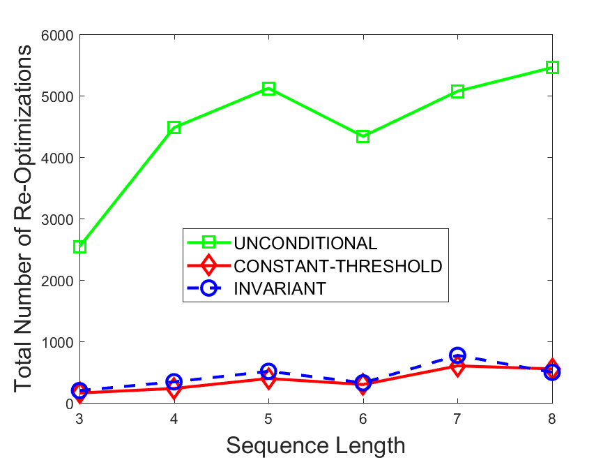
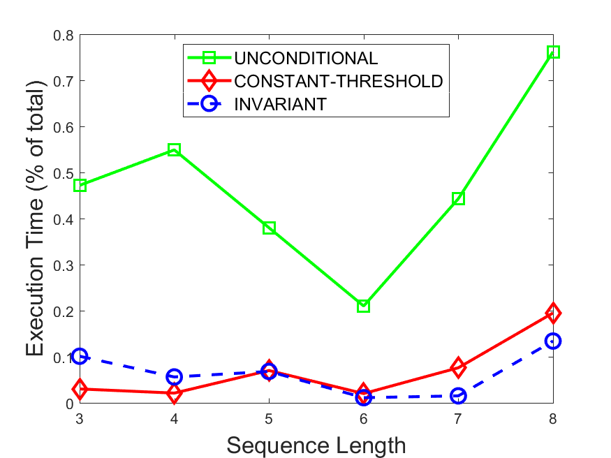
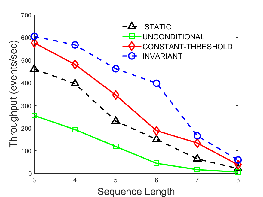
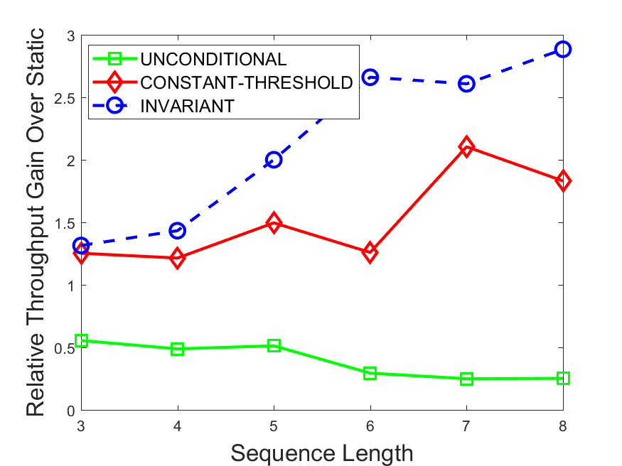
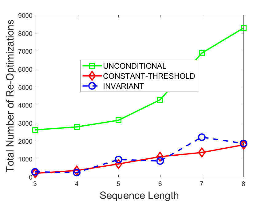
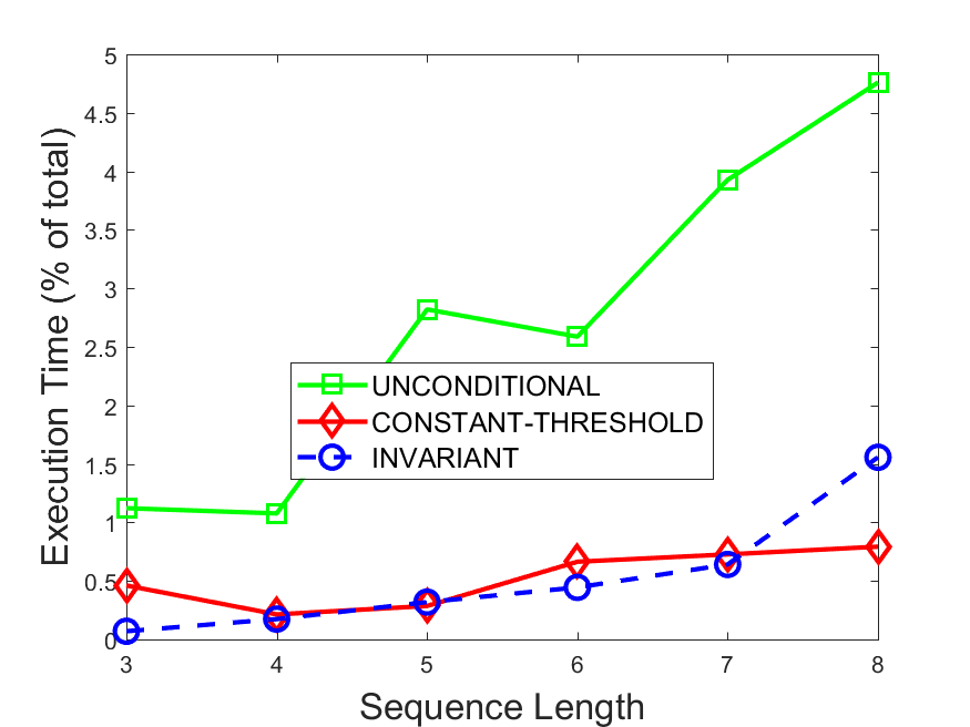
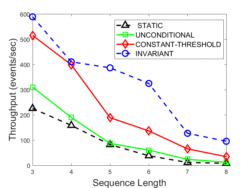
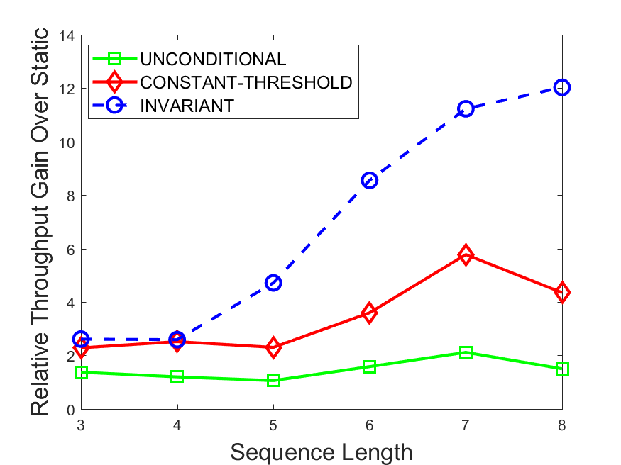
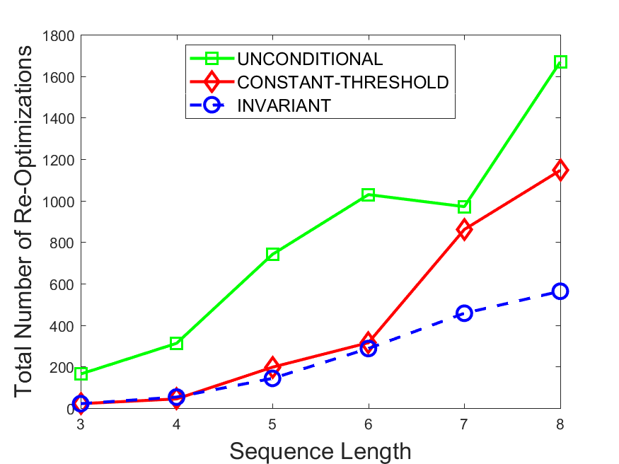
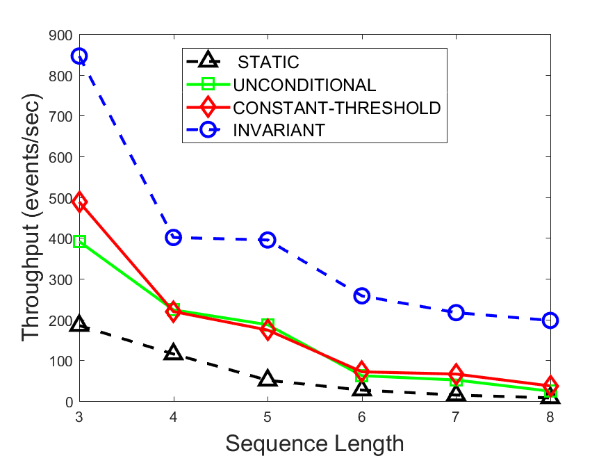
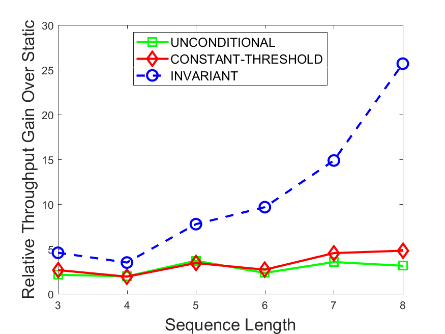
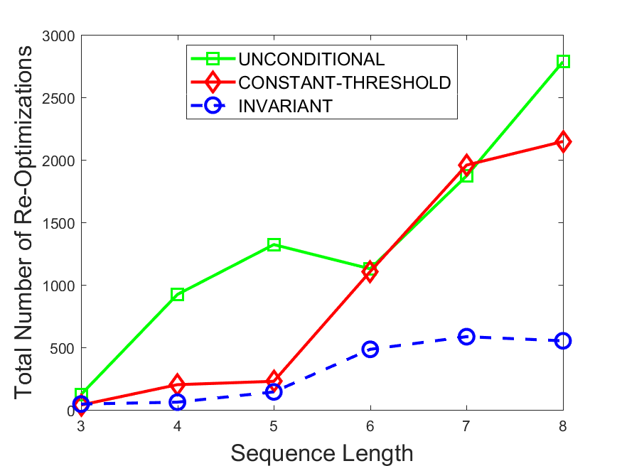
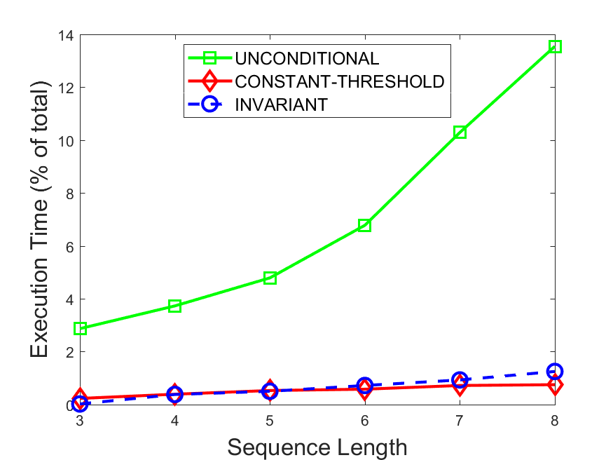
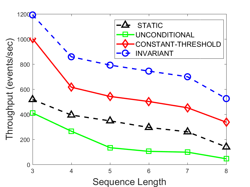
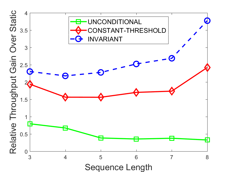
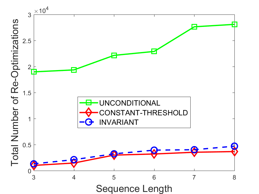
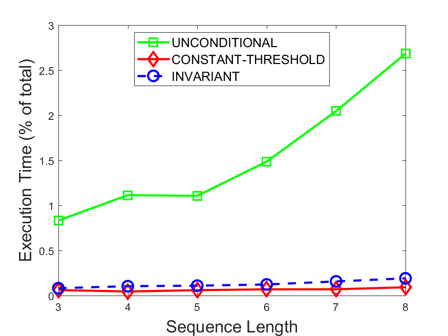
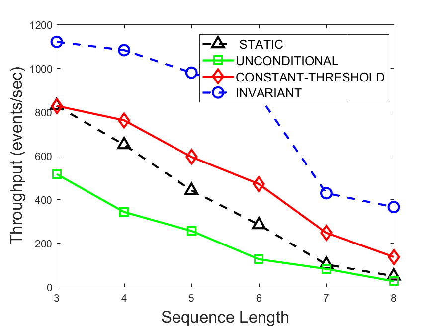
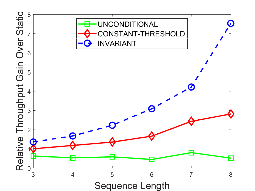
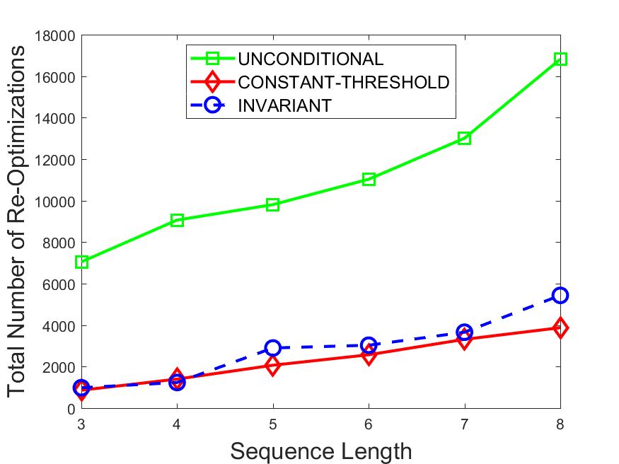
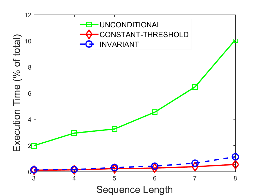
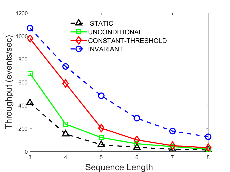
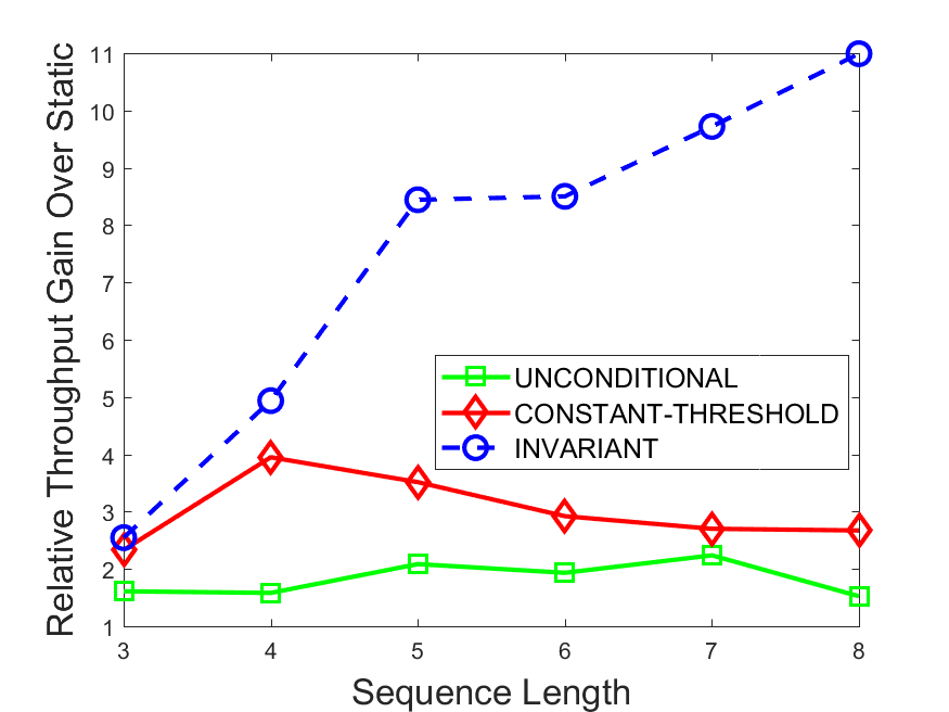
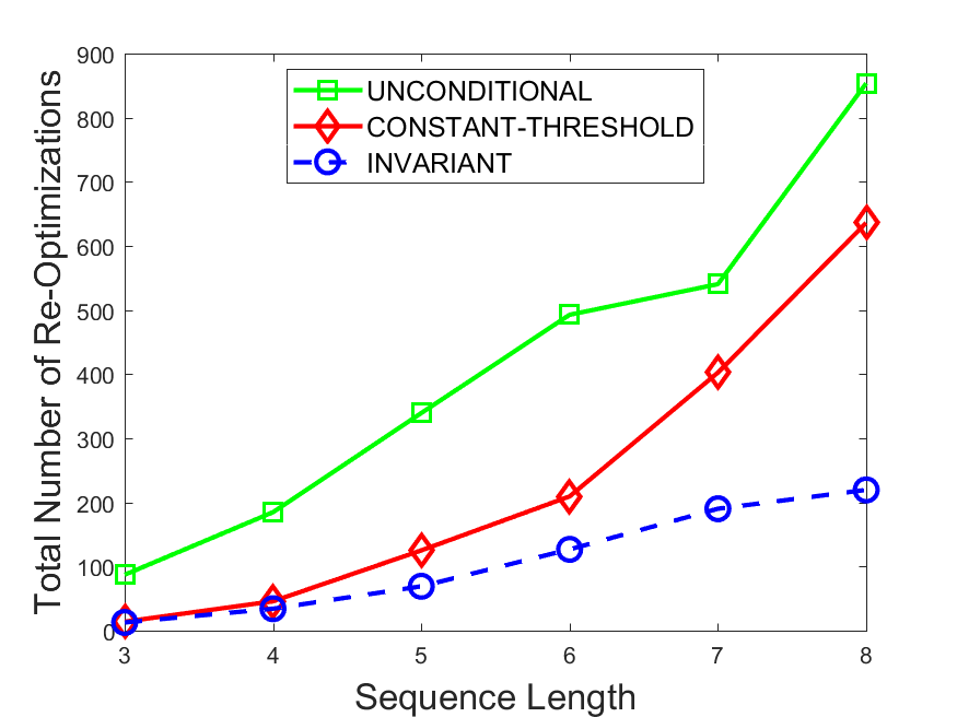
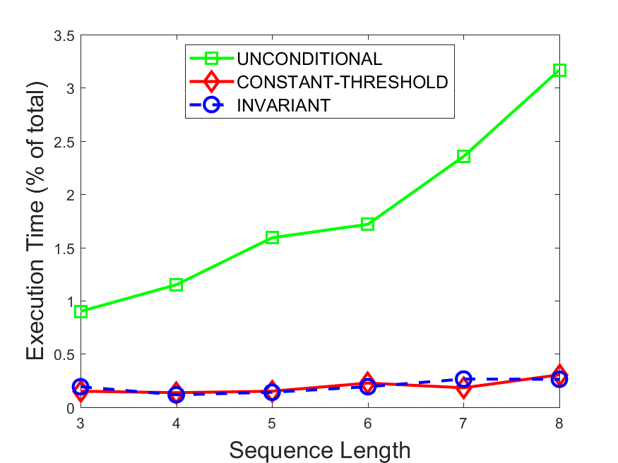
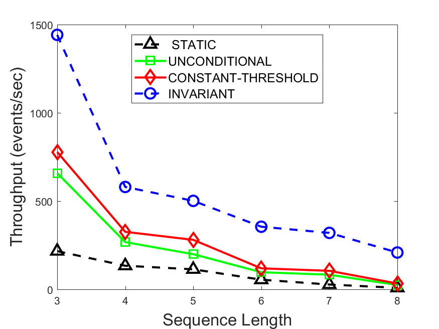
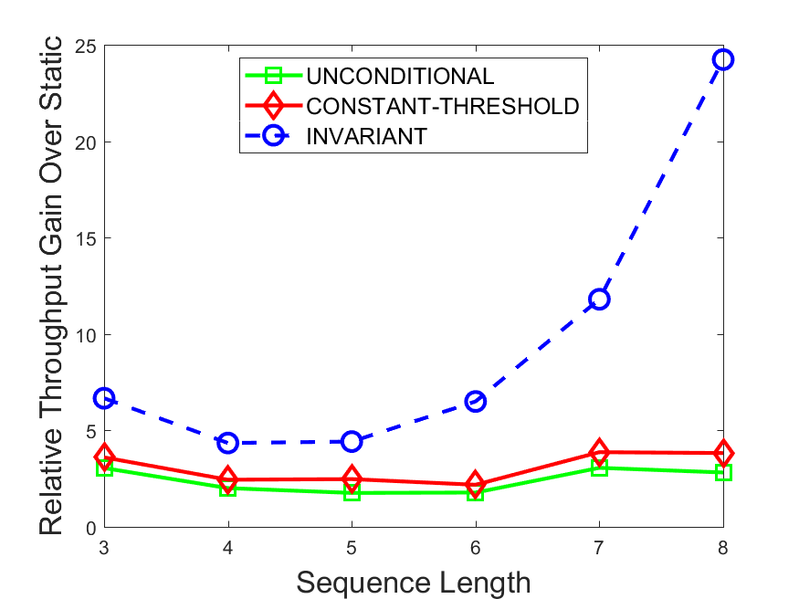
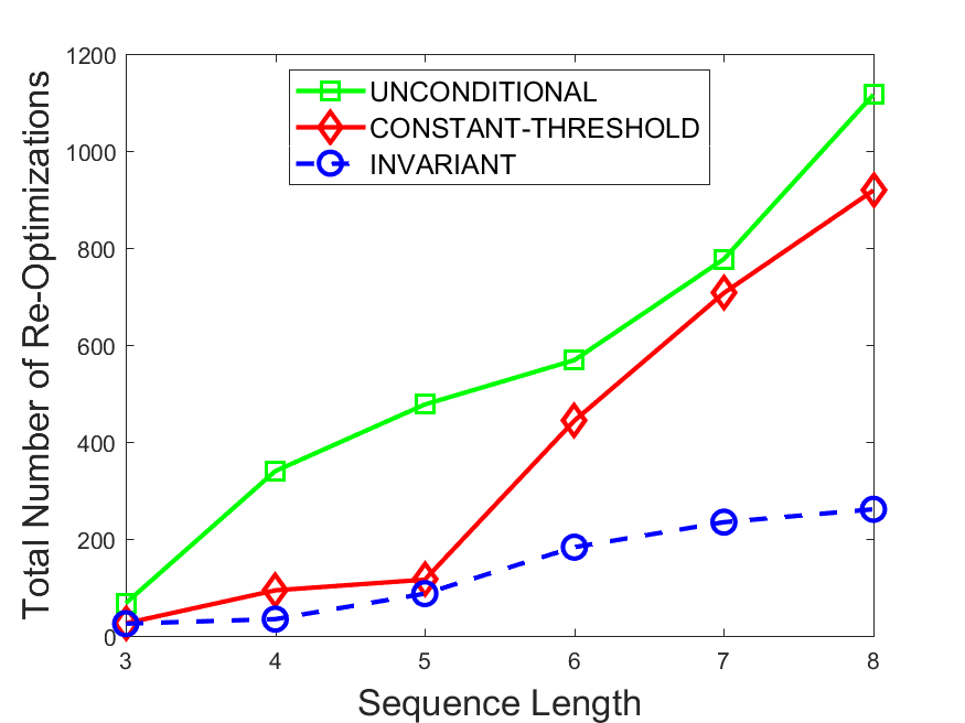
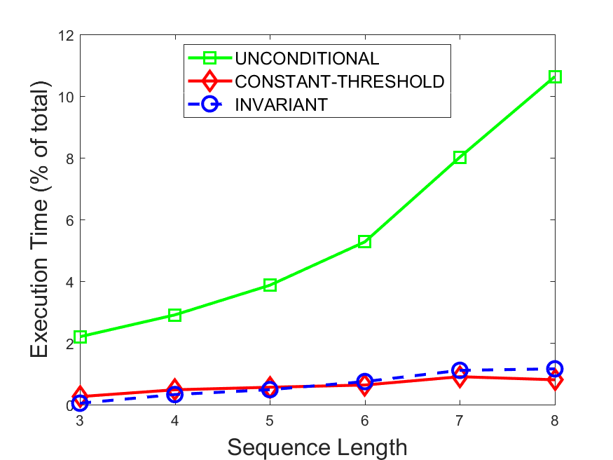
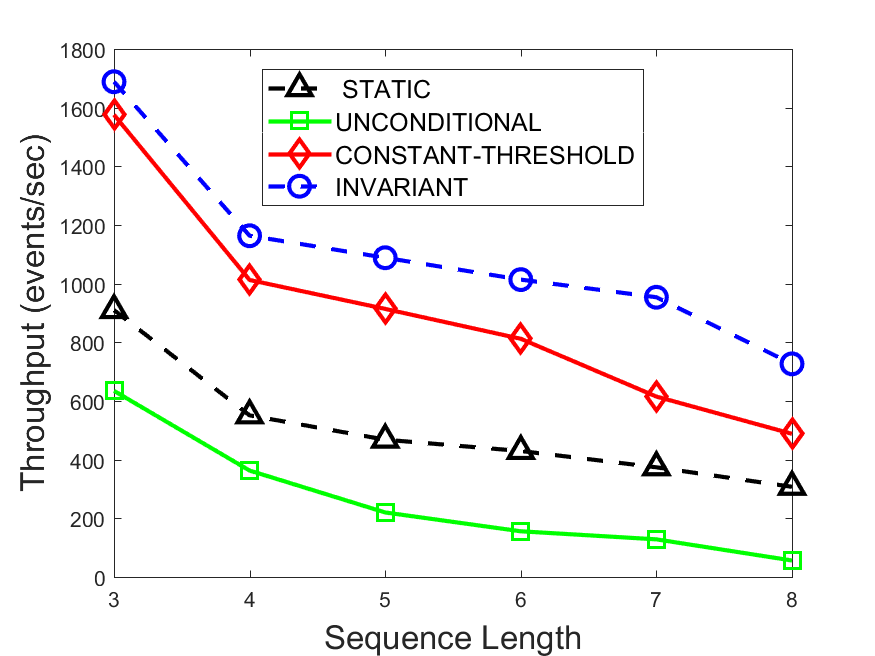
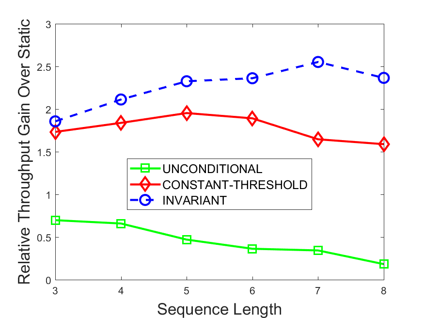
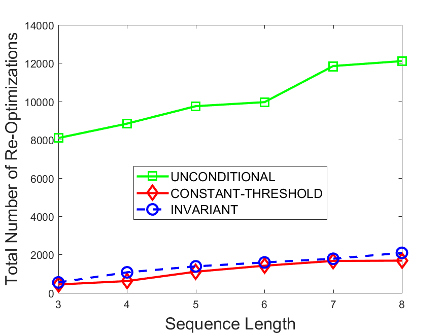
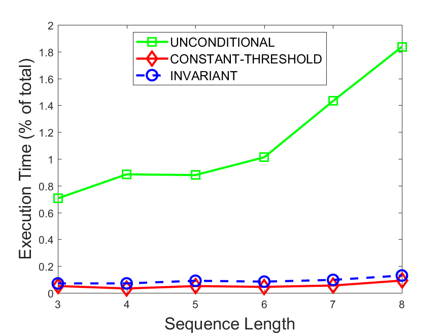
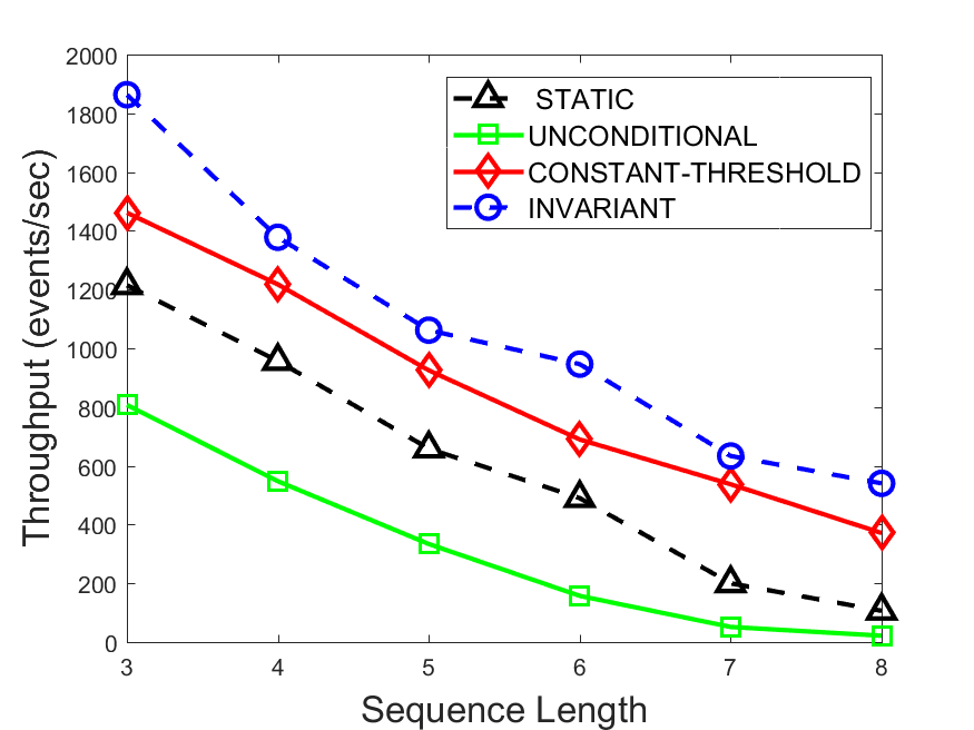
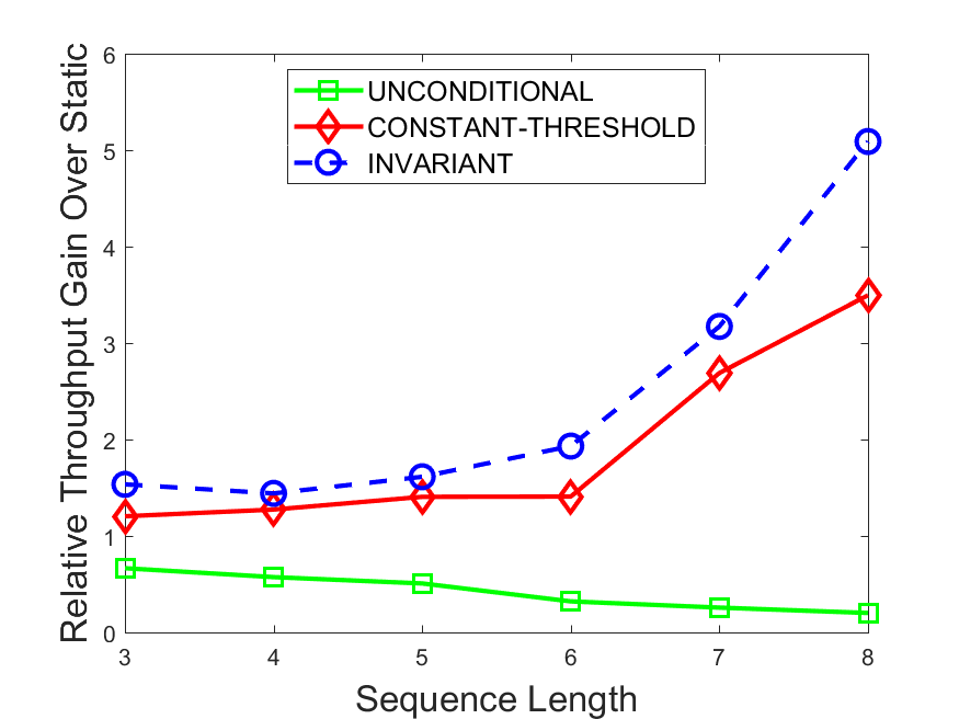
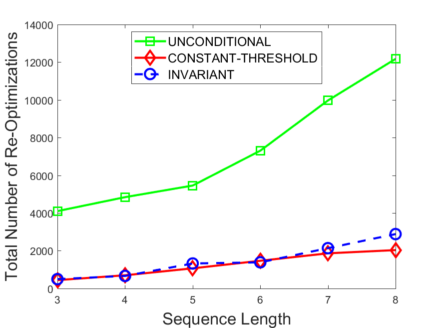
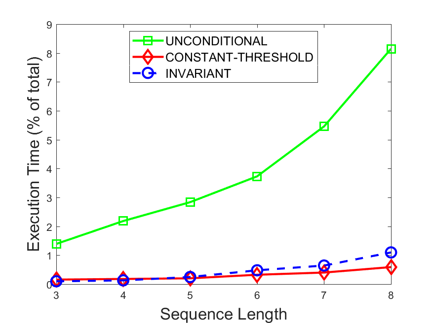
Figures 6-9 summarize the results. Each figure represents the measurements for a particular dataset-algorithm combination and contains four graphs, presenting different statistics as a function of the pattern size. The first graph presents the throughput achieved using each of the adaptation methods. Here, we have also included the “static” method in our study, where no adaptation is supported and the dataset is processed using a single, predefined plan. The second graph is a different way of viewing the previous one, comparing the adaptation methods by the relative speedup they achieve over the “static plan” approach. The third graph depicts the total number of reoptimizations (actual plan replacements) recorded during each run. Finally, we report the computational overhead of each method, that is, a percentage of the total execution time spent on executions of and (i.e., checking whether a reoptimization is necessary and computing new plans).
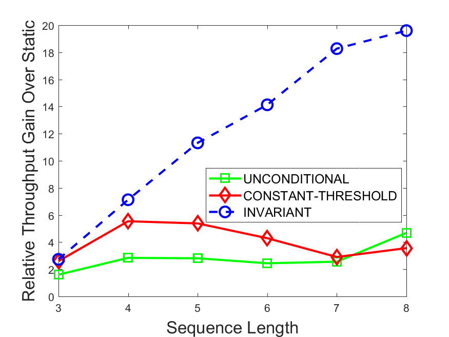
The throughput comparison demonstrates the superiority of the invariant-based method over its alternatives for all scenarios. Its biggest performance gain is achieved in the traffic scenario, characterized by high skew and major statistic shifts (Figures 6-7). This gain reaches its peak for larger patterns, with the maximal recorded performance of more than 6 times that of the second-best constant-threshold method: the greater the discrepancy between the data characteristics, the more difficult it is to find a single threshold to accurately monitor all the changes. Since this discrepancy may only increase as more statistic values are added to the monitored set, we expect the superiority of this method to keep growing with the pattern size beyond the values we experimented with. Figures 6LABEL:sub@fig:relative-throughput-7LABEL:sub@fig:relative-throughput provide a clear illustration of the above phenomenon and of the invariant-based method scalability. Note also that, for larger pattern sizes, the constant-threshold method nearly converges to the unconditional one due to the increasing number of false positives it produces.
For the stocks dataset (Figures 8-9), the throughput measurements for the constant-threshold and the invariant-based methods are considerably closer. Due to the near-uniformity of the statistic values and of their variances, finding a single is sufficient to recognize most important changes. Hence, the precision of the constant-threshold method is very high on this input. Nevertheless, the invariant-based method achieves a performance speedup for this dataset as well (albeit only about 30-60%) without adding significant overhead. Also, for the same reason, the static plan performs reasonably well in this scenario, decidedly outperforming the unconditional method. The latter suffers from extreme over-adapting to the numerous small-scale statistic shifts.
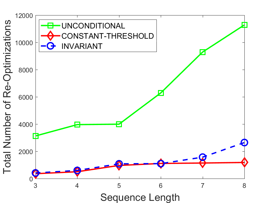
The total number of reoptimizations performed in each scenario (Figures 6LABEL:sub@fig:plan-switch-9LABEL:sub@fig:plan-switch) backs up and augments the above results. The invariant-based method consistently requires few plan replacements while also achieving the best throughput. The extremely high numbers produced by the unconditional strategy lead to its poor performance. For the traffic dataset, the constant-threshold method tends to approach these numbers for larger patterns. This can either be a sign of multiple false positives or over-adapting. For the stocks dataset, this method becomes more similar to the invariant-based one, executing nearly identical reoptimizations.
Figures 6LABEL:sub@fig:overhead-9LABEL:sub@fig:overhead present the computational overhead of the compared approaches. Here, the same behavior is observed for all dataset-algorithm combinations. While the invariant-based and the constant-threshold methods consume negligible system resources, unconditional reoptimization results in up to 11% of the running time devoted to the adaptation process.
As evident by the experiments with stock market data (Figures 8-9), smaller number of reoptimizations and lower computational overhead do not necessarily result in better overall system performance. On this dataset, the invariant-based method achieves the highest throughput despite a slightly higher overhead as compared to the second-best constant-threshold method. This can be attributed to the false negatives of the latter, that is, cases in which it missed a reoptimization opportunity and kept using an old plan despite a better one being available.
In all experiments, the gains of the invariant-based method were considerably higher for ZStream algorithm than for the greedy one. There are two reasons for this result. First, the more complex structure of the tree-based plans makes it more difficult to capture the dependencies between plan components without fine-grained invariants. Second, as this algorithm is more computationally expensive, the penalty for a redundant reoptimization is higher. Following these observations, we believe that the invariant-based method is capable of achieving even larger benefit for more advanced and precise (and hence more complex) plan generation algorithms. Utilizing this method will thus encourage the adoption of such algorithms by CEP engines.
6 Related Work
Complex event processing is an increasingly active research field [26]. The origins of CEP systems can be traced to older data stream managements systems (DSMSs), including Aurora/Borealis [4], Stream [12], TelegraphCQ [21], and NiagaraCQ [22]. This was followed by the emergence of a broad variety of solutions for detecting occurrences of situations of interest, as opposed to generic data, including frameworks such as SASE/SASE+ [49, 7, 51], CEDR [18], Cayuga [28], T-Rex [25] and Amit [6]. Esper [2] and IBM System S [11] are examples of widely used commercial CEP providers.
Many CEP approaches incorporate NFAs as their primary evaluation structure [49, 28, 25]. Various extensions to this model were developed, such as AFA [20] and lazy NFA [36]. ZStream [42] utilizes tree-based detection plans for the representation of event patterns. Event processing networks [30] is another conceptual model, presenting a pattern as a network of simple agents.
Multiple works have addressed the broad range of CEP optimization opportunities arising when the statistical characteristics of the primitive events are taken into account. In [8] “plan-based evaluation” is described, where the arrival rates of events are exploited to reduce network communication costs. The authors of NextCEP [45] propose a framework for pattern rewriting in which operator properties are utilized to assign a cost to every candidate evaluation plan. Then, a search algorithm (either greedy or dynamic) is applied to select the lowest cost detection scheme. ZStream [42] applies a set of algebraic rule-based transformations on a given pattern, and then reorders the operators to minimize the cost of a plan.
Adaptive query processing (AQP) is the widely studied problem of adapting a query plan to the unstable data characteristics [29]. Multiple solutions consider traditional data-bases [5, 32, 15, 41, 33, 46]. The mid-query reoptimization mechanism [33], one of the first to possess adaptive properties, collects statistics at the predefined checkpoints and compares them to the past estimates. If severe deviation is observed, the remainder of the data is processed using a new plan. The methods described in [15] and [41] are the closest in spirit to our work. Rather than executing reoptimization on a periodic basis or upon a constant change, the authors compute an individual range for each monitored value within which the current plan is considered close-to-optimal.
The field of stream processing has developed adaptive techniques of its own. A-Greedy [16] is an algorithm for adaptive ordering of pipelined filters, providing strong theoretical guarantees. Similarly to our method, it detects violations of invariants defined on the filter drop probabilities. The authors of [39] describe “incremental reoptimization,” where the optimizer constantly attempts to locate a better plan using efficient search and pruning techniques. Eddy [13, 19, 40] presents stateless routing operators, redirecting incoming tuples to query operators according to a predefined routing policy. This system discovers execution routes on-the-fly in a per-tuple manner. Query Mesh [43] is a middle-ground approach, maintaining a set of plans and using a classifier to select a plan for each data item. Large DSMSs have also incorporated adaptive mechanisms [48, 17].
The majority of the proposed CEP techniques are deprived from adaptivity considerations [31]. The two notable exceptions, ZStream [42] and tree-based NFA [36] were covered in detail above. Additional works labeled as ’adaptive’ refer to on-the-fly switching between several detection algorithms [44, 50] or dynamic rule mining [23, 38].
7 Conclusions and Future Work
In this paper, we discussed the problem of efficient adaptation of a CEP system to on-the-fly changes in the statistical properties of the data. A new method was presented to avoid redundant reoptimizations of the pattern evaluation plan by periodically verifying a small set of simple conditions defined on the monitored data characteristics, such as the arrival rates and the predicate selectivities. We proved that validating this set of conditions will only fail if a better evaluation plan is available. We applied our method on two real-life algorithms for plan generation and experimentally demonstrated the achieved performance gain.
In addition to the research of distance estimators (Section 3.4), one area of interest that was not yet addressed by the existing approaches is the multi-pattern adaptive CEP, where the system is given a set of patterns possibly containing common subexpressions. In this case, the detection process typically follows a single global plan that exploits sharing opportunities, rather than executing multiple individual plans in parallel. While our method can be trivially applied to multi-pattern systems with no sharing, substantially more sophisticated optimization techniques are required for the general case. We intend to target this research direction in our future work.
References
- [1] http://www.eoddata.com.
- [2] http://www.espertech.com.
- [3] E. Aarts and J. Lenstra, editors. Local Search in Combinatorial Optimization. John Wiley & Sons, Inc., New York, NY, USA, 1st edition, 1997.
- [4] D. J. Abadi, Y. Ahmad, M. Balazinska, M. Cherniack, J. Hwang, W. Lindner, A. S. Maskey, E. Rasin, E. Ryvkina, N. Tatbul, Y. Xing, and S. Zdonik. The design of the borealis stream processing engine. In CIDR, pages 277–289, 2005.
- [5] M. Acosta, M. Vidal, T. Lampo, J. Castillo, and E. Ruckhaus. Anapsid: An adaptive query processing engine for sparql endpoints. In International Semantic Web Conference (1), volume 7031, pages 18–34. Springer, 2011.
- [6] A. Adi and O. Etzion. Amit - the situation manager. The VLDB Journal, 13(2):177–203, 2004.
- [7] J. Agrawal, Y. Diao, D. Gyllstrom, and N. Immerman. Efficient pattern matching over event streams. In SIGMOD, pages 147–160, 2006.
- [8] M. Akdere, U. Çetintemel, and N. Tatbul. Plan-based complex event detection across distributed sources. Proc. VLDB Endow., 1(1):66–77, 2008.
- [9] M. Ali, F. Gao, and A. Mileo. Citybench: A configurable benchmark to evaluate rsp engines using smart city datasets. In Proceedings of ISWC 2015 - 14th International Semantic Web Conference, pages 374–389, Bethlehem, PA, USA, 2015. W3C.
- [10] A. Aly, W. Aref, M. Ouzzani, and H. Mahmoud. JISC: adaptive stream processing using just-in-time state completion. In Proceedings of the 17th International Conference on Extending Database Technology, Athens, Greece, March 24-28, 2014., pages 73–84.
- [11] L. Amini, H. Andrade, R. Bhagwan, F. Eskesen, R. King, P. Selo, Y. Park, and C. Venkatramani. Spc: A distributed, scalable platform for data mining. In Proceedings of the 4th International Workshop on Data Mining Standards, Services and Platforms, pages 27–37, New York, NY, USA, 2006. ACM.
- [12] A. Arasu, B. Babcock, S. Babu, J. Cieslewicz, M. Datar, K. Ito, R. Motwani, U. Srivastava, and J. Widom. STREAM: The Stanford Data Stream Management System, pages 317–336. Springer Berlin Heidelberg, Berlin, Heidelberg, 2016.
- [13] R. Avnur and J. Hellerstein. Eddies: Continuously adaptive query processing. SIGMOD Rec., 29(2):261–272, May 2000.
- [14] B. Babcock, M. Datar, R. Motwani, and L. O’Callaghan. Maintaining variance and k-medians over data stream windows. In Proceedings of the Twenty-second ACM SIGMOD-SIGACT-SIGART Symposium on Principles of Database Systems, pages 234–243, New York, NY, USA, 2003. ACM.
- [15] S. Babu, P. Bizarro, and D. DeWitt. Proactive re-optimization. In Proceedings of the 2005 ACM SIGMOD International Conference on Management of Data, pages 107–118, New York, NY, USA. ACM.
- [16] S. Babu, R. Motwani, K. Munagala, I. Nishizawa, and J. Widom. Adaptive ordering of pipelined stream filters. In Proceedings of the 2004 ACM SIGMOD International Conference on Management of Data, pages 407–418, New York, NY, USA, 2004. ACM.
- [17] S. Babu and J. Widom. Streamon: An adaptive engine for stream query processing. In Proceedings of the 2004 ACM SIGMOD International Conference on Management of Data, pages 931–932, New York, NY, USA, 2004. ACM.
- [18] R. S. Barga, J. Goldstein, M. H. Ali, and M. Hong. Consistent streaming through time: A vision for event stream processing. In CIDR, pages 363–374, 2007.
- [19] P. Bizarro, S. Babu, D. J. DeWitt, and J. Widom. Content-based routing: Different plans for different data. In Proceedings of the 31st International Conference on Very Large Data Bases, Trondheim, Norway, August 30 - September 2, 2005, pages 757–768. ACM, 2005.
- [20] B. Chandramouli, J. Goldstein, and D. Maier. High-performance dynamic pattern matching over disordered streams. Proc. VLDB Endow., 3(1-2):220–231, September 2010.
- [21] S. Chandrasekaran, O. Cooper, A. Deshpande, M. J. Franklin, J. M. Hellerstein, W. Hong, S. Krishnamurthy, S. Madden, V. Raman, F. Reiss, and M. A. Shah. Telegraphcq: Continuous dataflow processing for an uncertain world. In CIDR, 2003.
- [22] J. Chen, D. J. DeWitt, F. Tian, and Y. Wang. Niagaracq: A scalable continuous query system for internet databases. SIGMOD Rec., 29(2):379–390, 2000.
- [23] J. Coffi, C. Marsala, and N. Museux. Adaptive complex event processing for harmful situation detection. Evolving Systems, 3(3):167–177, Sep 2012.
- [24] G. Cugola and A. Margara. Tesla: a formally defined event specification language. In DEBS, pages 50–61. ACM, 2010.
- [25] G. Cugola and A. Margara. Complex event processing with t-rex. J. Syst. Softw., 85(8):1709–1728, 2012.
- [26] G. Cugola and A. Margara. Processing flows of information: From data stream to complex event processing. ACM Comput. Surv., 44(3):15:1–15:62, 2012.
- [27] M. Datar, A. Gionis, P. Indyk, and R. Motwani. Maintaining stream statistics over sliding windows. SIAM J. Comput., 31(6):1794–1813, June 2002.
- [28] A. Demers, J. Gehrke, M. Hong, M. Riedewald, and W. White. Towards expressive publish/subscribe systems. In Proceedings of the 10th International Conference on Advances in Database Technology, pages 627–644. Springer-Verlag.
- [29] A. Deshpande, Z. Ives, and V. Raman. Adaptive query processing. Found. Trends databases, 1(1):1–140, January 2007.
- [30] O. Etzion and P. Niblett. Event Processing in Action. Manning Publications Co., 2010.
- [31] I. Flouris, N. Giatrakos, A. Deligiannakis, M. Garofalakis, M. Kamp, and M. Mock. Issues in complex event processing: Status and prospects in the big data era. Journal of Systems and Software, 127:217 – 236, 2017.
- [32] Z. Ives, A. Halevy, and D. Weld. Adapting to source properties in processing data integration queries. In Proceedings of the 2004 ACM SIGMOD International Conference on Management of Data, pages 395–406, New York, NY, USA, 2004. ACM.
- [33] N. Kabra and D. DeWitt. Efficient mid-query re-optimization of sub-optimal query execution plans. SIGMOD Rec., 27(2):106–117, June 1998.
- [34] I. Kolchinsky and A. Schuster. Join query optimization techniques for complex event processing applications. CoRR, abs/1801.09413, 2017.
- [35] I. Kolchinsky, A. Schuster, and D. Keren. Efficient detection of complex event patterns using lazy chain automata. CoRR, abs/1612.05110, 2016.
- [36] I. Kolchinsky, I. Sharfman, and A. Schuster. Lazy evaluation methods for detecting complex events. In DEBS, pages 34–45. ACM, 2015.
- [37] J. Krämer, Y. Yang, M. Cammert, B. Seeger, and D. Papadias. Dynamic plan migration for snapshot-equivalent continuous queries in data stream systems. In Proceedings of the 2006 International Conference on Current Trends in Database Technology, pages 497–516, Berlin, Heidelberg, 2006. Springer-Verlag.
- [38] O. Lee, E. You, M. Hong, and J. Jung. Adaptive Complex Event Processing Based on Collaborative Rule Mining Engine, pages 430–439. Springer International Publishing, Cham, 2015.
- [39] M. Liu, Z. Ives, and B. Loo. Enabling incremental query re-optimization. In Proceedings of the 2016 International Conference on Management of Data, pages 1705–1720, New York, NY, USA. ACM.
- [40] S. Madden, M. Shah, J. Hellerstein, and V. Raman. Continuously adaptive continuous queries over streams. In Proceedings of the 2002 ACM SIGMOD International Conference on Management of Data, pages 49–60, New York, NY, USA, 2002. ACM.
- [41] V. Markl, V. Raman, D. Simmen, G. Lohman, H. Pirahesh, and M. Cilimdzic. Robust query processing through progressive optimization. In Proceedings of the 2004 ACM SIGMOD International Conference on Management of Data, pages 659–670, New York, NY, USA. ACM.
- [42] Y. Mei and S. Madden. Zstream: a cost-based query processor for adaptively detecting composite events. In SIGMOD Conference, pages 193–206. ACM, 2009.
- [43] R. Nehme, K. Works, C. Lei, E. Rundensteiner, and E. Bertino. Multi-route query processing and optimization. J. Comput. Syst. Sci., 79(3):312–329, May 2013.
- [44] M. Sadoghi and H. Jacobsen. Adaptive parallel compressed event matching. In IEEE 30th International Conference on Data Engineering, 2014, pages 364–375, 2014.
- [45] N. P. Schultz-Møller, M. M., and P. R. Pietzuch. Distributed complex event processing with query rewriting. In DEBS. ACM, 2009.
- [46] M. Stillger, G. Lohman, V. Markl, and M. Kandil. Leo - db2’s learning optimizer. In Proceedings of the 27th International Conference on Very Large Data Bases, pages 19–28, San Francisco, CA, USA, 2001. Morgan Kaufmann Publishers Inc.
- [47] A. Swami. Optimization of large join queries: Combining heuristics and combinatorial techniques. SIGMOD Rec., 18(2):367–376, 1989.
- [48] N. Tatbul, U. Çetintemel, S. Zdonik, M. Cherniack, and M. Stonebraker. Load shedding in a data stream manager. In Proceedings of the 29th International Conference on Very Large Data Bases - Volume 29, pages 309–320. VLDB Endowment, 2003.
- [49] E. Wu, Y. Diao, and S. Rizvi. High-performance complex event processing over streams. In SIGMOD Conference, pages 407–418. ACM, 2006.
- [50] I. Yi, J. G. Lee, and K. Y. Whang. Apam: Adaptive eager-lazy hybrid evaluation of event patterns for low latency. In Proceedings of the 25th ACM Conference on Information and Knowledge Management, pages 2275–2280. ACM, 2016.
- [51] H. Zhang, Y. Diao, and N. Immerman. On complexity and optimization of expensive queries in complex event processing. In SIGMOD, pages 217–228, 2014.
- [52] Y. Zhu, E. Rundensteiner, and G. Heineman. Dynamic plan migration for continuous queries over data streams. In Proceedings of the 2004 ACM SIGMOD International Conference on Management of Data, pages 431–442, New York, NY, USA, 2004. ACM.
Appendix A Additional Experimental Results
This appendix extends the experimental results discussed in Section 5.2 by organizing and presenting them by pattern type.
Five distinct set of patterns were used throughout the experiments as specified below:
- 1.
-
2.
Conjunction patterns - contains patterns with a single AND operator. Each pattern in this set can be obtained by taking the pattern of the same size from set 1 and removing the temporal constraints. For this set, the relative gain of the considered adaptive methods was higher than for other (non-composite) pattern sets. We can attribute this result to the lower total selectivity of the inter-event conditions (due to the lack of sequence constraints) and hence larger number of intermediate partial matches, resulting in higher importance of the correct adaptation decisions (Figures 14-17).
-
3.
Negation patterns - this set was produced from set 1 by adding a negated event (an event under the negation operator) in a random position in the pattern. Surprisingly, the introduction of this operator did not significantly affect the experimental results, exhibiting nearly identical relative throughput gains for all adaptive methods (Figures 18-21).
-
4.
Kleene closure patterns - consists of sequence patterns containing a single event under Kleene closure. This pattern demonstrated a significant deviation from the rest in terms of the throughput measured for the various adaptation methods. Due to the substantial complexity and high cost of the Kleene closure operator regardless of its position in the evaluation plan, the overall impact of the adaptation methods was considerably lower as compared to other pattern sets. Still, the invariant-based method was superior to the other algorithms in all scenarios (Figures 22-25).
- 5.
Each set contained 6 patterns varying in length from 3 to 8. For sets 1-4, the pattern size was defined as the number of events in a pattern. Note that, while the events under the Kleene closure operator (set 4) are included in size calculation, while the negated events (set ) are excluded. For set 5, the definition was altered to reflect the number of events in each subpattern.