Efficient all-electron time-dependent density functional theory calculations using an enriched finite element basis

TDDFT reduces the many-electron time dependent Schrödinger equation to an auxiliary system of non-interacting electrons which yields the same time dependent electron density, $\rho(\boldsymbol{\textbf{r}},t)$, as the interacting system and whose evolution is prescribed by a set of effective single electron equations, called the time dependent Kohn-Sham (TDKS) equations. The TDKS equations, in atomic units, are given as

$$\begin{split}i\frac{\partial{\psi_{\alpha}(\boldsymbol{\textbf{r}},t)}}{\partial{t}}&=H_{\rm{KS}}[\rho](\boldsymbol{\textbf{r}},t;\boldsymbol{\textbf{R}})\psi_{\alpha}(\boldsymbol{\textbf{r}},t)\coloneqq\left[-\frac{1}{2}\nabla^{2}+v_{\rm{KS}}[\rho](\boldsymbol{\textbf{r}},t;\boldsymbol{\textbf{R}})\right]\psi_{\alpha}(\boldsymbol{\textbf{r}},t)\\ &\coloneqq\left[-\frac{1}{2}\nabla^{2}+v_{\rm{ext}}(\boldsymbol{\textbf{r}},t;\boldsymbol{\textbf{R}})+v_{\rm{H}}[\rho](\boldsymbol{\textbf{r}},t)+v_{\rm{xc}}[\rho](\boldsymbol{\textbf{r}},t)\right]\psi_{\alpha}(\boldsymbol{\textbf{r}},t)\,.\end{split}$$

(1)

In the above, $H_{\rm{KS}}[\rho](\boldsymbol{\textbf{r}},t;\boldsymbol{\textbf{R}})$ and $\psi_{\alpha}(\boldsymbol{\textbf{r}},t)$ represent the time-dependent Kohn-Sham Hamiltonian and orbitals, respectively; $\alpha$ is the index for the $N_{e}$ electrons in the system; $\boldsymbol{\textbf{R}}=\{\boldsymbol{\textbf{R}}_{1},\boldsymbol{\textbf{R}}_{2},...,\boldsymbol{\textbf{R}}_{N_{a}}\}$ is the collective representation for the positions of the $N_{a}$ atoms in the system. The electron density, $\rho(\boldsymbol{\textbf{r}},t)$, is defined by the the Kohn-Sham orbitals as

$$\rho(\boldsymbol{\textbf{r}},t)=\sum_{\alpha=1}^{N_{e}}|\psi_{\alpha}(\boldsymbol{\textbf{r}},t)|^{2}\,.$$

(2)

For simplicity, we consider only spin-unpolarized systems. However, the ideas presented can be easily extended to spin-polarized systems. This work does not account for relativistic effects, which will be the subject of a future work. The external potential, $v_{\rm{ext}}(\boldsymbol{\textbf{r}},t;\boldsymbol{\textbf{R}})$, comprises of the nuclear potential ($v_{\rm{N}}(\boldsymbol{\textbf{r}};\boldsymbol{\textbf{R}}$)) and the potential corresponding to an external field ($v_{\rm{f}}(\boldsymbol{\textbf{r}},t)$). The nuclear potential is given as

$$v_{\rm{N}}(\boldsymbol{\textbf{r}};\boldsymbol{\textbf{R}})=-\sum\limits_{I=1}^{N_{a}}\frac{Z_{I}}{|\boldsymbol{\textbf{r}}-\boldsymbol{\textbf{R}}_{I}|}\,,$$

(3)

where $Z_{I}$ is the atomic number of the $I-$th atom. $v_{\rm{f}}(\boldsymbol{\textbf{r}},t)$ is usually defined as a monochromatic laser pulse of the form

$$v_{\rm{f}}(\boldsymbol{\textbf{r}},t)=-\mathbf{E_{0}}(t)\cdot\boldsymbol{\textbf{r}}\,,$$

(4)

where $\mathbf{E_{0}}(t)$ represents the time-dependent electric field. The Hartree potential, $v_{\rm{H}}[\rho](\boldsymbol{\textbf{r}},t)$, denotes the classical electrostatic potential corresponding to the electron density, given as

$$v_{\rm{H}}[\rho](\boldsymbol{\textbf{r}},t)=\int{\frac{\rho(\boldsymbol{\textbf{r}}^{\prime},t)}{|\boldsymbol{\textbf{r}}-\boldsymbol{\textbf{r}}^{\prime}|}\,d\boldsymbol{\textbf{r}}^{\prime}}\,.$$

(5)

The exchange-correlation potential, $v_{\rm{xc}}[\rho](\boldsymbol{\textbf{r}},t)$, is the mean-field potential that accounts for the quantum many-electron interactions. Although, in general, the exchange-correlation potential is known to be nonlocal in both space and time ^{100, 101, 102} along with initial state dependence, most widely used approximations use locality in time (adiabatic approximation) and non-dependence on the initial many-electron wavefunction, for lack of knowledge of the time nonlocality. As a result, it is common to employ the existing exchange-correlation approximations used in ground-state DFT. In this work, we use the adiabatic local-density approximation (ALDA) ¹⁰³, which is local in both space and time. Specifically, we use the Ceperley-Alder form ¹⁰⁴.

We note that both $v_{\rm{N}}$ and $v_{\rm{H}}$ are extended in real space, and for an evaluation in real-space formulations, they can be recast as solutions to the following Poisson equations ^{77, 79, 81, 84, 105}:

	$$-\frac{1}{4\pi}\nabla^{2}v_{\rm{H}}(\boldsymbol{\textbf{r}},t)=\rho(\boldsymbol{\textbf{r}},t)\,,\quad v_{\rm{H}}(\boldsymbol{\textbf{r}},t)\rvert_{\partial\Omega}=f(\boldsymbol{\textbf{r}},\boldsymbol{\textbf{R}})\,,$$		(6a)
	$$-\frac{1}{4\pi}\nabla^{2}v_{\rm{N}}(\boldsymbol{\textbf{r}};\boldsymbol{\textbf{R}})=b(\boldsymbol{\textbf{r}},\boldsymbol{\textbf{R}})\quad v_{\rm{N}}(\boldsymbol{\textbf{r}})\rvert_{\partial\Omega}=-f(\boldsymbol{\textbf{r}},\boldsymbol{\textbf{R}})\,,$$		(6b)

where $b(\boldsymbol{\textbf{r}},\boldsymbol{\textbf{R}})=-\sum\limits_{I=1}^{N_{a}}{Z_{I}\delta(\left|\boldsymbol{\textbf{r}}-\boldsymbol{\textbf{R}}_{I}\right|)}$ with $\delta(x)$ denoting a Dirac delta distribution; $f(\boldsymbol{\textbf{r}},R)=\sum_{I=1}^{N_{a}}\frac{Z_{I}}{\left|\boldsymbol{\textbf{r}}-\boldsymbol{\textbf{R}}_{I}\right|}$; $\partial\Omega$ denotes the boundary of a sufficiently large bounded domain $\Omega\in\mathcal{R}^{3}$.

In this section, we present the EFE discretization of the TDKS equations. At the heart of the EFE discretization lies the augmentation of the CFE basis with compactly supported numerical atomic functions, termed as enrichment functions. As a result, we account for the sharp variations in the electronic fields close to nuclei, largely, through the enrichment functions and mitigate the need for a refined classical finite element mesh. The initial attempt at an EFE basis ⁹⁷ for groundstate DFT used smoothly truncated single atom orbitals and potentials as the enrichment functions, which resulted in a staggering $50-100\times$ speedup over the CFE basis. However, such enrichment functions are susceptible to being linearly dependent on the CFE basis, particularly while using refined FE meshes, affecting the accuracy and robustness of the resulting EFE basis. To that end, we developed an orthogonalized EFE basis ⁹⁸, wherein the enrichment functions are orthogonalized with respect to the underlying CFE basis, without comprising on the locality of the resultant basis. This work employs the more robust orthogonalized EFE basis. Hereafter, for succinctness, we omit the qualifier orthogonalized and refer to the orthogonalized EFE basis simply as EFE basis. The EFE discretization of the Kohn-Sham orbital, $\psi_{\alpha}(\boldsymbol{\textbf{r}},t)$, is given as

$$\psi_{\alpha}^{h}(\boldsymbol{\textbf{r}},t)=\underbrace{\sum_{i=1}^{n_{h}}N^{C}_{i}(\boldsymbol{\textbf{r}})\psi_{\alpha,i}^{C}(t)}_{\text{Classical}}+\underbrace{\sum_{I=1}^{N_{a}}\sum_{j=1}^{n_{I}}N^{E,\psi}_{j,I}(\boldsymbol{\textbf{r}})\psi_{\alpha,j,I}^{E}(t)}_{\text{Enriched}}\,,$$

(7)

where the superscript ‘$h$’ denotes a discrete field; {$N^{C}_{i}(\boldsymbol{\textbf{r}})$} and $\{\psi_{\alpha,i}^{C}(t)\}$ denote the classical FE basis functions and their corresponding time-dependent coefficients; similarly, {$N^{E,\psi}_{j,I}(\boldsymbol{\textbf{r}})$} and $\{\psi_{\alpha,j,I}^{E}(t)\}$ denote the enrichment basis functions and their respective time-dependent coefficients. In the above form, the $I$^th atom at $\boldsymbol{\textbf{R}}_{I}$, contributes $n_{I}$ enrichment functions, each centered around $\boldsymbol{\textbf{R}}_{I}$. The enrichment function {$N^{E,\psi}_{j,I}(\boldsymbol{\textbf{r}})$} is expressed as

$$N^{E,\psi}_{j,I}(\boldsymbol{\textbf{r}})=N^{A,\psi}_{j,I}(\boldsymbol{\textbf{r}})-N^{B,\psi}_{j,I}(\boldsymbol{\textbf{r}})\,,$$

(8)

where $N^{A,\psi}_{j,I}(\boldsymbol{\textbf{r}})$ and $N^{B,\psi}_{j,I}(\boldsymbol{\textbf{r}})$ are the atomic and orthogonalizing parts, respectively. The atomic part, $N^{A,\psi}_{j,I}(\boldsymbol{\textbf{r}})$, is given as

$$N^{A,\psi}_{j,I}(\boldsymbol{\textbf{r}})=\psi_{nlm,I}(|\boldsymbol{\textbf{x}}-\boldsymbol{\textbf{R}}_{I}|,\beta_{\boldsymbol{\textbf{R}}_{I}},\gamma_{\boldsymbol{\textbf{R}}_{I}})u(|\boldsymbol{\textbf{x}}-\boldsymbol{\textbf{R}}_{I}|,r_{0},s)\,,$$

(9)

where $\psi_{nlm,I}$ is an atomic groundstate Kohn-Sham orbital indexed by the principal quantum number $n$, azimuthal quantum number $l$, and magnetic quantum number $m$, for an isolated atom of the atom type of the $I^{\text{th}}$ atom, defined in spherical coordinates. The function $u(r,r_{0},s)$ is a smooth cutoff function, parameterized by a cutoff radius $r_{0}$ and smoothness factor $s$. Typically, we include all the occupied and a few unoccupied groundstate single atom orbitals as the enrichment functions. The orthogonalizing part, $N^{B,\psi}_{j,I}(\boldsymbol{\textbf{r}})$, is given as a linear combination of the underlying CFE basis, i.e.,

$$N^{B,\psi}_{j,I}(\boldsymbol{\textbf{r}})=\sum_{l=1}^{n_{h}}c_{j,I,l}N^{C}_{l}(\boldsymbol{\textbf{r}})\,,$$

(10)

where $c_{j,I,l}$ are evaluated such that they satisfy the orthogonality condition $\int_{\Omega}N^{E,\psi}_{j,I}(\boldsymbol{\textbf{r}})N^{C}_{i}(\boldsymbol{\textbf{r}})\,d\boldsymbol{\textbf{r}}=0$. We refer to ⁹⁸ for a detailed description on $N^{A,\psi}_{j,I}(\boldsymbol{\textbf{r}})$, $N^{B,\psi}_{j,I}(\boldsymbol{\textbf{r}})$, and $h(r,r_{0},s)$. Hereafter, for compact notation, we combine the $\{j,I\}$ indices in $N^{E,\psi}_{j,I}(\boldsymbol{\textbf{r}})$ and $\psi_{\alpha,j,I}$ into a single index $\nu$.

Using the EFE discretization of Eq. 7 in the TDKS equations (cf. Eq. 1) yields

$$i\boldsymbol{\textbf{M}}\dot{\boldsymbol{\psi}}_{\alpha}(t)=\boldsymbol{\textbf{H}}\boldsymbol{\psi}_{\alpha}(t)\,.$$

(11)

where H and M are the discrete Kohn-Sham Hamiltonian matrix and the overlap matrix, respectively, and $\boldsymbol{\psi}_{\alpha}$ denotes the vector containing the $\psi_{\alpha,i}^{C}(t)$ and $\psi_{\alpha,\nu}^{E}(t)$ coefficients of Eq. 7. The Kohn-Sham Hamiltonian H is given by

$$H_{mn}=\frac{1}{2}\int_{\Omega}\nabla N_{m}(\boldsymbol{\textbf{r}})\cdot\nabla N_{n}(\boldsymbol{\textbf{r}})\,d\boldsymbol{\textbf{r}}+\int_{\Omega}v_{\rm{KS}}[\rho](\boldsymbol{\textbf{r}},t;\boldsymbol{\textbf{R}})N_{m}(\boldsymbol{\textbf{r}})N_{n}(\boldsymbol{\textbf{r}})\,d\boldsymbol{\textbf{r}}\,,$$

(12)

where $N_{m}(\boldsymbol{\textbf{r}})$ and $N_{n}(\boldsymbol{\textbf{r}})$ are generic representations for $N^{C}_{i}(\boldsymbol{\textbf{r}})$ and $N^{E,\psi}_{\nu}(\boldsymbol{\textbf{r}})$. The overlap matrix M, owing to the orthogonality between $N^{C}_{i}(\boldsymbol{\textbf{r}})$ and $N^{E,\psi}_{\nu}(\boldsymbol{\textbf{r}})$, has the following block-diagonal structure

$$\boldsymbol{\textbf{M}}=\left[\begin{array}[]{c|c}\boldsymbol{\textbf{M}}^{\textbf{cc}}&0\\ \hline\cr 0&\boldsymbol{\textbf{M}}^{\textbf{ee}}\end{array}\right]\,,$$

(13)

where $\boldsymbol{\textbf{M}}^{\textbf{cc}}_{jk}=\int_{\Omega}N^{C}_{j}(\boldsymbol{\textbf{r}})N^{C}_{k}(\boldsymbol{\textbf{r}})\,d\boldsymbol{\textbf{r}}$ denotes the overlap between two CFE basis functions and $\boldsymbol{\textbf{M}}^{\textbf{ee}}_{\mu,\nu}=\int_{\Omega}N^{E,\psi}_{\mu}(\boldsymbol{\textbf{r}})N^{E,\psi}_{\nu}(\boldsymbol{\textbf{r}})$ denotes the overlap between two enrichment functions. Noting the fact that M is a positive definite matrix with a unique positive definite square root, $\boldsymbol{\textbf{M}}^{1/2}$, we reformulate Eq. 11 as

$$i\dot{\bar{\boldsymbol{\psi}}}_{\alpha}(t)=\bar{\boldsymbol{\textbf{H}}}\bar{\boldsymbol{\psi}}_{\alpha}(t)\,,$$

(14)

where $\bar{\boldsymbol{\psi}}_{\alpha}(t)=\boldsymbol{\textbf{M}}^{1/2}\boldsymbol{\psi}_{\alpha}(t)$ and $\bar{\boldsymbol{\textbf{H}}}=\boldsymbol{\textbf{M}}^{-1/2}\boldsymbol{\textbf{H}}\boldsymbol{\textbf{M}}^{-1/2}$ are the representation of $\psi_{\alpha}(\boldsymbol{\textbf{r}},t)$ and $H_{\rm{KS}}$ in a Löwdin orthonormalized basis  ¹⁰⁶. We emphasize that the above transformation of the discrete TDKS equation is crucial to our use of the Magnus propagator (see Sec. 2.5).

Similar to $\psi_{\alpha}(\boldsymbol{\textbf{r}},t)$, the EFE discretization of the electrostatic potential (both nuclear and Hartree potentials), $\phi(\boldsymbol{\textbf{r}},t)$, can be written as

$$\phi^{h}(\boldsymbol{\textbf{r}},t)=\underbrace{\sum_{j=1}^{n_{h}}N^{C}_{j}(\boldsymbol{\textbf{r}})\phi_{j}^{C}(t)}_{\text{Classical}}+\underbrace{\sum_{I=1}^{N_{a}}N^{E,\phi}_{I}(\boldsymbol{\textbf{r}})\phi_{I}^{E}(t)}_{\text{Enriched}}\,.$$

(15)

We note that for the nuclear potential, $\phi(\boldsymbol{\textbf{r}},t)$ does not have any time dependence. In the above, the enrichment function $N^{E,\phi}_{I}(\boldsymbol{\textbf{r}})$, analogous to $N^{E,\psi}_{\nu}(\boldsymbol{\textbf{r}})$, comprises of an atomic part ($N^{A,\phi}_{I}(\boldsymbol{\textbf{r}})$) and an orthogonalizing part ($N^{B,\phi}_{I}(\boldsymbol{\textbf{r}})$). The atomic part, $N^{A,\phi}_{I}(\boldsymbol{\textbf{r}})$, is given as a smoothly truncated spherically symmetric electrostatic potential (nuclear or Hartree) of an isolated atom of the same type as located at $\boldsymbol{\textbf{R}}_{I}$. On the other hand, the orthogonalizing part, $N^{B,\phi}_{I}(\boldsymbol{\textbf{r}})$, is given as a linear combination of the CFE basis {$N^{C}_{i}(\boldsymbol{\textbf{r}})$}, such that it guarantees the orthogonality condition: $\int_{\Omega}N^{E,\phi}_{I}(\boldsymbol{\textbf{r}})N^{C}_{i}(\boldsymbol{\textbf{r}})\,d\boldsymbol{\textbf{r}}=0$. Using Eq. 15 in Eq. 6 yields

$$\boldsymbol{\textbf{A}}\boldsymbol{\phi}(t)=\boldsymbol{\textbf{d}}(t)\,,$$

(16)

where $\boldsymbol{\textbf{A}}_{mn}=\frac{1}{4\pi}\int_{\Omega}\nabla N_{m}(\boldsymbol{\textbf{r}})\cdot N_{n}(\boldsymbol{\textbf{r}})$, with $N_{m}(\boldsymbol{\textbf{r}})$ and $N_{n}(\boldsymbol{\textbf{r}})$ being generic representation of $N^{C}_{i}(\boldsymbol{\textbf{r}})$ and $N^{E,\phi}_{I}(\boldsymbol{\textbf{r}})$, is the discrete Laplace operator; and $\boldsymbol{\textbf{d}}_{m}(t)=\int_{\Omega}\rho(\boldsymbol{\textbf{r}},t)N_{m}(\boldsymbol{\textbf{r}})$ for the Hartree potential or $\boldsymbol{\textbf{d}}_{m}(t)=\int_{\Omega}b(\boldsymbol{\textbf{r}};\boldsymbol{\textbf{R}})N_{m}(\boldsymbol{\textbf{r}})$ for the nuclear potential.

We remark that the Löwdin transformation in Eq. 14 warrants an efficient means of evaluating $\boldsymbol{\textbf{M}}^{1/2}$ and $\boldsymbol{\textbf{M}}^{-1/2}$. To that end, we use spectral finite elements in conjunction with Gauss-Lobatto-Legendre (GLL) quadrature rule, the combination of which renders classical-classical block ($\boldsymbol{\textbf{M}}^{\textbf{cc}}$) block of M diagonal, and, hence, allows for trivial evaluation of $\left(\boldsymbol{\textbf{M}}^{\textbf{cc}}\right)^{1/2}$ and $\left(\boldsymbol{\textbf{M}}^{\textbf{cc}}\right)^{-1/2}$. We refer to ⁸⁴ for an elaborate discussion on spectral finite elements. The enriched-enriched block ($\boldsymbol{\textbf{M}}^{\textbf{ee}}$), on the other hand, is a small diagonally dominant matrix of size $\sim N_{e}\times N_{e}$, and, hence, $\left(\boldsymbol{\textbf{M}}^{\textbf{ee}}\right)^{1/2}$ and $\left(\boldsymbol{\textbf{M}}^{\textbf{ee}}\right)^{-1/2}$ can be easily evaluated through either eigenvalue decomposition or Newton-Schultz methods  ^{107, 108, 109}. Subsequently, $\boldsymbol{\textbf{M}}^{1/2}$ and $\boldsymbol{\textbf{M}}^{-1/2}$ can be written as

$$\boldsymbol{\textbf{M}}^{1/2}=\left[\begin{array}[]{c|c}(\boldsymbol{\textbf{M}}^{\textbf{cc}})^{1/2}&0\\ \hline\cr 0&\left(\boldsymbol{\textbf{M}}^{\textbf{ee}}\right)^{1/2}\end{array}\right]\,,\quad\boldsymbol{\textbf{M}}^{-1/2}=\left[\begin{array}[]{c|c}(\boldsymbol{\textbf{M}}^{\textbf{cc}})^{-1/2}&0\\ \hline\cr 0&\left(\boldsymbol{\textbf{M}}^{\textbf{ee}}\right)^{-1/2}\end{array}\right]\ \,.$$

(17)

The enrichment functions, $N^{E,\psi}_{\nu}(\boldsymbol{\textbf{r}})$ and $N^{E,\phi}_{I}(\boldsymbol{\textbf{r}})$, being characterized by sharp gradients or oscillations near the atoms, warrant the use of a high density of quadrature points near the atoms for an accurate evaluation of the integrals involving them. On the other hand, given that the enrichment functions have a small compact support, a lower quadrature density may suffice in regions farther away from atoms. We strike a good balance of accuracy and efficiency by using an adaptive quadrature, wherein we recursively refine each finite element until a set of trial integrals, involving the enrichment functions, attain convergence. To this end, we adopt the adaptive quadrature scheme proposed in  ^{110, 97} and refer to these works for the details.

We now discuss the time discretization of Eq. 14 in the context of second-order Magnus propagator. In the Magnus ansatz, the solution to Eq.  14 is given as

$$\bar{\boldsymbol{\psi}}_{\alpha}(t)=\text{exp}(\boldsymbol{\textbf{A}}(t))\bar{\boldsymbol{\psi}}_{\alpha}(0)\,,\qquad\forall t\geq 0\,,$$

(18)

where $\text{exp}(\boldsymbol{\textbf{A}}(t))$ is called the Magnus propagator with $\boldsymbol{\textbf{A}}(t)$ given explicitly as  ^{111, 112}

$$\boldsymbol{\textbf{A}}(t)=\int_{0}^{t}-i\bar{\boldsymbol{\textbf{H}}}(\tau)d\tau-\frac{1}{2}\int_{0}^{t}\left[\int_{0}^{\tau}-i\bar{\boldsymbol{\textbf{H}}}(\sigma)d\sigma,-i\bar{\boldsymbol{\textbf{H}}}(\tau)\right]d\tau+\ldots\,,$$

(19)

with $[\boldsymbol{\textbf{X}},\boldsymbol{\textbf{Y}}]=\boldsymbol{\textbf{X}}\boldsymbol{\textbf{Y}}-\boldsymbol{\textbf{Y}}\boldsymbol{\textbf{X}}$ being the commutator. Given the difficulty in accurately resolving the implicit dependence of $\bar{\boldsymbol{\textbf{H}}}(t)$ on $\rho(\boldsymbol{\textbf{r}},t)$, for practical use, we rewrite the Magnus propagator as

$$\text{exp}(\boldsymbol{\textbf{A}}(t))=\prod_{n=1}^{N}\exp(\boldsymbol{\textbf{A}}_{n})\,,$$

(20)

where $\boldsymbol{\textbf{A}}_{n}$ is given by Eq. 19 with the limits of integration modified to $[t_{n-1},t_{n}]$. In practice, we use an approximation to the exact $\boldsymbol{\textbf{A}}_{n}$, denoted as $\tilde{\textbf{A}}_{n}$, which involves a truncation of the Magnus expansion (Eq. 19) and an approximation for the time integrals in the truncated Magnus expansion. Using the first $p$ terms in the Magnus expansion results in a time-integration scheme of order $2p$. In this work, we use the second-order Magnus propagator, i.e., obtained by truncating the Magnus expansion after the first term. Additionally, we use a mid-point integration rule to evaluate $\int_{t_{n-1}}^{t_{n}}-i\bar{\boldsymbol{\textbf{H}}}(\tau)d\tau$. As a result, given a set of Kohn-Sham orbitals $\{\bar{\boldsymbol{\psi}}_{1}(t),\bar{\boldsymbol{\psi}}_{2}(t),\ldots,\bar{\boldsymbol{\psi}}_{N_{e}}(t)\}$ defining the density $\rho(\boldsymbol{\textbf{r}},t)$, we can write

$$\bar{\boldsymbol{\psi}}_{\alpha}(\boldsymbol{\textbf{r}},t_{n-1}+\Delta t)\approx e^{\tilde{\textbf{A}}_{n}}\bar{\boldsymbol{\psi}}_{\alpha}(t_{n-1})=e^{-i\bar{\boldsymbol{\textbf{H}}}\left[\rho\left(t_{n-1}+\frac{\Delta t}{2}\right)\right]\Delta t}\bar{\boldsymbol{\psi}}_{\alpha}(t_{n-1})\,,$$

(21)

where $\Delta t=t_{n}-t_{n-1}$ and $\bar{\boldsymbol{\textbf{H}}}\left[\rho\left(t_{n-1}+\frac{\Delta t}{2}\right)\right]$ is the Kohn-Sham Hamiltonian described at the future time instance $t_{n-1}+\Delta t/2$. $\bar{\boldsymbol{\textbf{H}}}\left[\rho\left(t_{n-1}+\frac{\Delta t}{2}\right)\right]$, being dependent on a future instance of the density, is evaluated either by an extrapolation of $\bar{\boldsymbol{\textbf{H}}}$ using $m(>2)$ previous steps or by a second (or higher) order predictor-corrector scheme. In this work, we use the second-order predictor-corrector scheme presented in ¹¹³ (also see ⁹⁶ for details).

The use of the second-order Magnus propagator, as defined in Eq. 21, requires an efficient means of evaluating the action of an exponential operator ($\text{exp}({{\tilde{\textbf{A}}}_{n}})$) on a vector ($\bar{\boldsymbol{\psi}}_{\alpha}(t_{n-1})$). While direct evaluation of $\text{exp}({{\tilde{\textbf{A}}}_{n}})$ is computationally prohibitive beyond small sizes, one can employ subspace projection methods to approximate the action of the exponential operator on a vector. To that end, we use an adaptive Krylov subspace method, wherein we approximate $\text{exp}({{\tilde{\textbf{A}}}_{n}})\bar{\boldsymbol{\psi}}$ as

$$\text{exp}({{\tilde{\textbf{A}}}_{n}})\bar{\boldsymbol{\psi}}\approx\left\lVert\bar{\boldsymbol{\psi}}\right\rVert\boldsymbol{\textbf{Q}}_{k}\text{exp}({\boldsymbol{\textbf{Q}}_{k}^{\dagger}\tilde{\textbf{A}}_{n}\boldsymbol{\textbf{Q}}_{k}})\hat{e}_{1}=\left\lVert\bar{\boldsymbol{\psi}}\right\rVert\boldsymbol{\textbf{Q}}_{k}\text{exp}({\boldsymbol{\textbf{T}}_{k}})\hat{e}_{1}\,,$$

(22)

where $\boldsymbol{\textbf{Q}}_{k}=\{\boldsymbol{q}_{1},\boldsymbol{q}_{2},\ldots,\boldsymbol{q}_{k}\}$ denotes $k$ orthonormal set of vectors (known as Lanczos vectors) that span the Krylov subspace $\mathcal{K}_{k}\{\tilde{\textbf{A}}_{n},\bar{\boldsymbol{\psi}}\}=\{\bar{\boldsymbol{\psi}},\tilde{\textbf{A}}_{n}\bar{\boldsymbol{\psi}},\tilde{\textbf{A}}_{n}^{2}\bar{\boldsymbol{\psi}},\ldots,\tilde{\textbf{A}}^{k-1}\bar{\boldsymbol{\psi}}\}$; $\boldsymbol{\textbf{T}}_{k}=\boldsymbol{\textbf{Q}}_{k}^{\dagger}\tilde{\textbf{A}}_{n}\boldsymbol{\textbf{Q}}$ is a tridiagonal matrix; and $\hat{e}_{1}$ is the first unit vector in $\mathbb{C}^{k}$. Thus, the problem is now reduced to the evaluation of $\text{exp}(\boldsymbol{\textbf{T}}_{k})$, where $\boldsymbol{\textbf{T}}_{k}$ is a small matrix $k\times k$ matrix, and, hence, $\text{exp}(\boldsymbol{\textbf{T}}_{k})$ can be inexpensively computed either through Taylor expansion or exact eigenvalue decomposition of $\boldsymbol{\textbf{T}}_{k}$. A distinct advantage of the Krylov subspace approach is that the error, $\epsilon_{k}$, incurred in the above approximation can be estimated as  ¹¹⁴

$$\epsilon_{k}=\left\lVert\text{exp}({\tilde{\textbf{A}}_{n}})\bar{\boldsymbol{\psi}}-\left\lVert\bar{\boldsymbol{\psi}}\right\rVert\boldsymbol{\textbf{Q}}_{k}\text{exp}({\boldsymbol{\textbf{T}}_{k}})e_{1}\right\rVert\approx\beta_{k+1,k}\left\lVert\bar{\boldsymbol{\psi}}\right\rVert\left|\left[\text{exp}({\boldsymbol{\textbf{T}}_{k}})\right]_{k,1}\right|\,,$$

(23)

where $\beta_{k+1,k}$ is the $(k+1,k)$ entry of $\boldsymbol{\textbf{T}}_{k+1}=\boldsymbol{\textbf{Q}}_{k+1}^{\dagger}\tilde{\textbf{A}}_{n}\boldsymbol{\textbf{Q}}_{k+1}$. As a result, the above relation offers a systematically convergent, efficient and adaptive recipe to evaluate the action of the second-order Magnus propagator on the Kohn-Sham orbitals.

A salient feature of the FE basis is its adaptive spatial resolution, thereby, allowing for finer resolution near the atoms and coarser resolution away from the atoms. The benefits of adaptive resolution is even more pronounced in the case of TDDFT, which warrants the use of large simulation domains to mitigate any spurious artifacts from reflections of the boundary of the simulation domain. However, an efficient and reliable choice of an adaptive FE mesh is useful to be guided by error analysis. To that end, we employ the a priori mesh adaption techniques presented in ⁹⁶ to generate the underlying CFE basis of our EFE basis. The key idea is to minimize the semi-discrete (discrete in space, but continuous in time) error in the dipole moment of the system with respect to the mesh-size distribution ($h(\boldsymbol{\textbf{r}})$). Briefly, the mesh adaption strategy is as follows: (i) for a fixed number of finite elements ($N_{\text{elem}}$), we use the ground-state atomic orbitals and electrostatic potentials to determine the optimal mesh size distribution expression presented in  ⁹⁶ (see Eq. 34 in the reference); (ii) we increase the value of $N_{\text{elem}}$ until chemical accuracy in the quantities of interest (e.g., groundstate energy, excitation energy) is attained. Typically, we conduct the mesh adaption exercise for small representative systems (atoms or small molecules) to determine the characteristic $h(\boldsymbol{\textbf{r}})$ that attains chemical accuracy. Subsequently, for larger systems, we use the $h(\boldsymbol{\textbf{r}})$ from the nearest atom.

Similar to an efficient mesh adaption, we turn to the full-discrete (discrete in both space and time) error analysis presented in ⁹⁶ for an economic choice of the time-step ($\Delta t$). The key aspect of the error analysis is to relate, for a given level of accuracy, the optimal $\Delta t$ to the spatial discretization error. In practice, we first obtain the optimal $\Delta t$ from atomic TDDFT calculations, as per the full-discrete error estimate in ⁹⁶ (see Eq. 35 in the reference). Subsequently, for a multi-atom case we use the least $\Delta t$ obtained for each of its constituent atomic species.

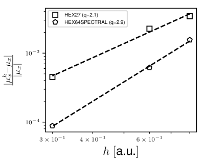
We study the rates of convergence of the dipole moment afforded by the EFE basis with respect to both spatial (FE mesh size $h$) and temporal discretization (time-step $\Delta t$), using a CO molecule of bond length 2.4 a.u. as a benchmark system. In order to reliably study the rates of convergence with respect to the mesh size, we need to mimic a semi-discrete (discrete in space but continuous in time) error analysis, so as to make the spatial discretization error to be the dominant source of error. To that end, we use a small time-step of $\Delta t=10^{-3}$ and small tolerance of $10^{-12}$ for the Krylov subspace projection error (Eq. 23). A large cubical domain of side 50 a.u. is chosen to ensure that the electron density decays to zero on the domain boundary, allowing us to impose Dirichlet boundary condition on the time-dependent Kohn-Sham orbitals and the Hartree potential. We consider two different orders ($p$) of finite elements—HEX27 ($p=2$) and HEX64SPECTRAL ($p=3$). For each $p$, we consider a sequence of increasingly refined meshes using the recipe presented in  2.7 with increasing values of $N_{\text{elem}}$. For all the meshes, we first, obtain the ground-state and then excite the system using a Gaussian electric field of the form $\textbf{E}_{0}(t)=\kappa e^{(t-t_{0})^{2}/2s^{2}}\hat{\boldsymbol{\textbf{x}}}_{1}$, with $\kappa=2\times 10^{-5}$ a.u., $t_{0}=3.0$ a.u., $s=0.2$ a.u.  and $\hat{\boldsymbol{\textbf{x}}}_{1}$ denoting the unit vector along $x$-direction. We note that the semi-discrete error in the dipole moment, as a function of the mesh size ($h$), can be expressed as ⁹⁶

$$\frac{\left|\mu_{x}(t)-\mu_{x}^{h}(t)\right|}{\left|\mu_{x}(t)\right|}=Ch^{q}\,,$$

(24)

where $\mu_{x}(t)$ and $\mu_{x}^{h}(t)$ are the continuum and discrete values of the $x$-component of the dipole moment at time $t$, $C$ is a mesh-independent constant, and $q$ is the rate of convergence. We first evaluate $\mu_{x}(t)$ using the EFE basis with a highly refined HEX125SPECTRAL ($p=4$) finite-element mesh. Subsequently, $C$ and $q$ are obtained by fitting the above relation to a set of $\mu_{x}^{h}(t)$ and $h$. Fig. 1 presents the relative semi-discrete error in the dipole moment at $t=5$ a.u.  (1 a.u. = 0.024188 fs). As evident, the numerical rates of convergence are in close agreement with the theoretical rate of $\mathcal{O}(h^{p})$, where $p$ is the order of the FE basis ($p=2$ for HEX27 and $p=3$ for HEX64SPECTRAL).

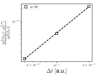
We, next, turn to the study the rate of convergence of the dipole moment with respect to temporal discretization. To this end, we used a finite element mesh with a sufficiently refined HEX125SPECTRAL mesh, such that it affords $10^{-4}$ relative error with respect to spatial discretization. We use the same Gaussian electric field as above and propagate the ground-state Kohn-Sham orbitals using second-order Magnus propagator with different $\Delta t$. The full-discrete (discrete both in space and time) error in the dipole moment at time $t_{n}$ is given as ⁹⁶

$$\frac{\left|\mu^{h}_{x}(t_{n})-\mu^{h,n}_{x}\right|}{\left|\mu^{h}_{x}(t_{n})\right|}=C(\Delta t)^{q}\,,$$

(25)

where $\mu^{h}_{x}(t_{n})$ and $\mu^{h,n}_{x}$ are the semi-discrete and full-discrete values of the $x$-component of the dipole moment at time $t_{n}$, $C$ is a constant, and $q$ is the rate of convergence. Fig.  2 depicts the rate of convergence of the dipole moment with respect to $\Delta t$ at $t_{n}=5.0$ a.u. . We attain a numerical rate of convergence of $q=1.99$, which is in good agreement with the quadratic rate of convergence for second-order Magnus propagator.

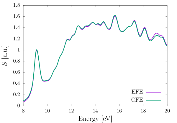
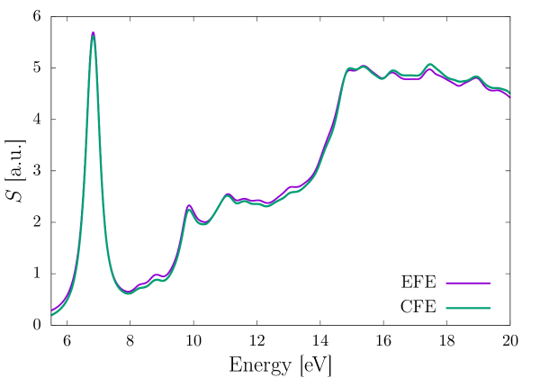
We now consider methane and benzene molecules as our benchmark systems to compare the performance of the EFE and CFE basis. For both the molecules, we excite the system from their groundstate, in each of the three directions, separately, using a weak Gaussian electric field of the form $\textbf{E}_{0}(t)=\kappa e^{-(t-t_{0})^{2}/2s^{2}}\hat{\boldsymbol{\textbf{x}}}_{j}$, with $\kappa=2\times 10^{-5}$, $t_{0}=3$, $s=0.2$ (all in a.u.), and $\hat{\boldsymbol{\textbf{x}}}_{j}$ being the unit vector along $j-$th coordinate axis. Both the systems are propagated for 20 fs. We use a third-order (HEX64SPECTRAL) and fourth-order (HEX125SPECTRAL) finite element mesh for the EFE and CFE based calculations, respectively, adaptively refined as per the strategy presented in Sec. 2.7, so as to attain 0.1 mHa accuracy in the groundstate energy per atom. Furthermore, we use a large cubical domain of length 60 a.u. and 70 a.u. for methane and benzene, respectively, to ensure that the Kohn-Sham orbitals decay to zero, and thereby, avoid any reflection effects. We chose a time-step ($\Delta t)$ of 0.1 and 0.05 a.u.  for the EFE and CFE calculations, respectively, and a Krylov subspace tolerance ($\epsilon$) of $10^{-7}$ for both the basis sets, to attain $<1$ mHa accuracy in the excitation energies. To evaluate the excitation energies, we first, take the Fourier transform of the dipole moment to obtain the dynamic polarizability, $\alpha_{i,j}(\omega)$, where $i,j$ are the index of the electric field’s polarization direction and measurement direction of the dipole, respectively. Subsequently, we compute the absorption spectrum $S(\omega)=\frac{4\omega}{3\pi}\frac{\text{Tr}\left[\text{Im}\left[\boldsymbol{\alpha}(\omega)\right]\right]}{{\mathcal{F}}\left[\textbf{E}_{0}\right](\omega)}$, where ${\mathcal{F}}\left[\textbf{E}_{0}\right](\omega)$ denotes the Fourier transform of the applied electric field $\textbf{E}_{0}(t)$. Finally, the peaks in the absorption spectrum correspond to the excitation energies. We damp the dipole moment with an exponential window of the form $g(t)=e^{-t/\tau}$, with $\tau=100$ a.u. to artificially broaden the excitation peaks. Fig. 3 and Fig. 4 compare the EFE and CFE basis based absorption spectrum for methane and benzene, respectively. We attain remarkable agreement in the absorption spectrum between the two basis, underscoring the accuracy of the EFE basis. Table 1 compares the performance of the EFE and CFE basis, in terms of the number of basis functions required and the computational cost incurred. As evident, the EFE basis attains a staggering $\sim 50\times$ and $\sim 100\times$ speedup over the CFE basis for the methane and the benzene molecule, respectively. This speedup is attributed to a combination of $3-5\times$ reduction in number of basis functions, $\sim 2\times$ reduction in the stencil of the discrete matrices (HEX64SPECTRAL in EFE and HEX125SPECTRAL in CFE), $2\times$ reduction in the time-step, and $4-5\times$ reduction in Krylov subspace size required by the EFE as compared to that of the CFE basis. Given the huge computational cost associated with the CFE basis, in the remaining benchmark calculations presented in subsequent sections, we only employ the EFE basis.

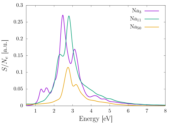
In order to demonstrate the efficacy of the EFE for larger systems, we study the absorption spectrum of three sodium clusters of increasing sizes—Na₃, Na₁₁, and Na₅₀. For all the three systems, we employ a third-order (HEX64SPECTRAL) finite element mesh that is adaptively refined using the strategy presented in Sec. 2.7 and commensurate with 0.1 mHa accuracy in the groundstate energy per atom. Furthermore, we use large cubical domains—70 a.u. for Na₃ and Na₁₁, and 85 a.u. for Na₅₀—to avoid any reflection effects from the boundary. We use the same Gaussian electric field as used in the methane and benzene benchmark calculations to excite the clusters from their groundstate and propagate the TDKS equations for 20 fs. Similar to the previous examples, we use a time-step of 0.1 a.u. and Krylov subspace tolerance of $10^{-7}$ to attain $<1$ mHa accuracy in excitation energies. Fig. 5 presents the absorption spectrum of the three sodium clusters, normalized with the number of electrons, wherein we have used an exponential window of the form $g(t)=e^{-t/\tau}$, with $\tau=200$ a.u.  to artificially broaden the excitation peaks. Table 2 provides the number of basis functions and the total computation time required by the EFE basis for the three sodium clusters. Using the timings reported, we attain a scaling of $\mathcal{O}(N_{e}^{2.01})$ with respect to the number of electrons, which agrees well with the expected quadratic scaling of the TDKS problem.

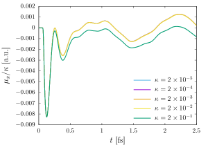
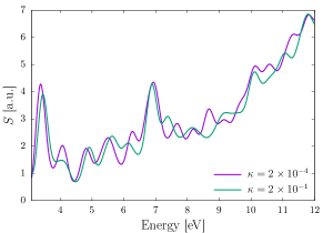
The green fluorescent protein (GFP), abundantly found in jellyfish, corals, copepods, is a commonly used tool to understand a wide array of biochemical processes ranging from fluorescence microscopy ¹¹⁵ to gene therapy ¹¹⁶ to reporter gene technology ¹¹⁷. In this example, we study the linear to nonlinear response of the chromophore of the GFP—a small molecule that lends it color. We employ a second-order (HEX27) finite element mesh that is adaptively refined using the strategy presented in Sec. 2.7 and commensurate with 0.1 mHa accuracy in the groundstate energy per atom. We use a large cubucal domain of 120 a.u. to avoid any reflection effects from the boundary. First, we identify the onset of nonlinear response by subjecting the chromophore, at its groundstate, to a series of Gaussian electric field of the form provided in Sec. 3.2 with the strength ($\kappa$) taking values of $2\times 10^{-5}$, $2\times 10^{-4}$, $2\times 10^{-3}$, $2\times 10^{-2}$, and $2\times 10^{-1}$ (all in a.u.). In linear response regime, the dipole moments scaled by the strength of the electric field are expected to be identical, and hence, can be used to identify the onset of nonlinear response. For the purpose of identifying the linear to nonlinear transition, for each of the strengths, we propagate the system for a short duration of 2.5 fs and observe the scaled dipole moment scaled. As evident from  6(a), the clear deviation of the scaled dipole moment for $\kappa=2\times 10^{-1}$ from that of the rest of the strengths, indicates the onset of nonlinear regime to be around $\kappa=2\times 10^{-1}$. Having identified the linear and nonlinear regimes, we propagate the system for longer timescale of 20 fs using a weak ($\kappa=2\times 10^{-4}$) and a strong perturbation ($\kappa=2\times 10^{-1}$). Fig. 6(b) presents a comparison of the absorption spectrum for both the strengths, where the peaks are artificially broadened with an exponential window $e^{-t/\tau}$ with $\tau=300$ a.u. . We observe the first excitation peak at $3.37$ eV, which agrees well with the experimental value of 3.51 eV ¹¹⁸. As evident, the strong perturbation has a decreased height of the first absorption peak, largely owing to saturation effect (i.e., the inability of the highly excited molecule under strong perturbation to absorb subsequent radiations). Furthermore, for the strong perturbation, we observe a blue-shifting of the absorption peaks in the lower energy ($<6$ eV) regime. In the higher energy regime ($>6$ eV), for the strong perturbation, we observe fewer excitation peaks, indicating the absorption to be spread over a range of frequencies. We remark that, despite the use of strong perturbation and large domain size, we require only $\sim 18,000$ basis functions per atom, highlighting the efficiency of the EFE basis even for strong perturbations in TDDFT.

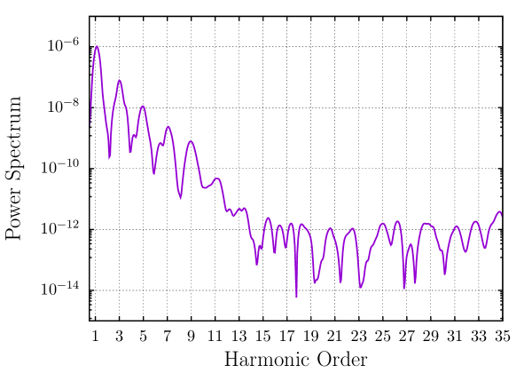
We examine the competence of the EFE basis for simulating strong perturbations by studying the higher harmonic generation in a magnesium dimer with a bond-length of $4.74$ a.u. . We use a strong sinusoidal electric field of the form $\textbf{E}_{0}(t)=\kappa\text{sin}(\pi t/T)\text{sin}(\omega t)\hat{\boldsymbol{\textbf{x}}}_{1}$, with $\kappa=0.01$, $\omega=0.03$, and $T=5\times(2\pi/\omega)$ (all in a.u.) to excite the system from its groundstate and propagate for $T$ fs. For an efficient choice of finite element mesh, we employ adaptive third-order (HEX64SPECTRAL) finite elements, obtained using the approach presented in Sec. 2.7. As with previous examples, we use a cubical domain of length 100 a.u. to eliminate any reflection effects from the boundaries. We employ a time-step of 0.1 a.u. and a Krylov subspace tolerance of $10^{-7}$. Fig. 7 shows the dipole power spectrum ($P(\omega)$) for Mg₂, defined as $P(\omega)=\left|\int_{0}^{T}e^{-i\omega t}\frac{d}{dt^{2}}\mu_{x}(t)dt\right|^{2}$ (i.e., square of the Fourier transform of the acceleration of the dipole moment). We have artificially broadened the peaks by using a gaussian window of form $e^{-t^{2}/\tau}$, with $\tau=10^{5}$ a.u. . For a system with spatial inversion symmetry, only odd multiples of the frequency of the exciting laser pulse must be emitted, which is well verified in Fig. 7 with the peaks in the power spectrum coinciding with odd harmonics (odd multiples of $\omega$). We also observe that the rate of decay of the intensity of the peaks flattens beyond the $13$-$th$ harmonic, which corroborates well with the plateau phenomenon observed in experiments ¹¹⁹. Despite the large domain size used in this calculation, we require only $\sim 32,000$ basis functions per atom, further underscoring the efficiency of the EFE basis even for strong perturbations in TDDFT.

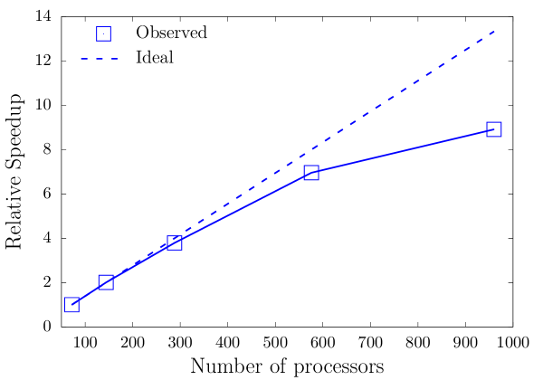
Finally, we examine the parallel scalability of the implementation of our EFE basis for TDDFT calculations, using the Na₅₀ cluster with $~{}\sim 1.7$ million basis functions as a benchmark system. We repeat the same calculation as presented in Sec. 3.3 and measure the relative speedup in the walltime with respect to 72 processors. As evident from Fig. 8, we attain close to ideal scaling until 576 processors, at which we observe a parallel efficiency of 87%. The efficiency drops to 67% at 960 processors owing to fact that, at 960 processors, the number of basis functions per processor falls below 2000, which is low to sustain good parallel scalability.

References

- Hohenberg and Kohn 1964 Hohenberg, P.; Kohn, W. Inhomogeneous Electron Gas. Phys. Rev. 1964, 136, B864–B871
- Runge and Gross 1984 Runge, E.; Gross, E. K. U. Density-Functional Theory for Time-Dependent Systems. Phys. Rev. Lett. 1984, 52, 997–1000
- Van Leeuwen 1999 Van Leeuwen, R. Mapping from densities to potentials in time-dependent density-functional theory. Physical review letters 1999, 82, 3863
- Appel et al. 2003 Appel, H.; Gross, E. K. U.; Burke, K. Excitations in Time-Dependent Density-Functional Theory. Phys. Rev. Lett. 2003, 90, 043005
- Gonze and Vigneron 1989 Gonze, X.; Vigneron, J.-P. Density-functional approach to nonlinear-response coefficients of solids. Phys. Rev. B 1989, 39, 13120–13128
- van Gisbergen et al. 1997 van Gisbergen, S. J. A.; Snijders, J. G.; Baerends, E. J. Time-dependent Density Functional Results for the Dynamic Hyperpolarizability of . Phys. Rev. Lett. 1997, 78, 3097–3100
- Tong and Chu 1998 Tong, X.-M.; Chu, S.-I. Time-dependent density-functional theory for strong-field multiphoton processes: Application to the study of the role of dynamical electron correlation in multiple high-order harmonic generation. Phys. Rev. A 1998, 57, 452–461
- Chu and Chu 2001 Chu, X.; Chu, S.-I. Time-dependent density-functional theory for molecular processes in strong fields: Study of multiphoton processes and dynamical response of individual valence electrons of N2 in intense laser fields. Physical Review A 2001, 64, 063404
- Tong and Chu 2001 Tong, X.-M.; Chu, S.-I. Multiphoton ionization and high-order harmonic generation of He, Ne, and Ar atoms in intense pulsed laser fields: Self-interaction-free time-dependent density-functional theoretical approach. Phys. Rev. A 2001, 64, 013417
- Telnov and Chu 2009 Telnov, D. A.; Chu, S.-I. Effects of electron structure and multielectron dynamical response on strong-field multiphoton ionization of diatomic molecules with arbitrary orientation: An all-electron time-dependent density-functional-theory approach. Phys. Rev. A 2009, 79, 041401
- Dauth et al. 2016 Dauth, M.; Graus, M.; Schelter, I.; Wießner, M.; Schöll, A.; Reinert, F.; Kümmel, S. Perpendicular emission, dichroism, and energy dependence in angle-resolved photoemission: the importance of the final state. Physical Review Letters 2016, 117, 183001
- Hatcher et al. 2008 Hatcher, R.; Beck, M.; Tackett, A.; Pantelides, S. T. Dynamical effects in the interaction of ion beams with solids. Physical review letters 2008, 100, 103201
- Yost et al. 2019 Yost, D. C.; Yao, Y.; Kanai, Y. First-principles modeling of electronic stopping in complex matter under ion irradiation. The Journal of Physical Chemistry Letters 2019, 11, 229–237
- Pruneda et al. 2007 Pruneda, J.; Sánchez-Portal, D.; Arnau, A.; Juaristi, J.; Artacho, E. Electronic stopping power in LiF from first principles. Physical review letters 2007, 99, 235501
- Correa et al. 2012 Correa, A. A.; Kohanoff, J.; Artacho, E.; Sánchez-Portal, D.; Caro, A. Nonadiabatic forces in ion-solid interactions: the initial stages of radiation damage. Physical review letters 2012, 108, 213201
- Schleife et al. 2015 Schleife, A.; Kanai, Y.; Correa, A. A. Accurate atomistic first-principles calculations of electronic stopping. Physical Review B 2015, 91, 014306
- Lopata et al. 2012 Lopata, K.; Van Kuiken, B. E.; Khalil, M.; Govind, N. Linear-response and real-time time-dependent density functional theory studies of core-level near-edge x-ray absorption. Journal of chemical theory and computation 2012, 8, 3284–3292
- Attar et al. 2017 Attar, A. R.; Bhattacherjee, A.; Pemmaraju, C.; Schnorr, K.; Closser, K. D.; Prendergast, D.; Leone, S. R. Femtosecond x-ray spectroscopy of an electrocyclic ring-opening reaction. Science 2017, 356, 54–59
- Pemmaraju et al. 2018 Pemmaraju, C. D.; Vila, F. D.; Kas, J. J.; Sato, S. A.; Rehr, J. J.; Yabana, K.; Prendergast, D. Velocity-gauge real-time TDDFT within a numerical atomic orbital basis set. Comput. Phys. Commun. 2018, 226, 30–38
- Pemmaraju 2019 Pemmaraju, C. Valence and core excitons in solids from velocity-gauge real-time TDDFT with range-separated hybrid functionals: An LCAO approach. Computational Condensed Matter 2019, 18, e00348
- Yao et al. 2019 Yao, Y.; Yost, D. C.; Kanai, Y. K-shell core-electron excitations in electronic stopping of protons in water from first principles. Physical Review Letters 2019, 123, 066401
- Ma et al. 2015 Ma, J.; Wang, Z.; Wang, L.-W. Interplay between plasmon and single-particle excitations in a metal nanocluster. Nature communications 2015, 6, 1–11
- Peng et al. 2015 Peng, B.; Lingerfelt, D. B.; Ding, F.; Aikens, C. M.; Li, X. Real-time TDDFT studies of exciton decay and transfer in silver nanowire arrays. The Journal of Physical Chemistry C 2015, 119, 6421–6427
- Mrudul et al. 2020 Mrudul, M.; Tancogne-Dejean, N.; Rubio, A.; Dixit, G. High-harmonic generation from spin-polarised defects in solids. npj Computational Materials 2020, 6, 1–9
- Tancogne-Dejean et al. 2017 Tancogne-Dejean, N.; Mücke, O. D.; Kärtner, F. X.; Rubio, A. Impact of the electronic band structure in high-harmonic generation spectra of solids. Physical review letters 2017, 118, 087403
- Stefanucci and Almbladh 2004 Stefanucci, G.; Almbladh, C.-O. Time-dependent quantum transport: An exact formulation based on TDDFT. EPL 2004, 67, 14
- Kurth et al. 2005 Kurth, S.; Stefanucci, G.; Almbladh, C.-O.; Rubio, A.; Gross, E. K. U. Time-dependent quantum transport: A practical scheme using density functional theory. Phys. Rev. B 2005, 72, 035308
- Jamorski Jödicke and Lüthi 2003 Jamorski Jödicke, C.; Lüthi, H. P. Time-Dependent Density Functional Theory (TDDFT) Study of the Excited Charge-Transfer State Formation of a Series of Aromatic donor–acceptor Systems. J. Am. Chem. Soc. 2003, 125, 252–264
- Stein et al. 2009 Stein, T.; Kronik, L.; Baer, R. Reliable prediction of charge transfer excitations in molecular complexes using time-dependent density functional theory. J. Am. Chem. Soc. 2009, 131, 2818–2820
- Burnus et al. 2005 Burnus, T.; Marques, M. A. L.; Gross, E. K. U. Time-dependent electron localization function. Phys. Rev. A 2005, 71, 010501
- Abu-Jafar et al. 2000 Abu-Jafar, M.; Al-Sharif, A.; Qteish, A. FP-LAPW and pseudopotential calculations of the structural phase transformations of GaN under high-pressure. Solid State Communications 2000, 116, 389–393
- Oganov and Dorogokupets 2003 Oganov, A. R.; Dorogokupets, P. I. All-electron and pseudopotential study of MgO: Equation of state, anharmonicity, and stability. Phys. Rev. B 2003, 67, 224110
- Kolorenč and Mitas 2007 Kolorenč, J. c. v.; Mitas, L. -to- structural phase transition in MnO under pressure: Comparison of all-electron and pseudopotential approaches. Phys. Rev. B 2007, 75, 235118
- Xiao et al. 2010 Xiao, H. Y.; Jiang, X.; Duan, G.; Gao, F.; Zu, X. T.; Weber, W. J. First-principles calculations of pressure-induced phase transformation in AlN and GaN. Computational materials science 2010, 48, 768–772
- Liu et al. 1998 Liu, W.; Küchle, W.; Dolg, M. Ab initio pseudopotential and density-functional all-electron study of ionization and excitation energies of actinide atoms. Phys. Rev. A 1998, 58, 1103–1110
- Schwerdtfeger et al. 2011 Schwerdtfeger, P.; Assadollahzadeh, B.; Rohrmann, U.; Schäfer, R.; Cheeseman, J. R. Breakdown of the pseudopotential approximation for magnetizabilities and electric multipole moments: Test calculations for Au, AuF, and Sn n cluster (n¡=20). The Journal of chemical physics 2011, 134, 204102
- Schwerdtfeger et al. 1995 Schwerdtfeger, P.; Fischer, T.; Dolg, M.; Igel-Mann, G.; Nicklass, A.; Stoll, H.; Haaland, A. The accuracy of the pseudopotential approximation. I. An analysis of the spectroscopic constants for the electronic ground states of InCl and InCl3 using various three valence electron pseudopotentials for indium. The Journal of chemical physics 1995, 102, 2050–2062
- Leininger et al. 1996 Leininger, T.; Nicklass, A.; Stoll, H.; Dolg, M.; Schwerdtfeger, P. The accuracy of the pseudopotential approximation. II. A comparison of various core sizes for indium pseudopotentials in calculations for spectroscopic constants of InH, InF, and InCl. The Journal of chemical physics 1996, 105, 1052–1059
- Schwerdtfeger et al. 2000 Schwerdtfeger, P.; Brown, J. R.; Laerdahl, J. K.; Stoll, H. The accuracy of the pseudopotential approximation. III. A comparison between pseudopotential and all-electron methods for Au and AuH. The Journal of Chemical Physics 2000, 113, 7110–7118
- Gómez-Abal et al. 2008 Gómez-Abal, R.; Li, X.; Scheffler, M.; Ambrosch-Draxl, C. Influence of the Core-Valence Interaction and of the Pseudopotential Approximation on the Electron Self-Energy in Semiconductors. Phys. Rev. Lett. 2008, 101, 106404
- Govoni and Galli 2018 Govoni, M.; Galli, G. GW100: comparison of methods and accuracy of results obtained with the WEST code. Journal of chemical theory and computation 2018, 14, 1895–1909
- Casida 1995 Casida, M. E. Recent Advances In Density Functional Methods: (Part I); World Scientific, 1995
- Petersilka et al. 1996 Petersilka, M.; Gossmann, U. J.; Gross, E. K. U. Excitation Energies from Time-Dependent Density-Functional Theory. Phys. Rev. Lett. 1996, 76, 1212–1215
- Mortensen et al. 2005 Mortensen, J. J.; Hansen, L. B.; Jacobsen, K. W. Real-space grid implementation of the projector augmented wave method. Phys. Rev. B 2005, 71, 035109
- Schleife et al. 2012 Schleife, A.; Draeger, E. W.; Kanai, Y.; Correa, A. A. Plane-wave pseudopotential implementation of explicit integrators for time-dependent Kohn-Sham equations in large-scale simulations. J. Chem. Phys. 2012, 137, 22A546
- Soler et al. 2002 Soler, J. M.; Artacho, E.; Gale, J. D.; García, A.; Junquera, J.; Ordejón, P.; Sánchez-Portal, D. The SIESTA method for ab initio order-N materials simulation. J. Phys.: Condens. Matter 2002, 14, 2745
- Takimoto et al. 2007 Takimoto, Y.; Vila, F. D.; Rehr, J. J. Real-time time-dependent density functional theory approach for frequency-dependent nonlinear optical response in photonic molecules. J. Chem. Phys. 2007, 127, 154114
- Kuisma et al. 2015 Kuisma, M.; Sakko, A.; Rossi, T. P.; Larsen, A. H.; Enkovaara, J.; Lehtovaara, L.; Rantala, T. T. Localized surface plasmon resonance in silver nanoparticles: Atomistic first-principles time-dependent density-functional theory calculations. Phys. Rev. B 2015, 91, 115431
- Valiev et al. 2010 Valiev, M.; Bylaska, E.; Govind, N.; Kowalski, K.; Straatsma, T.; Dam, H. V.; Wang, D.; Nieplocha, J.; Apra, E.; Windus, T.; de Jong, W. NWChem: A comprehensive and scalable open-source solution for large scale molecular simulations. Comput. Phys. Commun. 2010, 181, 1477–1489
- Lopata and Govind 2011 Lopata, K.; Govind, N. Modeling fast electron dynamics with real-time time-dependent density functional theory: application to small molecules and chromophores. J. Chem. Theory Comput. 2011, 7, 1344–1355
- Blum et al. 2009 Blum, V.; Gehrke, R.; Hanke, F.; Havu, P.; Havu, V.; Ren, X.; Reuter, K.; Scheffler, M. Ab initio molecular simulations with numeric atom-centered orbitals. Comput. Phys. Commun. 2009, 180, 2175–2196
- Hekele et al. 2021 Hekele, J.; Yao, Y.; Kanai, Y.; Blum, V.; Kratzer, P. All-electron real-time and imaginary-time time-dependent density functional theory within a numeric atom-centered basis function framework. The Journal of Chemical Physics 2021, 155, 154801
- Gulans et al. 2014 Gulans, A.; Kontur, S.; Meisenbichler, C.; Nabok, D.; Pavone, P.; Rigamonti, S.; Sagmeister, S.; Werner, U.; Draxl, C. Exciting: a full-potential all-electron package implementing density-functional theory and many-body perturbation theory. Journal of Physics: Condensed Matter 2014, 26, 363202
- Pela and Draxl 2021 Pela, R. R.; Draxl, C. All-electron full-potential implementation of real-time TDDFT in exciting. Electronic Structure 2021, 3, 037001
- 55 The Elk Code. http://elk.sourceforge.net/
- Castro et al. 2006 Castro, A.; Appel, H.; Oliveira, M.; Rozzi, C. A.; Andrade, X.; Lorenzen, F.; Marques, M. A. L.; Gross, E. K. U.; Rubio, A. octopus: a tool for the application of time-dependent density functional theory. Phys. Status Solidi B 2006, 243, 2465–2488
- Walter et al. 2008 Walter, M.; Häkkinen, H.; Lehtovaara, L.; Puska, M.; Enkovaara, J.; Rostgaard, C.; Mortensen, J. J. Time-dependent density-functional theory in the projector augmented-wave method. J. Chem. Phys. 2008, 128, 244101
- Slater 1964 Slater, J. Advances in quantum chemistry; Elsevier, 1964; Vol. 1; pp 35–58
- Singh and Nordstrom 2006 Singh, D. J.; Nordstrom, L. Planewaves, Pseudopotentials, and the LAPW method; Springer Science & Business Media, 2006
- Loucks 1967 Loucks, T. L. Augmented Plane Wave Method: A Guide to Performing Electronic Structure Calculations; Frontiers in Physics: Lecture note and reprint series, A; Benjamin, 1967
- Koelling and Arbman 1975 Koelling, D. D.; Arbman, G. O. Use of energy derivative of the radial solution in an augmented plane wave method: application to copper. Journal of Physics F: Metal Physics 1975, 5, 2041
- Andersen 1975 Andersen, O. K. Linear methods in band theory. Physical Review B 1975, 12, 3060
- Wimmer et al. 1981 Wimmer, E.; Krakauer, H.; Weinert, M.; Freeman, A. J. Full-potential self-consistent linearized-augmented-plane-wave method for calculating the electronic structure of molecules and surfaces: molecule. Phys. Rev. B 1981, 24, 864–875
- Weinert et al. 1982 Weinert, M.; Wimmer, E.; Freeman, A. J. Total-energy all-electron density functional method for bulk solids and surfaces. Phys. Rev. B 1982, 26, 4571–4578
- Sjöstedt et al. 2000 Sjöstedt, E.; Nordström, L.; Singh, D. J. An alternative way of linearizing the augmented plane-wave method. Solid state communications 2000, 114, 15–20
- Madsen et al. 2001 Madsen, G. K. H.; Blaha, P.; Schwarz, K.; Sjöstedt, E.; Nordström, L. Efficient linearization of the augmented plane-wave method. Phys. Rev. B 2001, 64, 195134
- Singh 1991 Singh, D. Ground-state properties of lanthanum: Treatment of extended-core states. Physical Review B 1991, 43, 6388
- Schwarz et al. 2002 Schwarz, K.; Blaha, P.; Madsen, G. K. Electronic structure calculations of solids using the WIEN2k package for material sciences. Comput. Phys. Commun. 2002, 147, 71–76
- Vignale 2004 Vignale, G. Mapping from current densities to vector potentials in time-dependent current density functional theory. Physical Review B 2004, 70, 201102
- Jensen et al. 2017 Jensen, S. R.; Saha, S.; Flores-Livas, J. A.; Huhn, W.; Blum, V.; Goedecker, S.; Frediani, L. The Elephant in the Room of Density Functional Theory Calculations. The Journal of Physical Chemistry Letters 2017, 8, 1449–1457, PMID: 28291362
- Jensen 2017 Jensen, F. How Large is the Elephant in the Density Functional Theory Room? The Journal of Physical Chemistry A 2017, 121, 6104–6107, PMID: 28722449
- Feller and Dixon 2018 Feller, D.; Dixon, D. A. Density Functional Theory and the Basis Set Truncation Problem with Correlation Consistent Basis Sets: Elephant in the Room or Mouse in the Closet? The Journal of Physical Chemistry A 2018, 122, 2598–2603, PMID: 29462560
- Brenner and Scott 2007 Brenner, S.; Scott, R. The mathematical theory of finite element methods; Springer Science & Business Media, 2007; Vol. 15
- Hughes 2012 Hughes, T. J. R. The finite element method: linear static and dynamic finite element analysis; Courier Corporation, 2012
- White et al. 1989 White, S. R.; Wilkins, J. W.; Teter, M. P. Finite-element method for electronic structure. Phys. Rev. B 1989, 39, 5819–5833
- Tsuchida and Tsukada 1998 Tsuchida, E.; Tsukada, M. Large-Scale Electronic-Structure Calculations Based on the Adaptive Finite-Element Method. Journal of the Physical Society of Japan 1998, 67, 3844–3858
- Pask et al. 1999 Pask, J. E.; Klein, B. M.; Fong, C. Y.; Sterne, P. A. Real-space local polynomial basis for solid-state electronic-structure calculations: A finite-element approach. Phys. Rev. B 1999, 59, 12352–12358
- Pask et al. 2001 Pask, J. E.; Klein, B. M.; Sterne, P. A.; Fong, C. Y. Finite-element methods in electronic-structure theory. Comput. Phys. Commun. 2001, 135, 1 – 34
- Pask and Sterne 2005 Pask, J. E.; Sterne, P. A. Finite element methods in ab initio electronic structure calculations. Modelling and Simulation in Materials Science and Engineering 2005, 13, R71–R96
- Zhang et al. 2008 Zhang, D.; Shen, L.; Zhou, A.; Gong, X.-G. Finite element method for solving Kohn–Sham equations based on self-adaptive tetrahedral mesh. Physics Letters A 2008, 372, 5071 – 5076
- Suryanarayana et al. 2010 Suryanarayana, P.; Gavini, V.; Blesgen, T.; Bhattacharya, K.; Ortiz, M. Non-periodic finite-element formulation of Kohn–Sham density functional theory. Journal of the Mechanics and Physics of Solids 2010, 58, 256 – 280
- Fang et al. 2012 Fang, J.; Gao, X.; Zhou, A. A Kohn–Sham equation solver based on hexahedral finite elements. Journal of Computational Physics 2012, 231, 3166 – 3180
- Bao et al. 2012 Bao, G.; Hu, G.; Liu, D. An h-adaptive finite element solver for the calculations of the electronic structures. Journal of Computational Physics 2012, 231, 4967 – 4979
- Motamarri et al. 2013 Motamarri, P.; Nowak, M. R.; Leiter, K.; Knap, J.; Gavini, V. Higher-order adaptive finite-element methods for Kohn–Sham density functional theory. Journal of Computational Physics 2013, 253, 308–343
- Motamarri and Gavini 2018 Motamarri, P.; Gavini, V. Configurational forces in electronic structure calculations using Kohn-Sham density functional theory. Phys. Rev. B 2018, 97, 165132
- Das et al. 2019 Das, S.; Motamarri, P.; Gavini, V.; Turcksin, B.; Li, Y. W.; Leback, B. Fast, scalable and accurate finite-element based ab initio calculations using mixed precision computing: 46 PFLOPS simulation of a metallic dislocation system. Proceedings of the International Conference for High Performance Computing, Networking, Storage and Analysis. 2019; pp 1–11
- Motamarri et al. 2020 Motamarri, P.; Das, S.; Rudraraju, S.; Ghosh, K.; Davydov, D.; Gavini, V. DFT-FE–A massively parallel adaptive finite-element code for large-scale density functional theory calculations. Comput. Phys. Commun. 2020, 246, 106853
- Das et al. 2022 Das, S.; Motamarri, P.; Subramanian, V.; Rogers, D. M.; Gavini, V. DFT-FE 1.0: A massively parallel hybrid CPU-GPU density functional theory code using finite-element discretization. Comput. Phys. Commun. 2022, 280, 108473
- Zhuravel et al. 2020 Zhuravel, R.; Huang, H.; Polycarpou, G.; Polydorides, S.; Motamarri, P.; Katrivas, L.; Rotem, D.; Sperling, J.; Zotti, L. A.; Kotlyar, A. B.; Cuevas, J. C.; Gavini, V.; Skourtis, S. S.; Porath, D. Backbone charge transport in double-stranded DNA. Nat. Nanotechnol. 2020, 15, 836–840
- Ghosh et al. 2021 Ghosh, K.; Ma, H.; Onizhuk, M.; Gavini, V.; Galli, G. Spin–spin interactions in defects in solids from mixed all-electron and pseudopotential first-principles calculations. npj Comput. Mater. 2021, 7, 123
- Yao et al. 2022 Yao, L.; Das, S.; Liu, X.; Cheng, Y.; Gavini, V.; Xiao, B. Modulating the microscopic lattice distortions through the Al-rich layers for boosting the ferroelectricity in nanofilms. J. Phys. D: Appl. Phys. 2022, 55, 455501
- Kanungo et al. 2019 Kanungo, B.; Zimmerman, P. M.; Gavini, V. Exact exchange-correlation potentials from ground-state electron densities. Nat. Commun. 2019, 10, 4497
- Kanungo et al. 2021 Kanungo, B.; Zimmerman, P. M.; Gavini, V. A Comparison of exact and model exchange–correlation potentials for molecules. J. Phys. Chem. Lett. 2021, 12, 12012–12019
- Lehtovaara et al. 2011 Lehtovaara, L.; Havu, V.; Puska, M. All-electron time-dependent density functional theory with finite elements: Time-propagation approach. J. Chem. Phys. 2011, 135, 154104
- Bao et al. 2015 Bao, G.; Hu, G.; Liu, D. Real-time adaptive finite element solution of time-dependent Kohn–Sham equation. J. Comput. Phys. 2015, 281, 743–758
- Kanungo and Gavini 2019 Kanungo, B.; Gavini, V. Real time time-dependent density functional theory using higher order finite-element methods. Physical Review B 2019, 100, 115148
- Kanungo and Gavini 2017 Kanungo, B.; Gavini, V. Large-scale all-electron density functional theory calculations using an enriched finite-element basis. Physical Review B 2017, 95, 035112
- Rufus et al. 2021 Rufus, N. D.; Kanungo, B.; Gavini, V. Fast and robust all-electron density functional theory calculations in solids using orthogonalized enriched finite elements. Physical Review B 2021, 104, 085112
- Rufus and Gavini 2022 Rufus, N. D.; Gavini, V. Ionic forces and stress tensor in all-electron density functional theory calculations using an enriched finite-element basis. Physical Review B 2022, 106, 085108
- Vignale 1995 Vignale, G. Center of Mass and Relative Motion in Time Dependent Density Functional Theory. Phys. Rev. Lett. 1995, 74, 3233–3236
- Maitra et al. 2002 Maitra, N. T.; Burke, K.; Woodward, C. Memory in Time-Dependent Density Functional Theory. Phys. Rev. Lett. 2002, 89, 023002
- Marques et al. 2006 Marques, M. A. L.; Ullrich, C. A.; Nogueira, F.; Rubio, A.; Burke, K.; Gross, E. K. U. Time-dependent density functional theory; Springer: Berlin Heidelberg, 2006
- Gross and Kohn 1985 Gross, E. K. U.; Kohn, W. Local density-functional theory of frequency-dependent linear response. Phys. Rev. Lett. 1985, 55, 2850–2852
- Ceperley and Alder 1980 Ceperley, D. M.; Alder, B. J. Ground State of the Electron Gas by a Stochastic Method. Phys. Rev. Lett. 1980, 45, 566–569
- Motamarri et al. 2012 Motamarri, P.; Iyer, M.; Knap, J.; Gavini, V. Higher-order adaptive finite-element methods for orbital-free density functional theory. Journal of Computational Physics 2012, 231, 6596 – 6621
- Löwdin 1950 Löwdin, P.-O. On the non-orthogonality problem connected with the use of atomic wave functions in the theory of molecules and crystals. The Journal of Chemical Physics 1950, 18, 365–375
- Jansík et al. 2007 Jansík, B.; Høst, S.; Jørgensen, P.; Olsen, J.; Helgaker, T. Linear-scaling symmetric square-root decomposition of the overlap matrix. The Journal of Chemical Physics 2007, 126
- Niklasson 2004 Niklasson, A. M. N. Iterative refinement method for the approximate factorization of a matrix inverse. Phys. Rev. B 2004, 70, 193102
- Higham 1997 Higham, N. J. Stable iterations for the matrix square root. Numerical Algorithms 1997, 15, 227–242
- Mousavi et al. 2012 Mousavi, S. E.; Pask, J. E.; Sukumar, N. Efficient adaptive integration of functions with sharp gradients and cusps in n-dimensional parallelepipeds. International Journal for Numerical Methods in Engineering 2012, 91, 343–357
- Blanes et al. 2009 Blanes, S.; Casas, F.; Oteo, J.; Ros, J. The Magnus expansion and some of its applications. Phys. Rep. 2009, 470, 151–238
- Hochbruck and Lubich 2003 Hochbruck, M.; Lubich, C. On Magnus Integrators for Time-Dependent Schrödinger Equations. SIAM J. Numer. Anal. 2003, 41, 945–963
- Cheng et al. 2006 Cheng, C.-L.; Evans, J. S.; Van Voorhis, T. Simulating molecular conductance using real-time density functional theory. Phys. Rev. B 2006, 74, 155112
- Hochbruck et al. 1998 Hochbruck, M.; Lubich, C.; Selhofer, H. Exponential integrators for large systems of differential equations. SIAM J. Sci. Comput. 1998, 19, 1552–1574
- Bastiaens and Pepperkok 2000 Bastiaens, P. I.; Pepperkok, R. Observing proteins in their natural habitat: the living cell. Trends in biochemical sciences 2000, 25, 631–637
- Wahlfors et al. 2001 Wahlfors, J.; Loimas, S.; Pasanen, T.; Hakkarainen, T. Green fluorescent protein (GFP) fusion constructs in gene therapy research. Histochemistry and cell biology 2001, 115, 59–65
- Naylor 1999 Naylor, L. H. Reporter gene technology: the future looks bright. Biochemical pharmacology 1999, 58, 749–757
- Dong et al. 2006 Dong, J.; Solntsev, K. M.; Tolbert, L. M. Solvatochromism of the green fluorescence protein chromophore and its derivatives. Journal of the American Chemical Society 2006, 128, 12038–12039
- Brabec and Krausz 2000 Brabec, T.; Krausz, F. Intense few-cycle laser fields: Frontiers of nonlinear optics. Rev. Mod. Phys. 2000, 72, 545