Efficient and Convergent Sequential Pseudo-Likelihood Estimation of Dynamic Discrete Games
Abstract
We propose a new sequential Efficient Pseudo-Likelihood (-EPL) estimator for dynamic discrete choice games of incomplete information. -EPL considers the joint behavior of multiple players simultaneously, as opposed to individual responses to other agents’ equilibrium play. This, in addition to reframing the problem from conditional choice probability (CCP) space to value function space, yields a computationally tractable, stable, and efficient estimator. We show that each iteration in the -EPL sequence is consistent and asymptotically efficient, so the first-order asymptotic properties do not vary across iterations. Furthermore, we show the sequence achieves higher-order equivalence to the finite-sample maximum likelihood estimator with iteration and that the sequence of estimators converges almost surely to the maximum likelihood estimator at a nearly-superlinear rate when the data are generated by any regular Markov perfect equilibrium, including equilibria that lead to inconsistency of other sequential estimators. When utility is linear in parameters, -EPL iterations are computationally simple, only requiring that the researcher solve linear systems of equations to generate pseudo-regressors which are used in a static logit/probit regression. Monte Carlo simulations demonstrate the theoretical results and show -EPL’s good performance in finite samples in both small- and large-scale games, even when the game admits spurious equilibria in addition to one that generated the data. We apply the estimator analyze competition in the U.S. wholesale club industry.
Keywords: dynamic discrete games, dynamic discrete choice, multiple equilibria, pseudo maximum likelihood estimation.
JEL Classification: C57, C63, C73, L13.
1 Introduction
Estimation of dynamic discrete choice models – particularly dynamic discrete games of incomplete information – is a topic of considerable interest in economics. Broadly, likelihood-based estimation of these models takes the form
| s.t. |
where is the log-likelihood function based on independent markets, is a finite-dimensional vector of parameters, is a vector of important auxiliary parameters, and is a vector equality constraint that represents equilibrium conditions. The parameters usually consist of the structural parameters of the model. Common examples of auxiliary parameters include expected/integrated value functions or conditional choice probabilities, since the equality constraint is often derived from an equilibrium fixed point condition of the form .
One approach to estimating these models is to directly impose the fixed point equation for each trial value of visited by the optimization algorithm by solving for such that . This approach was pioneered by Miller (1984), Wolpin (1984), Pakes (1986), and Rust (1987) for single-agent models, where the fixed point is unique and can be computed via standard value function iteration or backwards induction. Solution algorithms are available for dynamic games (Pakes and McGuire, 1994, 2001), but it is often infeasible to nest those within an estimation routine because the computational burden can be quite large. Furthermore, in games the model may be incomplete due to multiple solutions (Tamer, 2003).
These issues with the nested fixed-point approach led researchers to extend conditional choice probability (CCP) estimators – first introduced in the seminal work of Hotz and Miller (1993) for single-agent models – to the case of dynamic discrete games. Of particular interest here is the nested pseudo-likelihood approach of Aguirregabiria and Mira (2002; 2007).111Some other examples of CCP estimators are described in Hotz et al. (1994); Bajari et al. (2007); Pakes et al. (2007); Pesendorfer and Schmidt-Dengler (2008). They suggest using a -step nested pseudo-likelihood (-NPL) approach, which defines a sequence of estimators, as an algorithm for computing the nested pseudo-likelihood (NPL) estimator, a fixed point of the sequence. In single-agent models, Aguirregabiria and Mira (2002) show that the -NPL estimator is efficient for when initialized with a consistent CCP estimate, in the sense that it has the same limiting distribution as the (partial) maximum likelihood estimator. Furthermore, Kasahara and Shimotsu (2008) showed that the sequence converges to the true parameter values with probability approaching one in large samples. Indeed, the Monte Carlo simulations in Aguirregabiria and Mira (2002) show that single-agent -NPL reliably converges to the maximum likelihood estimate. The combination of computational simplicity, efficiency, and convergence stability make -NPL an attractive alternative to other approaches, such as nested fixed point (computationally burdensome) or standard Newton or Fisher scoring steps on the full maximum likelihood problem (often diverges in finite samples in practice).222This is a well-known limitation of standard Newton steps, and further regularization is often needed to ensure convergence.
Unfortunately, these attractive properties of -NPL are lost in dynamic games. Aguirregabiria and Mira (2007) show that -NPL estimates are in general not efficient for , although they show that the -NPL (taking or until convergence) estimator outperforms the -NPL estimator in efficiency when both are consistent. But Pesendorfer and Schmidt-Dengler (2010) show that the sequence may fail to converge to the equilibrium that generated the data, even with very good starting values, so that -NPL may not be consistent (see also, Kasahara and Shimotsu (2012), Egesdal et al. (2015), and Aguirregabiria and Marcoux (2021)). Kasahara and Shimotsu (2012) show that inconsistency occurs when the NPL mapping is unstable at the data-generating equilibrium, which is essentially equivalent to best-response instability of the equilibrium.333The NPL mapping is first-order equivalent to the best-response mapping at the equilibrium.
Another type of CCP estimator is the minimum-distance estimator (Altug and Miller (1998); Pesendorfer and Schmidt-Dengler (2008)). This estimator is both consistent and efficient in dynamic games, and Bugni and Bunting (2021) develop a sequential version of this estimator, which we refer to as -MD. However, Monte Carlo simulations show that these econometric properties come at the expense of greatly increased computational burden, taking 12 to 26 times longer per iteration than -NPL in even the simplest small-scale dynamic games.444Bugni and Bunting (2021) perform Monte Carlo simulations with a very small-scale game (two players, two actions, four states), and even in that setting they remark, “… computing the optimally weighted 1-MD, 2-MD, and 3-MD estimators takes us roughly 33%, 75%, and 80% more time than computing the 20-[NPL] estimator, respectively.” These translate to roughly 26, 17.5, and 12 times longer per iteration for each respective case. This difference in computation time is likely to grow with the size of the game, which would be a serious concern for empirical applications. This leaves the researcher with an undesirable tradeoff between the computationally simple -NPL sequence and the more burdensome -MD sequence with better efficiency properties.
But there is another concern shared by the -NPL and -MD sequences: finite sample performance of successive iterations. The -MD estimator uses the NPL mapping to update choice probabilities between iterations, so there is reason to be concerned that it may mimic -NPL’s finite sample properties when the data-generating equilibrium is NPL-unstable. While the first-order asymptotic analysis of Bugni and Bunting (2021) implies that both sequences are consistent for finite , this asymptotic consistency does not necessarily lead to good performance in finite samples. Indeed, the finite-sample performance of -NPL deteriorates with when the equilibrium is NPL-unstable. For example, Pesendorfer and Schmidt-Dengler (2008) consider a finite number of iterations for -NPL and find that it is severely biased in large-but-finite samples when the equilibrium is NPL-unstable. In our own Monte Carlo simulations presented later, we find that substantial bias appears rather quickly, even for low values of . This issue may also be a concern for -MD, since it is also consistent for finite but has unknown stability properties as , which may lead to deterioration in finite-sample performance even for fixed , similar to -NPL. This concern arises because Kasahara and Shimotsu (2012) show that instability/inconsistency of the -NPL sequence arises from instability of the NPL mapping used to update the choice probabilities between iterations.555However, a rigorous econometric analysis of the the -MD estimator’s behavior as is beyond the scope of this paper.
With these concerns about various sequential methods in mind, an important question arises: is there a CCP-based sequence that achieves a balance between computational simplicity, asymptotic efficiency, and good finite-sample properties with any number of iterations – including as (iterating to convergence) – in dynamic games? The primary contribution of this paper is to provide such a method, which we name the -step Efficient Pseudo-Likelihood (-EPL) estimator. We show that -EPL estimates are first-order asymptotically equivalent to the maximum likelihood estimate for any number of iterations, . Thus, every estimate in the sequence is efficient. Furthermore, we also show that higher-order improvements are achieved with iteration, so the -EPL sequence converges to the finite-sample maximum likelihood estimator almost surely. The convergence rate is fast, approaching super-linear as . This convergence result for -EPL holds even when the data-generating equilibrium is best-response unstable, rendering -NPL inconsistent.
One key distinction between -EPL and -NPL lies in how we incorporate simultaneous play by multiple agents. While -NPL focuses on single agents’ responses to a combination of an exogenous state transition process and other agents’ equilibrium play, -EPL incorporates the simultaneous nature of the game and is based on the joint behavior of multiple players. Incorporating this additional information yields increased asymptotic precision.
Despite this conceptual modification, our -EPL estimator retains a simple computational structure similar to -NPL. When utility is linear in the parameters of interest, both -EPL and -NPL iterations proceed in two stages: (i) solve a set of linear systems to generate pseudo-regressors; and (ii) use the pseudo-regressors in a static logit/probit maximum likelihood problem. The linear systems only need to be solved once per iteration in the sequence, and the static logit/probit problem is a low-dimensional, strictly concave problem that has a unique solution and is easy to solve with out-of-the-box optimization software. Because -EPL incorporates all players simultaneously, the linear systems in -EPL have larger dimension than those in k-NPL. While this increases the relative computation time in large-dimensional problems, the increase appears much less severe than the computation time required for -MD. We also find that iterating -EPL to convergence can be faster than doing so with -NPL when the game is not too large, since the need for fewer iterations results in lower overall computation time.
One interesting implication of our higher-order analysis is that iterating -EPL can also provide a convenient algorithm for computing the maximum likelihood estimator. We explore this in some of our Monte Carlo simulations and find that it performs quite well, even with random starting values. However, our primary focus is on the entire -EPL sequence, beginning with consistent initial estimates. We find that much of the practical improvement from iteration is achieved with just a few iterations in our Monte Carlo experiments, suggesting that low values of can be quite effective when the initial CCP estimates are consistent.
In recent related work, Aguirregabiria and Marcoux (2021) studied the finite-sample properties of -NPL (-NPL with ) and introduced a variant of the -NPL algorithm that updates the conditional choice probabilities by applying spectral methods to the CCP updates. The goal of their algorithm is to improve convergence properties of -NPL for unstable fixed points.666In the population or in finite samples, the NPL operator may have spectral radius larger than one for some equilibria, rendering it unstable. Conversely, the spectral radius of the EPL operator is zero in the population and near zero in finite samples. However, there are several differences between their work and ours. First, they limit their analysis of the spectral algorithm to computing the best fixed point of the -NPL sequence, whereas we provide analysis for all the iterations in the -EPL sequence. Second, upon convergence, the -NPL and spectral -NPL algorithms do not produce the maximum likelihood estimator, and convergence can require many iterations. In contrast, our -EPL estimator has the same limiting distribution as the MLE at each iteration and usually converges locally to the MLE after few iterations in finite samples. We verify these properties in our simulation studies.
Our work is also related to methods leveraging Neyman orthogonalization, which has played a central role in recent advances in the broader econometrics literature (see, e.g., Chernozhukov et al. (2018); Chernozhukov et al. (2022); Chernozhukov et al. (2022)). -EPL leverages a type of quasi-Newton step in its construction, leading to an important “zero Jacobian” property. Consequently, each estimate in the -EPL sequence is asymptotically Neyman orthogonal to the previous estimate, and which leads to many of -EPL’s attractive econometric properties.
We demonstrate the application of the -EPL estimator through an empirical analysis of the U.S. wholesale club industry, with a specific focus on its three major players: Sam’s Club, Costco, and BJ’s. We construct a structural dynamic model to examine the industry’s competitive landscape. Leveraging data on club stores operating across the United States from 2009 to 2021, we employ -EPL to estimate structural parameters such as fixed costs, entry costs, the effect of market size, and the competitive effect. Additionally, we consider a counterfactual experiment designed to identify the key determinants of market entry behavior and to explore their potential influence on the industry’s structure.
The remainder of the paper proceeds as follows. Section 2 describes a generic dynamic discrete choice game of incomplete information. Section 3 describes the -EPL estimator, its asymptotic and finite-sample properties, and its numerical implementation. Section 4 provides Monte Carlo simulations, and additional simulation results are included in the appendix. Section 5 describes our empirical application to the U.S. wholesale club industry. Section 6 concludes. All proofs appear in the Appendix.
2 Dynamic Discrete Games of Incomplete Information
Here we describe a canonical stationary dynamic discrete game of complete information in the style of Aguirregabiria and Mira (2007) and Pesendorfer and Schmidt-Dengler (2008). Time is discrete, indexed by . In a given market, there are firms indexed by . Given a vector of state variables observable to all agents and the econometrician, , and its own private information , each firm chooses an action, . Action zero is the “outside option” when applicable. All players choose their actions simultaneously.
Agents have flow utilities (profits), , where are the actions of the other players. States transition according to , and the discount factor is . Agents choose actions to maximize expected discounted utility,
The primary parameter of interest is . Furthermore, we impose the following standard assumptions on the primitives.
Assumption 1.
(Additive Separability) .
Assumption 2.
(Conditional Independence) , where is absolutely continuous with respect to the Legesgue measure on .
Assumption 3.
(Independent Private Values) Private values are independently distributed across players.
Assumption 4.
(Finite Observed State Space) .
Assumptions 1–4 here correspond to Assumptions 1–4 in Aguirregabiria and Mira (2007). In most applications in the literature, the private shocks are assumed to be either i.i.d. Type 1 Extreme Value or normal, both of which satisfy the assumptions.
Example 1.
Wholesale Club Store Entry and Exit: Firms are wholesale club stores (Costco, Sam’s Club, BJ’s, etc.) making decisions of whether to operate in a market (, “entry”) or not (, “exit”). After the entry/exit decision is made in each period, the firms receive profits that result from a static equilibrium competition (e.g., in prices or quantities). The outcome of the static competition equilibrium depends on (i) the number of active firms; and (ii) the market size, . The observed state going into period is , which includes the market size and indicators for incumbency. The per-period profit for active firm is then given by
Here, is the fixed cost of operation for firm , is the entry cost (which is not paid by incumbents), represents the effect of market size on flow profit, and represents the effect of competition on flow profits. Flow profit for an inactive firm is normalized to zero: , which is required for identification.777See, e.g., the discussion of Example 1 in Aguirregabiria and Mira (2007). We note that this is not without loss of generality for counterfactuals, as discussed in Kalouptsidi et al. (2021).
The operative equilibrium concept here will be that of a Markov Perfect Nash equilibrium. We will consider stationary equilibria only, so from here we drop the time subscript. Because moves are simultaneous, the actions of player do not depend directly on , but rather on , where is player ’s belief about the other players’ probability of playing the corresponding actions in state and is the unit simplex in . So, from here on out we will work with the following utility function and transition probabilities:
Now consider the vector of player ’s (expected) choice-specific value functions, , and define the corresponding choice probabilities as , which is the probability agent chooses action in state , conditional on having choice-specific value function .888We note that the choice-specific value functions, , are also often referred to as conditional value functions. In equilibrium, the choice probabilities will be . And let
so that in equilibrium . Aguirregabiria and Mira (2007) show that in equilibrium, the choice-specific value functions are equal to
where
maps into ex-ante (or integrated) value function space. Here, stacks the values of , as defined in Aguirregabiria and Mira (2007, Equation 11), and is an unconditional state transition matrix with elements .999See footnote 6 in Aguirregabiria and Mira (2007). They then define the NPL operator, , such that and combining all players yields the following fixed-point condition that describes any Markov perfect equilibrium (Aguirregabiria and Mira 2007, Lemma 1):
While this equilibrium representation based on the NPL operator is often useful, we will ultimately want to work with an alternative representation when implementing our new estimator. This alternative arises due to a change of variables from space to space. (See Section 3.3 for a detailed discussion of the importance of this change.) Define the function
where and is McFadden’s social surplus function.101010For example, when the private values are i.i.d. and follow the type 1 extreme value distribution, where is the Euler-Mascheroni constant. This function allows us to characterize the equilibrium with an alternative fixed-point equation, as described in the following Lemma.
3 The -EPL Estimator
This section describes the -EPL estimator and discusses its asymptotic and finite-sample properties, as well as computational aspects of its implementation in dynamic discrete choice games. We begin by discussing maximum likelihood estimation, subject to an equilibrium constraint based on some nuisance parameter, . The model is parameterized by a finite-dimensional vector, , and a constraint where and . The true parameter values are and , with . Note that there may be other values of satisfying the constraint at , but we will assume that the data are generated from only one such value, a common assumption in the literature.
The alternative statements of the equilibrium conditions in Section 2 yield two potential choices for and the corresponding constraint. Our asymptotic consistency and efficiency results in this section do not depend on the choice of nuisance parameter, but this choice can have serious implications for the computational implementation of the -EPL estimator. So, for computational purposes we ultimately use the choice-specific value functions as the nuisance parameter (), and the constraint comes from the equation in Lemma 1 (). We discuss the computational concerns in more detail in Section 3.3. But for now, we present the asymptotic theory with the generic nuisance parameter, .
Let for denote the observations from independent markets, and define
where . Furthermore, let .
Assumption 5.
(a) The observations are i.i.d. and generated by a single equilibrium . (b) and are compact and convex and . (c) and are twice continuously differentiable. has a unique maximum in subject to , and the maximum occurs at . (d) is thrice continuously differentiable and is non-singular.
Assumptions 5(a)-(c) echo standard identification assumptions. We note that assuming that has a unique maximum does not rule out games with multiple equilibria. Non-singularity of the Jacobian in (d) is the defining feature of regular Markov perfect equilibria in the sense of Doraszelski and Escobar (2010). Regularity essentially means that the equilibrium is locally isolated and we can apply the implicit function theorem to obtain locally.111111Aguirregabiria and Mira (2007) directly assume the local existence of , instead of appealing to the implicit function theorem.
One method to estimate these models is via constrained maximum likelihood:
An equivalent statement is , where and . Pseudo-likelihood estimation replaces with some other mapping. Aguirregabiria and Mira (2007) define and replace with their for the -th iteration in the -NPL sequence. However, this procedure suffers from the issues discussed in Section 1.
Our -step Efficient Pseudo-Likelihood (-EPL) sequence instead uses a “Newton-like” step, which provides a good approximation to the full Newton step but uses a fixed value of ; this value varies between steps but does not vary as the optimizer searches over different values within each step. Algorithm 1 below defines our sequential estimation procedure. It uses our Newton-like mapping, , which is a function of an initial compound parameter vector, , and an additional (possibly different) value of .
Algorithm 1.
(-step Efficient Pseudo-Likelihood, or -EPL)
-
•
Step 1: Obtain strongly -consistent initial estimates .
-
•
Step 2: For , obtain parameter estimates iteratively:
where
and update the auxiliary parameters:
-
•
Step 3: Increment and repeat Step 2 until desired value of is reached or until numerical convergence.
This procedure enjoys some nice econometric properties, both asymptotically and in finite samples. These properties arise from some convenient features of the function, which are detailed in the following lemma.
Lemma 2.
-
1.
Roots of and fixed points of are identical: .
-
2.
.
-
3.
(Zero Jacobian Property).
Lemma 2 is the key to most of the results in this section, which arise from applying the lemma at and . For now, we note that Result 3 of Lemma 2 is analogous to the “zero Jacobian” property from Proposition 2 of Aguirregabiria and Mira (2002), which was the key to both their efficiency results and the finite-sample convergence results of Kasahara and Shimotsu (2008) for single-agent -NPL. By utilizing Newton-like steps on the equilibrium constraint, the -EPL algorithm restores this zero Jacobian property in dynamic games.
One notable difference between -EPL and some other sequential estimators is that -EPL is initialized from a consistent estimate of both the structural parameter and the nuisance parameter, while other estimators – including -NPL – only require an initially consistent estimate of the (nuisance) CCPs. Other examples include the finite-dependence-based estimators (Hotz and Miller (1993); Arcidiacono and Miller (2011)) and inequality-based estimators (Bajari et al. (2007)). While none of these other estimators offer efficiency or convergence guarantees as , they can be used to obtain a consistent parameter estimate for initializing -EPL. If the model exhibits finite-dependence, then finite-dependence-based estimators can be particularly attractive for obtaining initial estimates because of there computational simplicity. However, we note that the example models in our Monte Carlo simulations and empirical application may not have the finite dependence property because exit is not permanent. So, we instead use a -NPL estimate for initialization.121212Finite dependence is more difficult to establish in entry/exit games without a permanent exit decision that leads directly to a terminal state property. See, e.g., the discussion in Section 5.2 of Arcidiacono and Ellickson (2011). However, Arcidiacono and Miller (2019) show how to derive finite dependence in a class dynamic games that does not require a terminal state.
3.1 Asymptotic Properties of -EPL
One implication of Lemma 2 is that -EPL then gives a sequence of asymptotically efficient estimators that converges almost surely in large samples. We state this result formally in the following Theorem.
Theorem 1.
(Asymptotic Properties of -EPL) Under Assumption 5, the -EPL estimates computed with Algorithm 1 satisfy the following for any :
-
1.
(Consistency) is a strongly consistent estimator of .
-
2.
(Efficiency) , where is the information matrix evaluated at .
-
3.
(Large Sample Convergence) There exists a neighborhood of , , such that almost surely for any . In other words,
The results of Theorem 1 for -EPL in games are shared by -NPL in single-agent models, but not games. In short, the zero Jacobian property ensures that is asymptotically orthogonal to , so that using is asymptotically equivalent to using at each step. This drives the consistency (Result 1) and asymptotic equivalence to MLE (Result 2) of each step. Intuitively, an EPL step is similar to a Newton step on the full maximum likelihood problem, although iterating on that procedure is notoriously unstable unless properly regularized.131313Train (2009) discusses the need to alter the step size in order to obtain global convergence (pp. 189-191). Nesterov (2004) also discuses divergence (Section 1.2). Our Monte Carlo simulations in Section (4) show that -EPL is stable without further regularization.
3.2 Iteration to the Maximum Likelihood Estimate
While the asymptotic distribution is insensitive to iteration, we can obtain substantial finite-sample improvements by iterating and can even compute the finite-sample MLE by iterating to convergence. In this section, we proceed with a formal econometric analysis of the local convergence rate of the iterations to the maximum likelihood estimator, and we discuss the implications for finite sample performance. Later on, the finite sample properties are illustrated in the Monte Carlo simulations in Section 4.
Our results for the convergence rate to MLE are similar to those of the single-agent version of -NPL in Aguirregabiria and Mira (2002), which also has the zero Jacobian property. In their Monte Carlo simulations, single-agent -NPL iterations exhibit rapid finite-sample improvements and reliably converged to the finite-sample MLE. Kasahara and Shimotsu (2008) then provided a formal econometric explanation for these results. The analysis of -EPL’s finite sample properties in this section is similar but also applies to games.
The only additional requirement for our finite-sample results is that the Jacobian of the equality constraints, , with respect to is nonsingular at the finite-sample MLE.
Assumption 6.
is non-singular.
Assumption 6 guarantees the existence of an implicit function, , around and also that the quasi-Newton mapping, is valid. Assumption 5 is enough to guarantee that Assumption 6 is satisfied almost surely as , since it implies that by continuity of , continuity of (Assumption 5(d)), and strong consistency of . Furthermore, the set of singular matrices has measure zero. So, we view this as a relatively mild (but important) assumption.
Theorem 2.
(Local Convergence Results for Iterating to MLE) Suppose Assumptions 5 and 6 hold and that the optimization problem in Step 2 of Algorithm 1 has a unique solution for all . Then,
-
1.
The MLE is a fixed point of the EPL iterations: if , then .
-
2.
For all ,
-
3.
W.p.a. 1 as , for any there exists some neighborhood of , , such that the EPL iterations define a contraction mapping on with Lipschitz constant, .
The first result of Theorem 2 establishes that the MLE is a fixed point of the -EPL iterations in a finite sample, similar to Aguirregabiria and Mira (2002, Proposition 3) for single-agent -NPL. The second result gives an asymptotic analysis of convergence to MLE, which provides a theoretical explanation of why we should expect iteration to yield improvements in finite samples. This result is analogous to Proposition 2 of Kasahara and Shimotsu (2008), although their result only applies in the single-agent case. In short, even though iteration on EPL provides no improvement up to , it still yields higher-order improvements. To see why, suppose the initial estimates are such that for , so that .141414For , we have . Additionally, this can be used to show higher-order equivalence to the MLE. Repeated substitution gives . In particular, in the case where the state space is finite and frequency or kernel estimates are used, and , where as for . Our own Monte Carlo simulations in Section 4 exhibit such improvements.
The third result in Theorem 2 allows us to consider EPL iterations as a computationally attractive algorithm for computing the MLE. It establishes that we can expect the EPL iterations to be a local contraction around the MLE in the finite sample with a very fast convergence rate. The full proof appears in the appendix, but it essentially proceeds by noting that the -EPL sequence satisfies , where is a fixed point of the function . And due to the zero-Jacobian property in Lemma 2 (Result 3), we obtain .151515This drives the Neyman orthogonality discussed in the introduction.
For the population analogue of the EPL iterations, the convergence rate is then super-linear. However, we only have access to finite samples in practice, so we should expect the convergence rate to be linear with a small Lipschitz constant, implying that we’ll need only a few iterations to achieve convergence. We can therefore use EPL iterations to compute the MLE even when a consistent is unavailable. We can simply use multiple starting values, iterate to convergence, and use the converged estimate that provides the highest log-likelihood.161616Aguirregabiria and Mira (2007) suggest a similar procedure to find -NPL when no initial consistent estimate is available, and multiple starting values are often used when computing the maximum likelihood estimate with other methods (Su and Judd (2012); Egesdal et al. (2015)). We demonstrate this usage of -EPL with Monte Carlo simulations in the appendix and find that it works well.
Aside from -EPL, there are two potential alternative algorithms for computing the MLE: the nested fixed-point (NFXP) algorithm á la Rust (1987) and the MPEC approach proposed by Su and Judd (2012) and extended to dynamic games by Egesdal et al. (2015). The NFXP algorithm searches over in an outer loop and finds such that in an inner loop. MPEC leverages modern optimization software to search over and simultaneously, only imposing that at the solution. The algorithm of choice may depend on the structure of the model.
While this section discusses the -EPL algorithm in the context of a general constrained maximum-likelihood problem, we are ultimately focused on estimating dynamic discrete choice games of incomplete information. As discussed in the introduction, NFXP is often computationally unattractive—or even infeasible—in such games.171717We note that NFXP still performs well in single-agent dynamic models. See Doraszelski and Judd (2012) and Arcidiacono et al. (2016) for details on the computational burden of computing equilibria in discrete-time dynamic discrete games. MPEC, however, remains feasible and performs well, as demonstrated by Egesdal et al. (2015). The key difference here between MPEC and -EPL is that -EPL will be able to more heavily exploit the structure of the problem.181818Egesdal et al. (2015) exploit sparsity patterns in their MPEC implementation but do not further exploit other features of the problem structure. In Section 3.3, we show that — much like -NPL in single-agent models — common modeling assumptions lead to EPL iterations composed of two easily-computed parts: solving linear systems to form pseudo-regressors, followed by solving an unconstrained, globally concave maximization problem á la static logit/probit with those pseudo-regressors. Neither of these operations require sophisticated commercial optimization software; and repeating them just a few times may ultimately be more computationally attractive than using MPEC to simultaneously solve for all variables in a non-concave, large-scale, constrained maximization problem.
3.3 Computational Details and Choice of Nuisance Parameter
-EPL is particularly useful when we are interested in estimating the flow utility parameters, . In many cases – including our Monte Carlo experiments – the transition parameter, , is known in advance. So, we focus on estimating only the flow utility parameters and let . Alternatively, can be estimated in a first stage, with then estimated via partial maximum likelihood. Similarly to single-agent -NPL, -EPL iterations based on this partial MLE problem yield asymptotic equivalence and finite-sample convergence to partial MLE because the zero Jacobian property still applies.
Assumption 7.
(Linear Utility Index) .
Assumption 8.
(Log-Concave CCP Mapping) is log-concave.
Assumption 7 requires the flow utilities to be linear in , which is a standard assumption for dynamic discrete choice models.191919See, e.g., Rust (1987); Aguirregabiria and Mira (2002, 2007); Bajari et al. (2007); Pakes et al. (2007); Pesendorfer and Schmidt-Dengler (2008); Arcidiacono and Miller (2011); Egesdal et al. (2015); Bugni and Bunting (2021). Assumption 8 requires log-concavity of the mapping from choice-specific values into CCPs. A sufficient condition for this is that the distribution of private shocks, , is log-concave (Caplin and Nalebuff (1991)). Consequently, Assumption 8 is satisfied in the ubiquitous case of logit shocks, as well as when shocks follow a normal distribution. These two assumptions have important computational implications, which is the focus of the rest of this section.
The choice of nuisance parameter, , does not affect the asymptotic results in Section 3, but it does have tremendous implications for computation. In order to provide a computationally simple estimator, we use the choice-specific values as the nuisance parameter and the equilibrium condition from Lemma 1.
Assumption 9.
(Equilibrium in Choice-Specific Values) and .
Coupled with Assumptions 7 and 8, the choice of nuisance parameter and constraint in Assumption 9 leads to some convenient computational properties.
By Assumption 7, we have . Because , we can re-write this in terms of : . Inspecting the form of , we see that it will be linear in and therefore so will :
where is a matrix and is a vector. As a result, is also linear in :
Additionally, the optimization step in Algorithm 1 (-EPL) becomes
It turns out that this is a concave optimization problem, as described in the next proposition.
Proposition 1.
Proof.
Result (i) follows from the analysis immediately preceding the proposition. Result (ii) arises because is concave by Assumption 8 and is linear in (Result (i)). ∎
Proposition 1 shows how our choice of nuisance parameter and constraint lead to a computationally simple estimation sequence. Computing and in Proposition 1 requires computing and , respectively, which are the solutions to linear systems. Importantly, these linear systems can be solved outside the optimization search in Step 2 of Algorithm 1. So, the computation procedure alternates between i) computing “pseudo-regressors” by solving linear systems; and ii) maximizing a concave optimization problem that using the pseudo-regressors as inputs. Furthermore, can be computed analytically when and its derivative have an analytic form, such as the logit or probit cases.
Notably, this computational simplicity is not available if the CCPs are chosen as the nuisance parameter. That is, when and . In this case,
and the optimization step in the -EPL algorithm solves
Several computational issues arise. First, instead of solving linear systems once before the optimization step, we must repeatedly solve linear systems throughout the optimization because of the need to compute for each new value of in the search. Second, we will lose the guarantee of concavity of the optimization problem in each step. Even though is log-concave in , this does not guarantee log-concavity of because affine transformations of log-concave functions are not necessarily log-concave. And third, the Newton-like steps rely on an implicit linearization: even though maps into the probability simplex, can arrive at values outside the simplex.202020Technically, maps into a Cartesian product of the interior of the unit simplex due to each player having their own strategies. Thus, we would need to add constraints to the optimization problem to ensure does not leave the unit simplex. Whereas, the formulation in -space does not require any constraints because can take any value on a Cartesian product of the real line.
3.3.1 Comparison to Other Methods
While our EPL iterations with have a similar computational structure to NPL iterations (with ) insofar as both require solving linear systems then a globally concave optimization problem, the dimension of the linear systems in -EPL is larger. Aguirregabiria and Mira (2007) show that -NPL requires solving different systems of linear equations, each of dimension , resulting in a worst-case bound of flops.212121There are systems for each of the players. On the other hand, -EPL requires solving different systems of linear equations, each of dimension , resulting in a larger worst-case bound of flops. Sparsity of the linear systems – a common feature in dynamic discrete choice models (Egesdal et al. (2015)) – can lower these bounds for both -NPL and -EPL. Fortunately, in practice, in our largest Monte Carlo experiment the relative difference is much lower than suggested by the worst-case bounds.
We then see a tradeoff between efficiency and computational burden, a common theme in estimating dynamic games. This theme appears in Bugni and Bunting’s (2021) analysis comparing their efficient -MD (minimum distance) estimator to -NPL. Even in what is essentially the smallest scale game possible – 2 players, 2 actions, 4 states – they report for -MD a large increase in computational burden over -NPL, with individual iterations taking about 12 to 26 times longer on average, depending on the number of iterations. It is perhaps reasonable to expect that this difference will grow with the size of the game, which is a concern for practitioners who must balance econometric efficiency with computational feasibility. Our -EPL estimator, on the other hand, induces a much less severe increase in computational burden while retaining efficiency. In Section 4, we also explore a 2 player, 2 action, 4 state game and find that the difference between computational time for -EPL and -NPL iterations is negligible in that setting. Additionally, we explore a much larger-scale game – 5 players, 2 actions, 160 states – that is more representative of empirically relevant models. In this larger-scale game, we find that there is indeed an increase in time per iteration for -EPL relative to -NPL, but this increase in the larger-scale game (between 4 to 8 times) is not even as large as the 12 to 26-fold increase for -MD in the much smaller-scale game.
Even with an increase in computation time per iteration relative to -NPL, -EPL can still ultimately be more attractive than -NPL. First, its asymptotic efficiency, convergence properties, and rapid finite-sample improvements are attractive features that may be worth the increased computational burden of each iteration. Second, even in cases where both -EPL and -NPL converge to consistent estimates, -EPL enjoys a much faster convergence rate than -NPL, resulting in fewer iterations to convergence. So, iterating to convergence on -EPL to obtain the finite-sample MLE can still be faster than computing the -NPL estimator (if it converges), even though each individual iteration takes longer.
In many applications, the dominant source of computational burden for either estimator will often be the size of the state space, , since it can be large when and are small and also tends to grow with both and in dynamic games. One simple yet salient illustration arises when the state is determined by the previous actions of the players, so that . Thus, as grows, ultimately becomes the main source of computational burden for the linear systems in both -NPL and -EPL. To help deal with large state spaces, Aguirregabiria and Mira (2007) show that the linear systems required for -NPL can be solved via an iterative process reminiscent of value function Bellman iteration, so that their worst-case computational burden reduces to . Similarly, -EPL can also use alternative iterative methods to solve the linear systems such as Krylov subspace methods, although it cannot use Bellman-style iteration.
3.4 Single-Agent Dynamic Discrete Choice
We conclude this section by showing that -NPL in a single-agent dynamic discrete choice model (Aguirregabiria and Mira, 2002) is equivalent to -EPL with a slightly modified definition of . Here, we can work directly in probability space, , and let
with defined as in Section 2 but with only a single agent.
We now have
Proposition 2 from Aguirregabiria and Mira (2002) shows that , where . Thus, for all . So, we can use a modified definition of , where is simply replaced with the identity matrix, , and we obtain
This modified implementation of -EPL is identical to -NPL.
This equivalence of -NPL to -EPL in single agent models is unsurprising for two reasons. First, we stated in the introduction that the motivation for -EPL is to extend the nice properties of -NPL from single-agent models to dynamic games. So there should be, at the very least, substantial conceptual overlap between the methods. Second, Aguirregabiria and Mira (2002, Proposition 1(c)) show that their policy iterations are equivalent to Newton-like iterations on the (ex-ante) value function in single-agent models. Since -EPL is built around Newton iterations, such an equivalence is again suggestive of the relationship shown here.
4 Monte Carlo Simulations
In this section, we present Monte Carlo simulation results to illustrate -EPL’s finite sample properties. The simulations presented here are based on the dynamic game of entry and exit in Example 1, parameterized to match a model with five heterogeneous firms from Aguirregabiria and Mira (2007). The appendix includes further Monte Carlo simulations for two other models: (i) a small-scale dynamic model from Pesendorfer and Schmidt-Dengler (2008); and (ii) a static game from Pesendorfer and Schmidt-Dengler (2010). The dynamic model in Pesendorfer and Schmidt-Dengler (2008) exhibits multiple – possibly best-reply-unstable – equilibria (with data generated from only one of them), which can be challenging for other iterative methods. The static game in Pesendorfer and Schmidt-Dengler (2010) provides a setting where we can easily compare -EPL to the MLE computed via the nested fixed-point algorithm.
The simulations in this section are based on an empirically relevant model that forms the basis of many applications but has also been used (sometimes in simplified forms) in simulation studies by Kasahara and Shimotsu (2012), Egesdal et al. (2015), Bugni and Bunting (2021), Blevins and Kim (ming), and Aguirregabiria and Marcoux (2021). In particular, Aguirregabiria and Marcoux (2021) discuss in detail how the spectral radius of the NPL operator increases with the strength of competition in the model. As such, we take as our baseline case the parameters as Experiment 2 of Aguirregabiria and Mira (2007). We then follow Aguirregabiria and Marcoux (2021) and increase the competitive effect parameter, to investigate how -EPL and -NPL behave as the spectral radius of the NPL operator increases to the point of instability and beyond.
The model is a dynamic entry-exit game with firms that operate in independent markets. The firms have heterogeneous fixed costs. There is a single common market state, the market size, which can take one of five values: . Market size follows a transition matrix and we use the same transition matrix as Aguirregabiria and Mira (2007). The other observable states are the incumbency statuses of the five firms, denoted . There are therefore distinct states in the model. Hence the state in market at time can be represented in vector form as .
Given the state of the model at the beginning of the period, firms simultaneously choose whether to operate in the market, , or not, They make these decisions in order to maximize expected discounted profits, where the period profit function for an active firm is
and for inactive firms. The game is dynamic because firms must pay an entry cost to enter the market and because firms have forward-looking expectations about market size and entry decisions of rival firms. The private information shocks are independent and identically distributed across time, markets, players, and actions and follow the standard type I extreme value distribution.
We choose the model parameters following Aguirregabiria and Mira (2007) and Aguirregabiria and Marcoux (2021). In particular, the fixed costs for the five firms are , , , , and . The coefficient on market size is and the common firm entry cost is . The only parameter that differs across our three experiments is the competitive effect , which we set to be in Experiment 1, in Experiment 2, and in Experiment 3. For easy comparison, these parameter values correspond closely to the “very stable,” “mildly unstable,” and “very unstable” cases of Aguirregabiria and Marcoux (2021).
For each experiment, we carry out replications using two sample sizes, and , noting that is the sample size used by Aguirregabiria and Mira (2007). For each replication and each sample size, we draw a sample of size . With this sample we calculate the iterative -NPL and -EPL estimates. For -NPL, we follow the original Aguirregabiria and Mira (2007) implementation. We initialize -NPL with estimated semiparametric logit choice probabilities. We then initialize -EPL using the parameter estimates and value function from the -NPL iteration, which is consistent even in cases where further iteration may lead to inconsistency. Aside from the initialization, and using the same sample, the -EPL iterations proceed independently from the -NPL iterations. For -EPL, as before we represent the equilibrium condition in terms of as and use analytical derivatives for the Jacobian .
We report estimates from one, two, and three iterations of each estimator as well as the converged values, which we denote as -NPL and -EPL. We limit the number of iterations to 100 for both estimators, and if the algorithm has not converged we use the estimate from the final iteration. We use the same convergence criteria for both estimators: at each iteration we check the sup norm of the change in the parameter values and choice probabilities. Based on the criteria used by Aguirregabiria and Mira (2007), if both are below , where is the number of parameters, we terminate the iterations and return the final converged estimate.
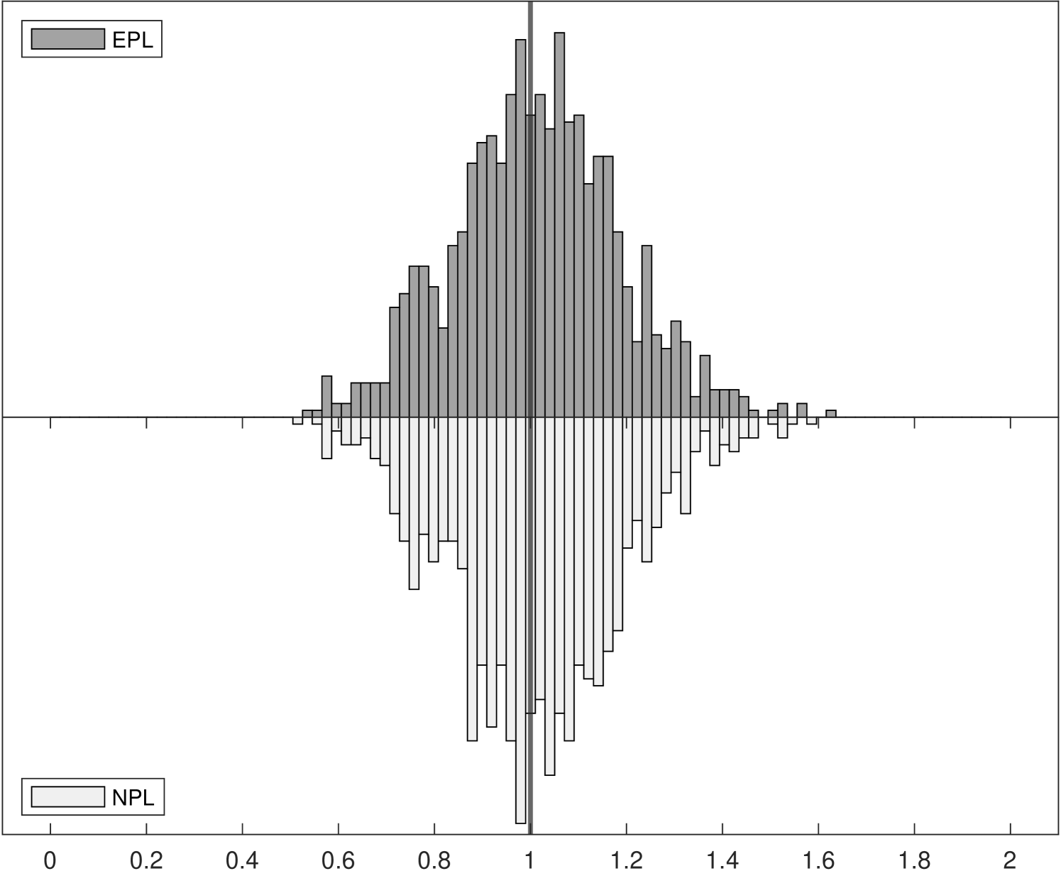
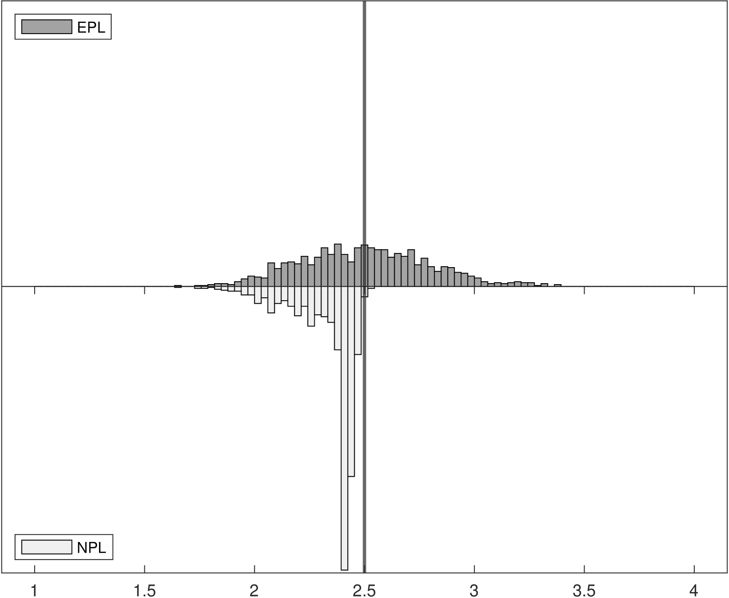
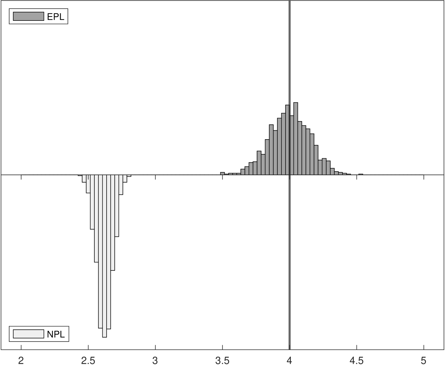
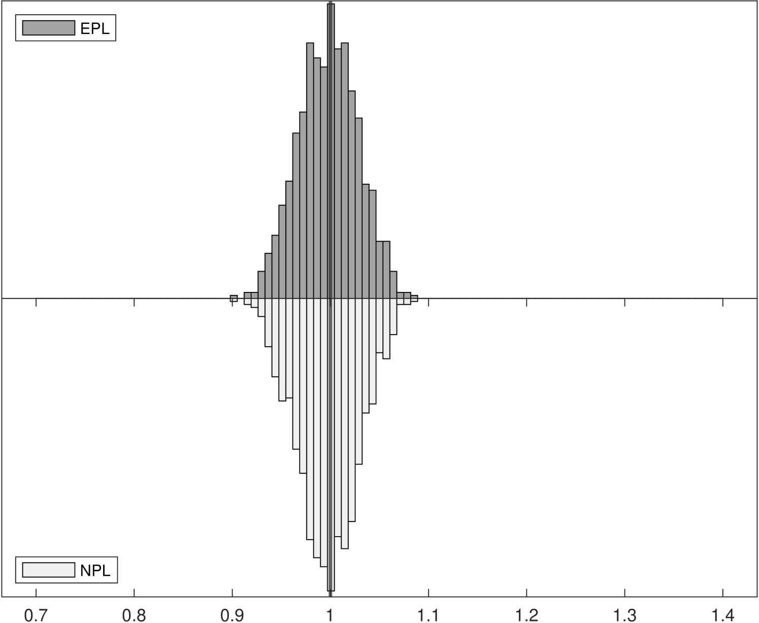
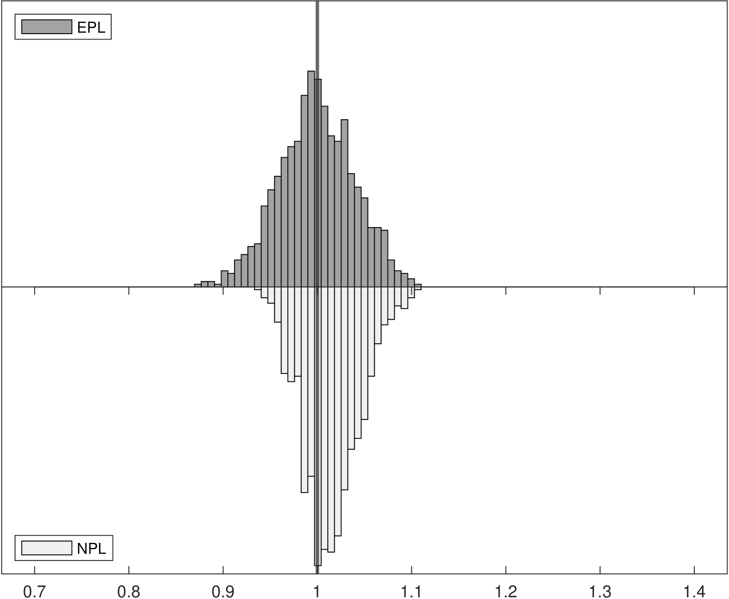
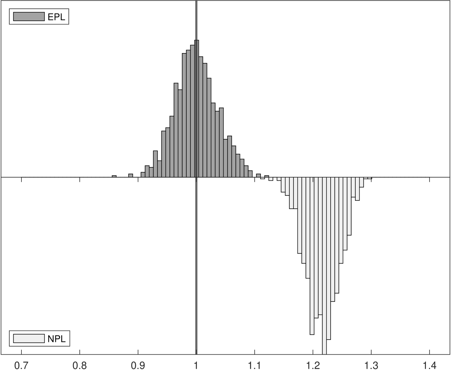
Figure 1 shows the Monte Carlo distributions of two key parameter estimates in the model: , the competitive effect, and , the entry cost. Each panel compares two histograms: the histogram above in dark gray corresponds to -EPL and the histogram below in light gray is for -NPL. These histograms are based on data for 1,000 replications of each experiment with 6,400 observations.
The left panels of Figure 1 show the distributions of , which is related to the strength of competition in the market and is closely related with the spectral radius of the NPL operator (while the spectral radius of the EPL operator is always zero). Indeed, we can see that as the competitive effect becomes large the distribution of -NPL estimates is truncated at around in Experiment 2. It remains concentrated around in Experiment 3 even though the value used in the data generating process was . Yet for all experiments the distributions of -EPL estimates are centered around the true values.
Although the true entry cost parameter is fixed at in all three experiments, the distribution of estimates can be affected when we vary the competitive effect from to . In the right panels of Figure 1, the truncation from above of in the -NPL distribution induces truncation from below in , as lower estimated values of competition result in higher estimated entry costs, leading to distortion of both distributions and to parameter estimates that would lead a policy-maker to possibly very different economic implications. In Experiment 3, although the distribution of -NPL estimates again appear to be normally distributed for both parameters, they are biased and are not centered around the true values.
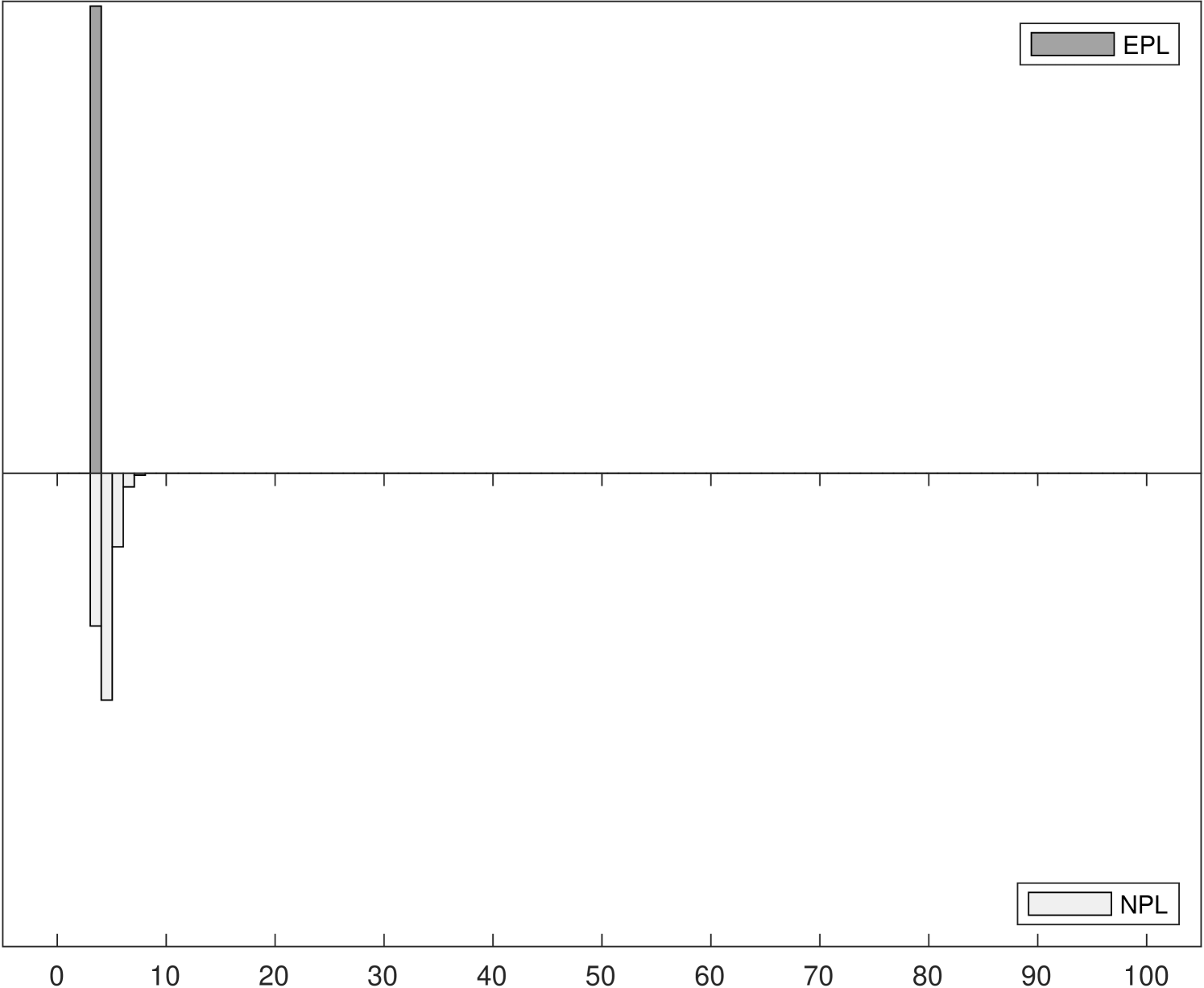
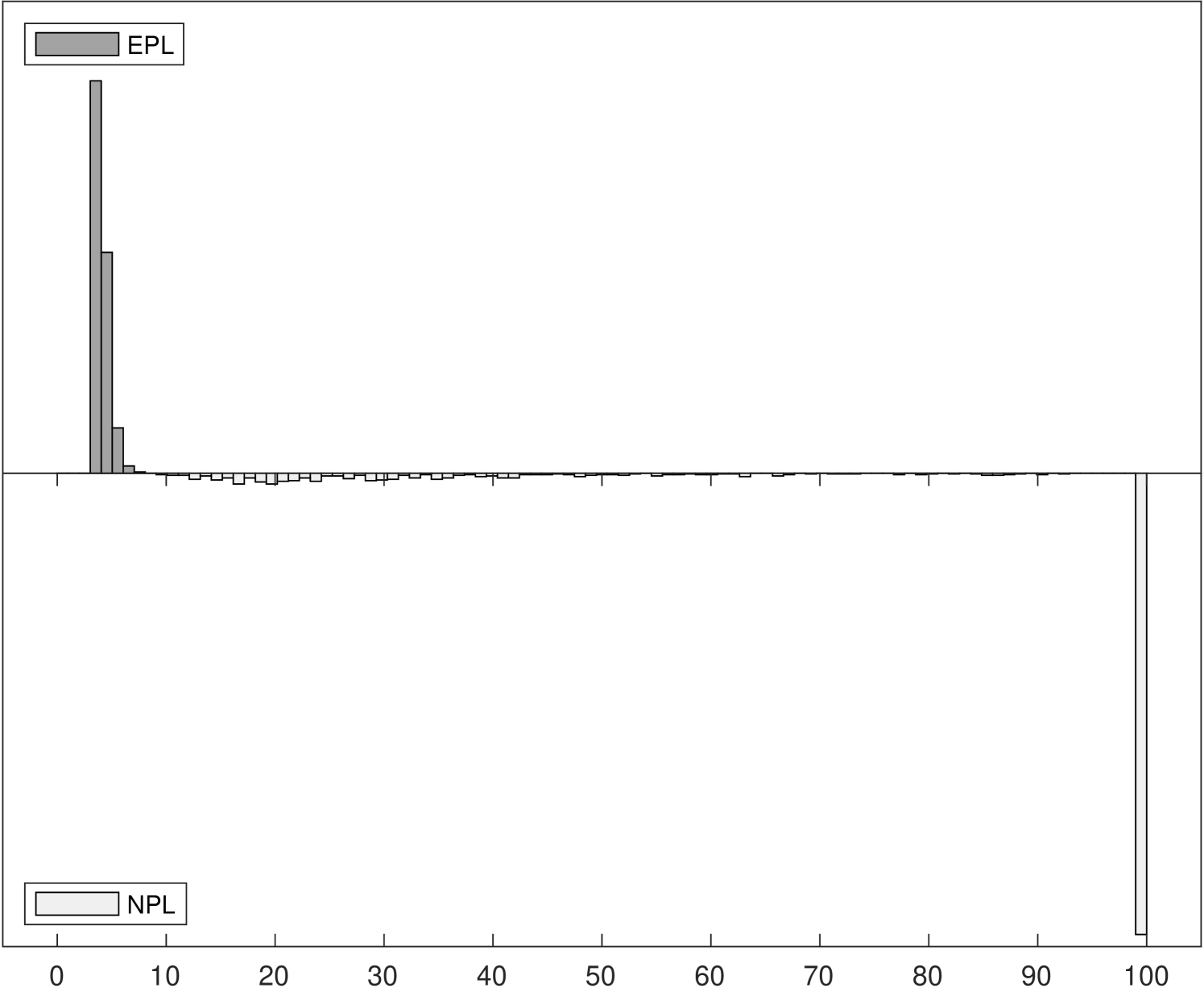
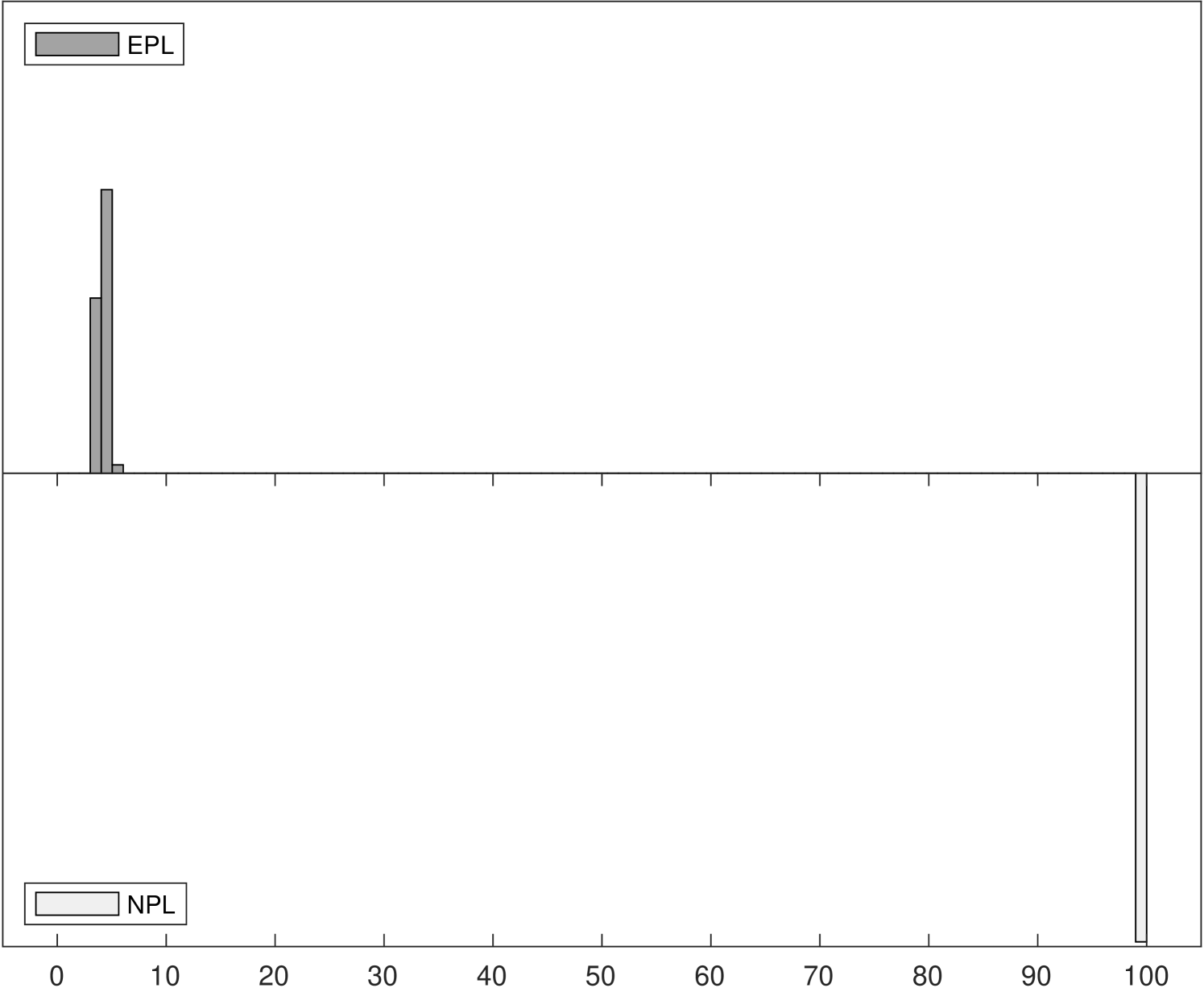
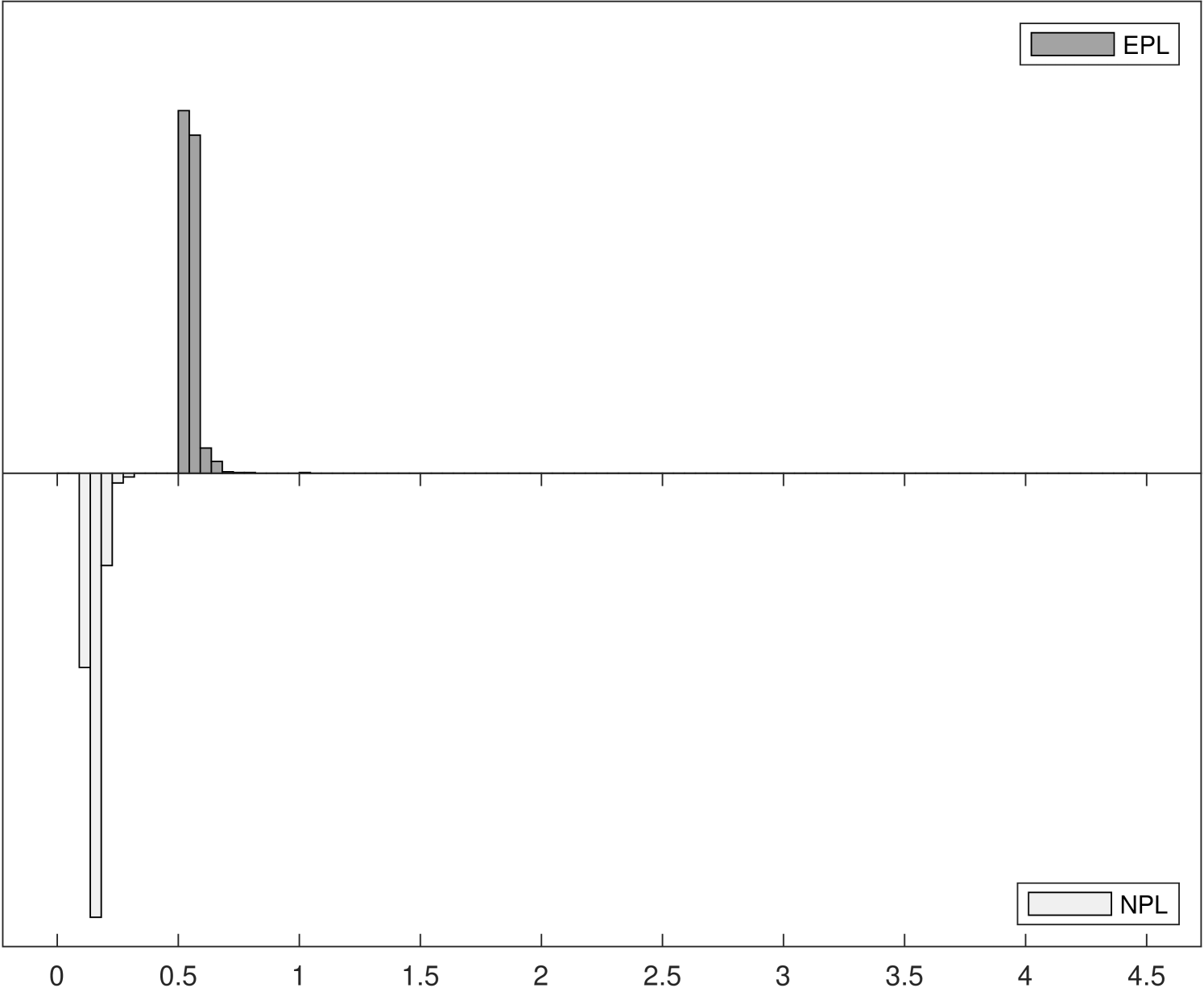
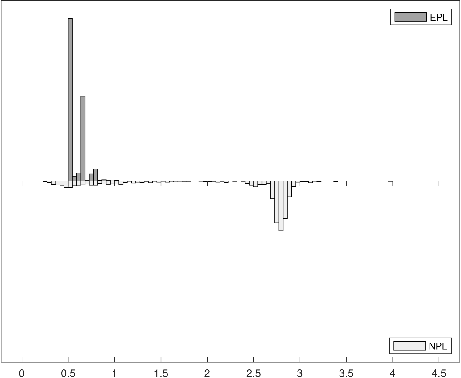
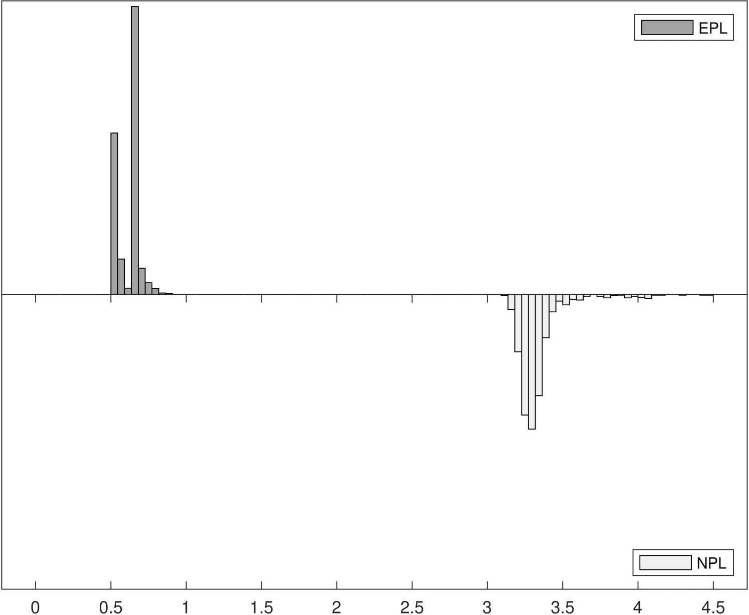
Figure 2 shows the distributions of iteration counts and computational times for -EPL and -NPL across the three experiments.222222Computational times are reported using Matlab R2020b on a 2019 Mac Pro with a 3.5 GHz 8-Core Intel Xeon W processor. The histograms in the left panels show the distribution of iteration counts required to achieve convergence for both estimators. Recall that the maximum number of iterations allowed was 100. -EPL requires fewer iterations for all experiments, especially for Experiments 2 and 3 where -NPL sometimes fails to converge in Experiment 2 and always fails to converge in Experiment 3. -EPL converged for all replications in all experiments.
The histograms in the right panels of Figure 2 show the distribution of total computational time, in seconds, across the 1000 replications. In Experiment 1, where -NPL is stable, -NPL is faster even though it requires more iterations on average. In other words, each -EPL iteration is more expensive on average, but fewer are required. This is in line with the analysis in Section 3.3. However, in Experiments 2 and 3 the computational times for -NPL increase as it requires more iterations, eventually overtaking the time required for -EPL yet still frequently (Experiment 2) or always (Experiment 3) failing to converge.
Summary statistics for all parameter estimates and all three experiments can be found in Tables 1–6. Each table reports summary statistics for 1-, 2-, 3-, and -NPL and 1-, 2-, 3-, and -EPL over the 1000 Monte Carlo replications for or . The upper two panels report the mean bias and mean square error (MSE) for each parameter and each sequential estimator. The next panel reports summary statistics for the number of iterations completed until either convergence or failure at 100 iterations. This includes the median, maximum, and inter-quartile range (IQR) of iteration counts across the replications as well as the number of replications for which -NPL failed to converge. Finally, the bottom panel reports the computational times for each estimator including the mean and median total time (for all completed iterations) across the 1000 replications and the median time per iteration.
| Bias | True | 1-NPL | 1-EPL | 2-NPL | 2-EPL | 3-NPL | 3-EPL | -NPL | -EPL |
|---|---|---|---|---|---|---|---|---|---|
| -1.9 | -0.018 | 0.007 | 0.008 | 0.004 | 0.002 | 0.004 | 0.004 | 0.005 | |
| -1.8 | -0.016 | 0.007 | 0.007 | 0.003 | 0.002 | 0.004 | 0.003 | 0.004 | |
| -1.7 | -0.018 | 0.003 | 0.003 | -0.001 | -0.002 | 0.000 | -0.001 | 0.000 | |
| -1.6 | -0.015 | 0.003 | 0.004 | 0.000 | -0.001 | 0.001 | 0.000 | 0.001 | |
| -1.5 | -0.013 | 0.003 | 0.004 | 0.000 | -0.001 | 0.000 | 0.000 | 0.000 | |
| 1.0 | -0.018 | 0.010 | 0.010 | 0.013 | 0.014 | 0.015 | 0.014 | 0.015 | |
| 1.0 | -0.068 | 0.034 | 0.034 | 0.038 | 0.040 | 0.044 | 0.041 | 0.044 | |
| 1.0 | -0.000 | 0.002 | 0.003 | -0.001 | -0.002 | -0.001 | -0.001 | -0.001 | |
| MSE | True | 1-NPL | 1-EPL | 2-NPL | 2-EPL | 3-NPL | 3-EPL | -NPL | -EPL |
| -1.9 | 0.012 | 0.013 | 0.013 | 0.013 | 0.013 | 0.013 | 0.013 | 0.013 | |
| -1.8 | 0.012 | 0.012 | 0.012 | 0.012 | 0.012 | 0.012 | 0.012 | 0.012 | |
| -1.7 | 0.011 | 0.012 | 0.012 | 0.012 | 0.012 | 0.012 | 0.012 | 0.012 | |
| -1.6 | 0.010 | 0.011 | 0.011 | 0.011 | 0.011 | 0.011 | 0.011 | 0.011 | |
| -1.5 | 0.009 | 0.010 | 0.010 | 0.009 | 0.009 | 0.009 | 0.009 | 0.009 | |
| 1.0 | 0.010 | 0.013 | 0.013 | 0.013 | 0.014 | 0.014 | 0.014 | 0.014 | |
| 1.0 | 0.091 | 0.123 | 0.123 | 0.128 | 0.128 | 0.130 | 0.129 | 0.131 | |
| 1.0 | 0.004 | 0.004 | 0.004 | 0.004 | 0.004 | 0.004 | 0.004 | 0.004 | |
| Iterations | 1-NPL | 1-EPL | 2-NPL | 2-EPL | 3-NPL | 3-EPL | -NPL | -EPL | |
| Median | 1 | 1 | 2 | 2 | 3 | 3 | 5 | 4 | |
| Max | 1 | 1 | 2 | 2 | 3 | 3 | 100 | 7 | |
| IQR | 2 | 0 | |||||||
| Non-Conv. | 0.1% | 0% | |||||||
| Time (sec.) | 1-NPL | 1-EPL | 2-NPL | 2-EPL | 3-NPL | 3-EPL | -NPL | -EPL | |
| Total | 17.88 | 118.42 | 31.33 | 234.82 | 44.35 | 350.07 | 76.55 | 481.70 | |
| Mean | 0.02 | 0.12 | 0.03 | 0.23 | 0.04 | 0.35 | 0.08 | 0.48 | |
| Median | 0.02 | 0.12 | 0.03 | 0.23 | 0.04 | 0.35 | 0.07 | 0.46 | |
| Med./Iter. | 0.018 | 0.118 | 0.016 | 0.117 | 0.015 | 0.116 | 0.014 | 0.116 | |
| Bias | True | 1-NPL | 1-EPL | 2-NPL | 2-EPL | 3-NPL | 3-EPL | -NPL | -EPL |
|---|---|---|---|---|---|---|---|---|---|
| -1.9 | -0.018 | 0.003 | 0.003 | 0.000 | -0.001 | 0.000 | 0.000 | 0.000 | |
| -1.8 | -0.017 | 0.002 | 0.002 | -0.001 | -0.002 | -0.001 | -0.001 | -0.001 | |
| -1.7 | -0.016 | 0.001 | 0.001 | -0.002 | -0.002 | -0.001 | -0.001 | -0.001 | |
| -1.6 | -0.013 | 0.003 | 0.003 | -0.000 | -0.001 | -0.000 | -0.000 | -0.000 | |
| -1.5 | -0.012 | 0.001 | 0.001 | -0.002 | -0.003 | -0.002 | -0.002 | -0.002 | |
| 1.0 | -0.022 | 0.003 | 0.003 | 0.004 | 0.005 | 0.005 | 0.005 | 0.005 | |
| 1.0 | -0.078 | 0.010 | 0.010 | 0.011 | 0.012 | 0.013 | 0.013 | 0.013 | |
| 1.0 | -0.001 | 0.000 | 0.001 | -0.002 | -0.003 | -0.002 | -0.002 | -0.002 | |
| MSE | True | 1-NPL | 1-EPL | 2-NPL | 2-EPL | 3-NPL | 3-EPL | -NPL | -EPL |
| -1.9 | 0.003 | 0.003 | 0.003 | 0.003 | 0.003 | 0.003 | 0.003 | 0.003 | |
| -1.8 | 0.003 | 0.003 | 0.003 | 0.003 | 0.003 | 0.003 | 0.003 | 0.003 | |
| -1.7 | 0.003 | 0.003 | 0.003 | 0.003 | 0.003 | 0.003 | 0.003 | 0.003 | |
| -1.6 | 0.003 | 0.003 | 0.003 | 0.003 | 0.003 | 0.003 | 0.003 | 0.003 | |
| -1.5 | 0.003 | 0.003 | 0.003 | 0.002 | 0.003 | 0.002 | 0.003 | 0.002 | |
| 1.0 | 0.003 | 0.003 | 0.003 | 0.003 | 0.003 | 0.003 | 0.003 | 0.003 | |
| 1.0 | 0.027 | 0.030 | 0.030 | 0.030 | 0.030 | 0.030 | 0.031 | 0.030 | |
| 1.0 | 0.001 | 0.001 | 0.001 | 0.001 | 0.001 | 0.001 | 0.001 | 0.001 | |
| Iterations | 1-NPL | 1-EPL | 2-NPL | 2-EPL | 3-NPL | 3-EPL | -NPL | -EPL | |
| Median | 1 | 1 | 2 | 2 | 3 | 3 | 5 | 4 | |
| Max | 1 | 1 | 2 | 2 | 3 | 3 | 8 | 4 | |
| IQR | 1 | 0 | |||||||
| Non-Conv. | 0% | 0% | |||||||
| Time (sec.) | 1-NPL | 1-EPL | 2-NPL | 2-EPL | 3-NPL | 3-EPL | -NPL | -EPL | |
| Total | 43.91 | 148.28 | 75.66 | 284.75 | 105.45 | 416.53 | 154.35 | 548.53 | |
| Mean | 0.04 | 0.15 | 0.08 | 0.28 | 0.11 | 0.42 | 0.15 | 0.55 | |
| Median | 0.04 | 0.15 | 0.07 | 0.28 | 0.10 | 0.41 | 0.15 | 0.55 | |
| Med./Iter. | 0.043 | 0.147 | 0.037 | 0.141 | 0.034 | 0.138 | 0.031 | 0.136 | |
For Experiment 1, both the -NPL and -EPL estimators perform equally well with low bias, as can be seen in Tables 1 and 2. The parameter with the most finite-sample variation is also the main parameter of interest in our study: Note that in this model, in order to obtain estimates with performance similar to the converged estimates it would suffice to stop at 3 iterations with either estimator. Typically, both -NPL and -EPL converge in 4 to 5 iterations. However, even in this specification where -NPL performs well, in one case out of 1000, -NPL fails to converge in 100 iterations or less while -EPL always converges in at most 7 iterations. In terms of computational time, in this model due to the computational complexity, in the median experiment one iteration of -EPL is more expensive (0.3 seconds) than one iteration of -NPL (0.045 seconds). Because roughly the same number of iterations are required in this model, the overall times for -EPL are also longer than for -NPL. However, even with the increased complexity each replication of -EPL takes only around 1.3 seconds to estimate, so it remains quite feasible.
| Bias | True | 1-NPL | 1-EPL | 2-NPL | 2-EPL | 3-NPL | 3-EPL | -NPL | -EPL |
|---|---|---|---|---|---|---|---|---|---|
| -1.9 | -0.005 | -0.002 | -0.002 | -0.001 | -0.008 | -0.003 | 0.006 | -0.003 | |
| -1.8 | -0.002 | -0.004 | -0.005 | -0.002 | -0.005 | -0.004 | 0.010 | -0.004 | |
| -1.7 | 0.003 | -0.006 | -0.007 | -0.001 | -0.000 | -0.004 | 0.014 | -0.004 | |
| -1.6 | 0.007 | -0.008 | -0.009 | -0.002 | 0.002 | -0.006 | 0.016 | -0.006 | |
| -1.5 | 0.011 | -0.009 | -0.010 | -0.002 | 0.005 | -0.007 | 0.017 | -0.008 | |
| 1.0 | 0.012 | 0.007 | 0.006 | -0.006 | -0.006 | 0.007 | -0.063 | 0.008 | |
| 1.0 | 0.056 | 0.024 | 0.017 | -0.026 | -0.027 | 0.025 | -0.261 | 0.030 | |
| 1.0 | -0.002 | -0.001 | -0.001 | 0.004 | 0.001 | -0.002 | 0.027 | -0.003 | |
| MSE | True | 1-NPL | 1-EPL | 2-NPL | 2-EPL | 3-NPL | 3-EPL | -NPL | -EPL |
| -1.9 | 0.016 | 0.015 | 0.015 | 0.015 | 0.016 | 0.015 | 0.014 | 0.015 | |
| -1.8 | 0.016 | 0.015 | 0.015 | 0.014 | 0.015 | 0.015 | 0.013 | 0.015 | |
| -1.7 | 0.016 | 0.015 | 0.015 | 0.014 | 0.015 | 0.015 | 0.013 | 0.015 | |
| -1.6 | 0.016 | 0.015 | 0.015 | 0.014 | 0.015 | 0.015 | 0.012 | 0.015 | |
| -1.5 | 0.018 | 0.017 | 0.017 | 0.016 | 0.016 | 0.016 | 0.013 | 0.017 | |
| 1.0 | 0.029 | 0.023 | 0.023 | 0.019 | 0.018 | 0.021 | 0.010 | 0.021 | |
| 1.0 | 0.468 | 0.365 | 0.359 | 0.310 | 0.282 | 0.327 | 0.162 | 0.335 | |
| 1.0 | 0.008 | 0.007 | 0.007 | 0.006 | 0.006 | 0.006 | 0.004 | 0.006 | |
| Iterations | 1-NPL | 1-EPL | 2-NPL | 2-EPL | 3-NPL | 3-EPL | -NPL | -EPL | |
| Median | 1 | 1 | 2 | 2 | 3 | 3 | 100 | 5 | |
| Max | 1 | 1 | 2 | 2 | 3 | 3 | 100 | 30 | |
| IQR | 75.5 | 2 | |||||||
| Non-Conv. | 61.2% | 0% | |||||||
| Time (sec.) | 1-NPL | 1-EPL | 2-NPL | 2-EPL | 3-NPL | 3-EPL | -NPL | -EPL | |
| Total | 18.26 | 120.53 | 32.92 | 239.61 | 47.60 | 358.72 | 1030.36 | 672.18 | |
| Mean | 0.02 | 0.12 | 0.03 | 0.24 | 0.05 | 0.36 | 1.03 | 0.67 | |
| Median | 0.02 | 0.12 | 0.03 | 0.24 | 0.05 | 0.36 | 1.44 | 0.60 | |
| Med./Iter. | 0.018 | 0.120 | 0.016 | 0.119 | 0.016 | 0.119 | 0.014 | 0.118 | |
| Bias | True | 1-NPL | 1-EPL | 2-NPL | 2-EPL | 3-NPL | 3-EPL | -NPL | -EPL |
|---|---|---|---|---|---|---|---|---|---|
| -1.9 | -0.002 | -0.000 | -0.001 | -0.002 | -0.005 | -0.002 | 0.006 | -0.002 | |
| -1.8 | 0.002 | -0.002 | -0.003 | -0.002 | -0.002 | -0.002 | 0.008 | -0.002 | |
| -1.7 | 0.006 | -0.004 | -0.005 | -0.002 | 0.000 | -0.003 | 0.009 | -0.003 | |
| -1.6 | 0.012 | -0.004 | -0.005 | -0.001 | 0.004 | -0.002 | 0.010 | -0.002 | |
| -1.5 | 0.019 | -0.004 | -0.005 | -0.001 | 0.007 | -0.003 | 0.008 | -0.003 | |
| 1.0 | -0.001 | 0.001 | 0.001 | -0.003 | -0.005 | 0.001 | -0.040 | 0.001 | |
| 1.0 | 0.003 | 0.002 | -0.003 | -0.013 | -0.018 | 0.001 | -0.163 | 0.002 | |
| 1.0 | 0.003 | -0.000 | 0.000 | 0.000 | 0.000 | -0.001 | 0.015 | -0.001 | |
| MSE | True | 1-NPL | 1-EPL | 2-NPL | 2-EPL | 3-NPL | 3-EPL | -NPL | -EPL |
| -1.9 | 0.004 | 0.004 | 0.004 | 0.004 | 0.004 | 0.004 | 0.004 | 0.004 | |
| -1.8 | 0.004 | 0.004 | 0.004 | 0.004 | 0.004 | 0.004 | 0.003 | 0.004 | |
| -1.7 | 0.004 | 0.004 | 0.004 | 0.004 | 0.004 | 0.004 | 0.003 | 0.004 | |
| -1.6 | 0.004 | 0.004 | 0.004 | 0.004 | 0.004 | 0.004 | 0.003 | 0.004 | |
| -1.5 | 0.004 | 0.004 | 0.004 | 0.004 | 0.004 | 0.004 | 0.004 | 0.004 | |
| 1.0 | 0.007 | 0.006 | 0.006 | 0.005 | 0.005 | 0.006 | 0.003 | 0.006 | |
| 1.0 | 0.109 | 0.096 | 0.095 | 0.085 | 0.084 | 0.087 | 0.048 | 0.088 | |
| 1.0 | 0.002 | 0.002 | 0.002 | 0.002 | 0.002 | 0.002 | 0.001 | 0.002 | |
| Iterations | 1-NPL | 1-EPL | 2-NPL | 2-EPL | 3-NPL | 3-EPL | -NPL | -EPL | |
| Median | 1 | 1 | 2 | 2 | 3 | 3 | 100 | 4 | |
| Max | 1 | 1 | 2 | 2 | 3 | 3 | 100 | 8 | |
| IQR | 52 | 1 | |||||||
| Non-Conv. | 68.9% | 0% | |||||||
| Time (sec.) | 1-NPL | 1-EPL | 2-NPL | 2-EPL | 3-NPL | 3-EPL | -NPL | -EPL | |
| Total | 35.34 | 135.62 | 64.32 | 266.26 | 92.87 | 395.24 | 2186.69 | 586.21 | |
| Mean | 0.04 | 0.14 | 0.06 | 0.27 | 0.09 | 0.40 | 2.19 | 0.59 | |
| Median | 0.03 | 0.13 | 0.06 | 0.26 | 0.09 | 0.39 | 2.75 | 0.53 | |
| Med./Iter. | 0.034 | 0.135 | 0.032 | 0.132 | 0.031 | 0.131 | 0.028 | 0.130 | |
In Experiment 2, we begin to see a divergence between the two methods. As reported by Aguirregabiria and Marcoux (2021), the spectral radius of the population NPL operator is slightly larger than one for this specification. In finite random samples, sometimes the sample counterpart is stable and sometimes it is unstable. This leads to the situation illustrated by Table 3, where -NPL fails to converge in 612 of 1000 replications. -EPL, on the other hand, is stable and converges for all 1000 replications. Importantly, the 1-NPL estimator obtained without further iterations is always consistent. However, there is substantial bias in the -NPL estimates. In an apparent contradiction, the MSE for is actually lower for -NPL than for -EPL. This pattern of larger bias and lower MSE is seen again with the large sample size in Table 4, however it can be understood simply by recalling the histogram of the estimates (panel (b) of Figure 1). The -NPL sampling distribution appears to be truncated near 2.4, which perhaps not coincidentally is near the value where the spectral radius exceeds one (Aguirregabiria and Marcoux (2021)). Since this happens to be close to the true parameter value, the MSE is artificially low. However, the sampling distribution is neither normally distributed nor centered at the true value. A K-S test for normality of the -NPL estimates has a -value equal to zero up to three decimal places, while for -EPL the -value is 0.622.
In Experiment 2 we also see a reversal of the order of computational times: the non-convergent -NPL cases require more iterations and more time per iteration, while -EPL always converges in 8 or fewer iterations. Thus, in thinking about the trade-off between robustness and computational time we should also consider convergence. A non-convergent estimator may take longer and yield worse results in the end. -EPL does require more time per iteration in this model, but it is more robust to the strength of competition in the model.
| Bias | True | 1-NPL | 1-EPL | 2-NPL | 2-EPL | 3-NPL | 3-EPL | -NPL | -EPL |
|---|---|---|---|---|---|---|---|---|---|
| -1.9 | -0.100 | 0.010 | 0.008 | -0.002 | -0.095 | 0.002 | 0.012 | 0.002 | |
| -1.8 | -0.088 | 0.000 | -0.001 | -0.000 | -0.074 | 0.002 | 0.031 | 0.002 | |
| -1.7 | -0.066 | -0.010 | -0.011 | 0.000 | -0.040 | 0.001 | 0.062 | 0.002 | |
| -1.6 | -0.016 | -0.016 | -0.017 | 0.004 | 0.026 | 0.002 | 0.131 | 0.002 | |
| -1.5 | 0.050 | -0.007 | -0.005 | 0.009 | 0.156 | 0.000 | 0.211 | -0.000 | |
| 1.0 | 0.042 | -0.005 | -0.019 | -0.009 | -0.108 | 0.001 | -0.244 | 0.001 | |
| 1.0 | 0.198 | -0.067 | -0.147 | -0.055 | -0.640 | 0.004 | -1.382 | 0.008 | |
| 1.0 | -0.009 | 0.025 | 0.031 | 0.010 | 0.073 | 0.001 | 0.218 | -0.000 | |
| MSE | True | 1-NPL | 1-EPL | 2-NPL | 2-EPL | 3-NPL | 3-EPL | -NPL | -EPL |
| -1.9 | 0.038 | 0.022 | 0.022 | 0.023 | 0.032 | 0.023 | 0.019 | 0.023 | |
| -1.8 | 0.034 | 0.020 | 0.020 | 0.021 | 0.026 | 0.021 | 0.018 | 0.021 | |
| -1.7 | 0.030 | 0.020 | 0.019 | 0.019 | 0.021 | 0.020 | 0.020 | 0.020 | |
| -1.6 | 0.028 | 0.019 | 0.019 | 0.019 | 0.019 | 0.019 | 0.032 | 0.019 | |
| -1.5 | 0.039 | 0.022 | 0.021 | 0.019 | 0.041 | 0.019 | 0.057 | 0.019 | |
| 1.0 | 0.022 | 0.006 | 0.006 | 0.004 | 0.015 | 0.004 | 0.061 | 0.004 | |
| 1.0 | 0.602 | 0.126 | 0.131 | 0.090 | 0.456 | 0.086 | 1.924 | 0.086 | |
| 1.0 | 0.022 | 0.007 | 0.007 | 0.005 | 0.009 | 0.005 | 0.051 | 0.005 | |
| Iterations | 1-NPL | 1-EPL | 2-NPL | 2-EPL | 3-NPL | 3-EPL | -NPL | -EPL | |
| Median | 1 | 1 | 2 | 2 | 3 | 3 | 100 | 5 | |
| Max | 1 | 1 | 2 | 2 | 3 | 3 | 100 | 9 | |
| IQR | 0 | 1 | |||||||
| Non-Conv. | 100% | 0% | |||||||
| Time (sec.) | 1-NPL | 1-EPL | 2-NPL | 2-EPL | 3-NPL | 3-EPL | -NPL | -EPL | |
| Total | 18.64 | 125.88 | 33.88 | 246.85 | 48.96 | 367.25 | 1512.68 | 654.05 | |
| Mean | 0.02 | 0.13 | 0.03 | 0.25 | 0.05 | 0.37 | 1.51 | 0.65 | |
| Median | 0.02 | 0.12 | 0.03 | 0.24 | 0.05 | 0.36 | 1.48 | 0.62 | |
| Med./Iter. | 0.018 | 0.124 | 0.017 | 0.122 | 0.016 | 0.120 | 0.015 | 0.119 | |
| Bias | True | 1-NPL | 1-EPL | 2-NPL | 2-EPL | 3-NPL | 3-EPL | -NPL | -EPL |
|---|---|---|---|---|---|---|---|---|---|
| -1.9 | -0.098 | 0.008 | 0.007 | 0.000 | -0.098 | 0.000 | 0.013 | 0.000 | |
| -1.8 | -0.086 | -0.003 | -0.003 | 0.000 | -0.078 | 0.000 | 0.031 | 0.000 | |
| -1.7 | -0.063 | -0.015 | -0.016 | 0.001 | -0.045 | -0.001 | 0.062 | -0.001 | |
| -1.6 | -0.013 | -0.024 | -0.025 | 0.004 | 0.017 | 0.000 | 0.130 | 0.000 | |
| -1.5 | 0.057 | -0.025 | -0.023 | 0.009 | 0.139 | 0.000 | 0.207 | 0.000 | |
| 1.0 | 0.034 | 0.011 | -0.003 | -0.010 | -0.096 | 0.000 | -0.243 | 0.000 | |
| 1.0 | 0.155 | 0.024 | -0.054 | -0.057 | -0.570 | -0.001 | -1.377 | 0.000 | |
| 1.0 | 0.001 | 0.011 | 0.016 | 0.008 | 0.060 | 0.000 | 0.216 | 0.000 | |
| MSE | True | 1-NPL | 1-EPL | 2-NPL | 2-EPL | 3-NPL | 3-EPL | -NPL | -EPL |
| -1.9 | 0.016 | 0.005 | 0.005 | 0.005 | 0.015 | 0.005 | 0.005 | 0.005 | |
| -1.8 | 0.014 | 0.005 | 0.005 | 0.005 | 0.011 | 0.005 | 0.005 | 0.005 | |
| -1.7 | 0.011 | 0.005 | 0.005 | 0.005 | 0.007 | 0.005 | 0.008 | 0.005 | |
| -1.6 | 0.007 | 0.006 | 0.006 | 0.005 | 0.005 | 0.005 | 0.020 | 0.005 | |
| -1.5 | 0.012 | 0.006 | 0.006 | 0.005 | 0.024 | 0.005 | 0.046 | 0.005 | |
| 1.0 | 0.006 | 0.002 | 0.001 | 0.001 | 0.010 | 0.001 | 0.060 | 0.001 | |
| 1.0 | 0.167 | 0.037 | 0.034 | 0.023 | 0.335 | 0.023 | 1.900 | 0.023 | |
| 1.0 | 0.005 | 0.002 | 0.002 | 0.001 | 0.004 | 0.001 | 0.048 | 0.001 | |
| Iterations | 1-NPL | 1-EPL | 2-NPL | 2-EPL | 3-NPL | 3-EPL | -NPL | -EPL | |
| Median | 1 | 1 | 2 | 2 | 3 | 3 | 100 | 5 | |
| Max | 1 | 1 | 2 | 2 | 3 | 3 | 100 | 6 | |
| IQR | 0 | 1 | |||||||
| Non-Conv. | 100% | 0% | |||||||
| Time (sec.) | 1-NPL | 1-EPL | 2-NPL | 2-EPL | 3-NPL | 3-EPL | -NPL | -EPL | |
| Total | 40.48 | 145.93 | 75.22 | 278.93 | 108.36 | 410.64 | 3332.77 | 620.36 | |
| Mean | 0.04 | 0.15 | 0.08 | 0.28 | 0.11 | 0.41 | 3.33 | 0.62 | |
| Median | 0.04 | 0.14 | 0.07 | 0.28 | 0.11 | 0.41 | 3.30 | 0.65 | |
| Med./Iter. | 0.039 | 0.145 | 0.037 | 0.138 | 0.035 | 0.136 | 0.033 | 0.133 | |
Turning to Experiment 3, we increase the effect of competition even further to where , well beyond the point where -NPL becomes unstable. In this case, both with small samples and large samples, -NPL fails to converge in all 1000 replications but -EPL converges in all 1000 replications. In these cases, the bias in -NPL estimates is larger and in this case and so is the MSE, since the value of is farther from the point of truncation than in Experiment 2. The -NPL estimator systematically underestimates the competitive effect and overestimates the entry cost .
Overall, across the three experiments the performance of -EPL is stable and of similar quality despite the increasing competitive effect. This result agrees with our theoretical analysis showing that -EPL is stable, convergent, and efficient.
Finally, we note that with the -EPL estimator there is very little performance improvement after the first three iterations. The performance of -EPL is achieved already, up to two decimal places, by 3-EPL. Thus, for this model one can reduce the computational time required while retaining efficiency and robustness by carrying out only a few iterations of -EPL.
5 Application to U.S. Wholesale Club Competition
The U.S. wholesale club store industry is a retail segment that offers members a wide range of merchandise at discounted prices. The industry is dominated by three major players: Sam’s Club, Costco, and BJ’s Wholesale Club. These companies operate as membership-based clubs, with a focus on bulk purchasing and high-volume sales.
The modern wholesale club store industry emerged in the 1970s with the founding of Price Club in San Diego, California. Price Club was a pioneer in the industry, offering its members deep discounts on products, including groceries, electronics, and household goods. In 1983, Costco was founded in Seattle, Washington, and quickly became a major player in the industry. Sam’s Club, a subsidiary of Walmart, was also founded in 1983. BJ’s Wholesale Club was founded in 1984 in Massachusetts. In 1993, Price Club merged with Costco and adopted the Costco name (Costco Wholesale Corporation (2023)).
Today, the wholesale club store industry is a major force in retail, with the three main players generating over $260 billion in annual revenue, according to data from their 2021 annual reports. Costco is the largest company in the industry, with over 800 stores worldwide and annual revenue of over $190 billion (Costco Wholesale Corporation (2021)). Sam’s Club is the second-largest, with around 600 stores and annual revenue of over $60 billion (Walmart Inc. (2021)). BJ’s Wholesale Club is the smallest of the three, with over 200 stores and annual revenue of over $16 billion (BJ’s Wholesale Club Holdings, Inc. (2022)).
Although we focus on Costco, Sam’s Club, and BJ’s, which are by far the largest firms in the industry, there are other smaller players. An example is DirectBuy, which was the 4th largest firm (by total markets served) in our sample. While it was a significant player in the home furnishings and home improvement space, it was not a direct competitor of Costco, Sam’s Club, and BJ’s and was significantly smaller. DirectBuy faced financial difficulties and filed for bankruptcy in 2018 (Engel (2016)).
5.1 Data
Our data come from the Data Axle Business Database which contains information on businesses across the United States. The company uses a variety of sources to gather information on businesses, including public records, government filings, and proprietary data sources. Our data begins in 2009 and ends in 2021. From this database we first extract records for each Sam’s Club, Costco, and BJ’s location. We augment this with ZIP code level population data obtained from NHGIS (Manson et al. (2022)). We then aggregate to county-level markets using the 2021 ZIP code to county crosswalk files provided by the U.S. Department of Housing and Urban Development (HUD). We consider all counties in the 50 states of the United States and the District of Columbia that have between 20,000 and 600,000 residents. This serves to exclude very small counties that would clearly not be considered for entry as well as some very large, atypical markets.
Overall, our final sample consists of counties observed over years.232323Although we have 13 years of data, we require lagged actions to construct the incumbency status state variable. As a result, the time dimension of our sample is reduced to . Among these markets, the average peak population during our sample was 104,841 with standard deviation 112,759.242424We compute peak population for a market as the maximum over the years in the sample. In the model, our market size variable, , is the logarithm of population discretized into 5 equal bins.252525We also tried 10 bins without any major substantive changes in the results. Table 7 presents summary statistics for our sample. On average, there are 0.348 active firms in each market with a standard deviation of 0.622. The autoregressive coefficient for the number of active firms is 0.987, indicating a strong positive correlation between the number of active firms in the current period and the previous period.262626This refers to the estimated autoregressive coefficient in an AR(1) regression of the number of current active firms on the number of active firms in previous period. The average number of entrants is 0.010, while the average number of exits is 0.006. Excess turnover, defined as (#entrants + #exits) - |#entrants - #exits|, is effectively zero. The correlation between entries and exits is -0.007. The probability of being active is highest for Sam’s Club at 0.201, followed by Costco at 0.093 and BJ’s at 0.054. The distribution of market size is such that there are relatively more small-to-medium size markets markets and relatively fewer large markets.
| Statistic | Value |
|---|---|
| Average active firms | 0.348 |
| S.D. active firms | 0.622 |
| AR(1) for active firms | 0.987 |
| Average entrants | 0.010 |
| Average exits | 0.006 |
| Excess turnover | 0.000 |
| Correlation between entries and exits | -0.007 |
| Probability of being active | |
| Sam’s Club | 0.201 |
| Costco | 0.093 |
| BJ’s | 0.054 |
| Distribution of market size | |
| 0.332 | |
| 0.295 | |
| 0.179 | |
| 0.125 | |
| 0.069 | |
| Markets | 1,610 |
| Years | 12 |
| Observations (Markets Years) | 19,320 |
5.2 Model
Our model of wholesale club competition follows the dynamic oligopoly model with heterogeneous firms described in Example 1 and also used in our Monte Carlo experiments in Section 4. In our application the firms are denoted . In each market and time period , firms decide whether to operate in a market () or not (). The profit function has the following form for an active firm :
Here, is the fixed cost of operation for firm j, is the cost incurred by a new entrant, represents the effect of market size (the discretized logarithm of population, defined above), and captures the effect of competition. When firm is inactive, .
5.3 Structural Parameter Estimates
Using -EPL, we estimate the heterogeneous fixed costs , , and as well as the entry cost , the coefficient on market size , and the competitive effect parameters of the model.
Table 8 reports the point estimates from the observed sample along with standard errors and 95% confidence intervals estimated using 250 cross-sectional bootstrap replications. The estimates all have the expected sign and are all significantly different from zero at the 5% level. Fixed costs are lowest for Sam’s Club and highest for BJ’s. Firms are more profitable in larger markets and entry by competitors reduces profits. The entry cost is large relative to fixed costs, as expected.
| Parameter | Estimate | S.E. | 95% CI |
|---|---|---|---|
| -0.136 | (0.030) | [-0.196, -0.079] | |
| -0.130 | (0.031) | [-0.188, -0.073] | |
| -0.197 | (0.030) | [-0.255, -0.143] | |
| 0.106 | (0.009) | [0.090, 0.124] | |
| 0.137 | (0.030) | [0.087, 0.210] | |
| 8.855 | (0.163) | [8.559, 9.186] |
We note that for this application -NPL yields very similar results to -EPL. The estimated competitive effect is small, implying that -NPL is likely to be stable. However, we could not know this a priori (recall that in our Monte Carlo Experiments, the -NPL estimates of the competitive effect are biased towards zero). However, ex post, with the stable -EPL estimates in hand, we can understand the performance of -NPL this setting.
5.4 Counterfactual
The industry under investigation is characterized by a significant number of monopoly markets. In the latest year of our sample, 2021, we observed a mere 14 triopoly markets (less than 1% of our sample). Only 7% of the markets had a duopoly, with two firms present, while 20% of the markets were monopolies, where a single firm operated. Interestingly, 72% of counties in our sample had no wholesale club stores at all in 2021. Our counterfactual exercise aims to explore the reasons behind this relative scarcity of duopoly and triopoly markets. Are strong competitive effects or high costs responsible?
To address this question, we conduct a counterfactual simulation in which we entirely eliminate the competitive effect in the model, allowing firms to operate as independent agents without considering their competitors’ actions. If we observe a substantial increase in new entries, we may deduce that strong competition is deterring other firms from entering the market. Conversely, if we notice minimal change in entry behavior, it may suggest that competitive effects are insignificant, and costs are the primary factor driving firms’ entry decisions.
To investigate this, we take the estimated structural parameters from the observed sample, set , and compute the counterfactual equilibrium. We solve the nonlinear system of equilibrium equations using the estimated equilibrium as the starting value. Subsequently, we compare the results of simulations conducted under this counterfactual scenario to those obtained using the estimated model parameters. We perform this procedure for each bootstrap replication to calculate standard errors for the counterfactual quantities of interest. For every simulation, we employ the observed market configuration at the beginning of the sample in 2009 and simulate until the end of our sample period in 2021.
In Table 9, we present aggregate statistics from simulations using both the estimated and counterfactual parameters, where the competitive effect has been set to zero. The reported figures represent the estimated means and standard errors derived from simulated sample paths using the parameters from the 250 bootstrap replications. Before delving into the counterfactual analysis, it is worth noting that this can also serve as a test of the model’s fit. We observe that the average number of active firms, entries, and exits, as well as the distribution of the number of firms present, align reasonably well with the observed values from the data. Upon examining the counterfactual, we discover that removing the effect of competition does not significantly reduce the number of unserved markets (from 1164 to 1156). However, it does shift the distribution away from monopoly markets (from 341 down to 300) towards a higher prevalence of duopoly and triopoly markets (from 93 up to 118, and from 11 up to 34, respectively). These findings indicate that competition in this industry is relatively weak, and costs play a more significant role in determining entry behavior.
| Simulated | Counterfactual | ||||
| Observed | Mean | S.E. | Mean | S.E. | |
| Active Firms | 0.348 | 0.349 | (0.017) | 0.398 | (0.023) |
| Entries | 0.010 | 0.010 | (0.001) | 0.016 | (0.002) |
| Exits | 0.006 | 0.006 | (0.001) | 0.005 | (0.001) |
| Markets with | |||||
| 0 Firms | 1156 | 1164.665 | (27.805) | 1156.434 | (28.576) |
| 1 Firms | 321 | 340.598 | (24.424) | 300.371 | (22.650) |
| 2 Firms | 119 | 93.426 | (12.663) | 118.948 | (15.066) |
| 3 Firms | 14 | 11.311 | (4.940) | 34.247 | (9.687) |
Table 10 provides a more detailed breakdown of our simulations by firm and market size state . We estimate that, on average, Sam’s Club would enter approximately 3 additional small markets () and around 15 additional large markets (). Costco would enter, on average, 4 additional small markets and 28 large markets. BJ’s would enter, on average, 3 additional small markets and 27 large markets. Consequently, eliminating the competitive effect appears to have a proportionally much larger impact on BJ’s compared to Costco and Sam’s Club. This effect is also considerably more pronounced in larger markets than in smaller ones.
| Sam’s Club | Costco | BJ’s | ||||
| Mean | S.E. | Mean | S.E. | Mean | S.E. | |
| Estimated | ||||||
| 3.103 | (1.359) | 3.876 | (1.522) | 1.474 | (0.854) | |
| 19.384 | (4.153) | 12.480 | (3.134) | 5.739 | (2.011) | |
| 86.238 | (8.263) | 24.618 | (4.534) | 18.299 | (4.044) | |
| 127.656 | (11.218) | 54.597 | (7.234) | 29.962 | (5.098) | |
| 81.056 | (8.290) | 59.769 | (7.252) | 33.458 | (5.734) | |
| Counterfactual | ||||||
| 3.169 | (1.441) | 3.943 | (1.799) | 1.494 | (0.819) | |
| 19.892 | (4.232) | 12.889 | (3.268) | 5.784 | (2.208) | |
| 88.295 | (8.959) | 28.575 | (4.945) | 21.138 | (4.094) | |
| 135.488 | (11.393) | 70.326 | (8.880) | 41.387 | (7.177) | |
| 87.731 | (8.902) | 72.334 | (8.468) | 49.016 | (8.026) | |
Our analysis also incorporates average profit simulations using both the estimated parameters and the counterfactual parameters. To achieve this, for each simulation, we calculate for each firm and average it over each simulated sample path of states and choices.272727We simulate actions by sampling from the distribution defined by , so must be included to capture the contribution of to average profit. With Type 1 Extreme Value shocks, , where is the Euler-Mascheroni constant. We perform this separately for the simulations based on the model estimates and those under the counterfactual parameters. Comparing these two unit-less measures of profitability offers another perspective on our research question.
The results of this exercise are reported in Table 11. The resulting changes in average profits are relatively minor: a 2.0% increase for Sam’s Club, a 2.5% increase for Costco, and a 1.9% increase for BJ’s. These results provide further insights regarding the relative significance of competition and costs in determining market entry behavior. The modest changes in average profits under the counterfactual scenario, where competitive effects are removed, suggest that competition does not play a dominant role in shaping firms’ entry decisions. Instead, this reinforces our earlier findings that costs are a more substantial determinant of entry behavior in this industry.
| Simulated | Counterfactual | |||
|---|---|---|---|---|
| Mean | S.E. | Mean | S.E. | |
| Sam’s Club | 20.342 | (0.114) | 20.753 | (0.155) |
| Costco | 19.566 | (0.080) | 20.051 | (0.146) |
| BJ’s | 19.020 | (0.051) | 19.384 | (0.131) |
6 Conclusion
We proposed an iterative -step Efficient Pseudo-Likelihood (-EPL) estimation sequence that extends the attractive econometric and computational properties of the single-agent -NPL sequence to games. The nice econometric properties arise because -EPL uses Newton-like steps on the fixed point constraint at each iteration. As a result, -EPL is stable for all regular Markov perfect equilibria, each EPL iteration has the same limiting distribution as the MLE, and further iterations achieve higher-order equivalence and quickly converge to the finite-sample MLE almost surely. Computational advantages follow from defining the equilibrium conditions with choice-specific value functions, with standard modeling assumptions reducing each EPL iteration to two steps: (i) solving linear systems to generate pseudo-regressors, followed by (ii) solving a globally concave static logit/probit maximum likelihood problem using the pseudo-regressors.
In a real-world application, we use -EPL to investigate the effect of competition on entry and exit of U.S. wholesale club stores. Our estimated model indicates that competition among wholesale club stores has a relatively mild effect on their entry and exit.Our Monte Carlo simulations show that -EPL performs favorably in finite samples, is robust to data-generating processes where standard -NPL encounters serious problems, and scales better than other iterative alternatives to -NPL.
One limitation of our analysis is that we did not consider time-invariant unobserved heterogeneity in estimating dynamic discrete games. -EPL can easily accommodate a proxy variable approach (e.g., Collard-Wexler (2013)), where an observed time-invariant variable is used to proxy for the the time-invariant unobserved heterogeneity. Without a proxy variable, it may also be possible to modify the -EPL algorithm to incorporate time-invariant unobserved heterogeneity while preserving computational convenience and econometric efficiency. However, we leave such a substantial and challenging extension as an avenue for future research.
Acknowledgements
We thank Jérôme Adda (editor) and three anonymous referees for numerous comments which greatly improved the paper. We also thank Dan Ackerberg, Victor Aguirregabiria, Lanier Benkard, Chris Conlon, Arvind Magesan, Mathieu Marcoux, Robert Miller, Salvador Navarro, John Rust, and Eduardo Souza-Rodrigues for comments and insightful discussions. The paper has benefited from comments by seminar participants at Boston College, Cornell University (Johnson), Georgetown University, University of Notre Dame, University of Pennsylvania (Wharton), University of Toronto, the 2019 International Industrial Organization Conference (IIOC, Boston), the 2019 University of Calgary Empirical Microeconomics Workshop (Banff), the 2020 ASSA Annual Meeting (San Diego), the Spring 2020 Seminar, the 2020 Econometric Society World Congress (Milan), the 2021 North American Meeting of the Econometric Society, and the 2023 International Association for Applied Econometrics conference (Oslo).
Data Availability Statement
The data and code underlying this research is available on Zenodo at https://dx.doi.org/10.5281/zenodo.10582004.
References
- Aguirregabiria and Marcoux (2021) Aguirregabiria, V. and M. Marcoux (2021). Imposing equilibrium restrictions in the estimation of dynamic discrete games. Quantitative Economics 12(4), 1223–1271.
- Aguirregabiria and Mira (2002) Aguirregabiria, V. and P. Mira (2002). Swapping the nested fixed point algorithm: A class of estimators for discrete Markov decision models. Econometrica 70, 1519–1543.
- Aguirregabiria and Mira (2007) Aguirregabiria, V. and P. Mira (2007). Sequential estimation of dynamic discrete games. Econometrica 75, 1–53.
- Altug and Miller (1998) Altug, S. and R. Miller (1998). The effect of work experience on female wages and labour supply. Review of Economic Studies 65, 45–85.
- Arcidiacono et al. (2016) Arcidiacono, P., P. Bayer, J. R. Blevins, and P. B. Ellickson (2016). Estimation of dynamic discrete choice models in continuous time with an application to retail competition. Review of Economic Studies 83, 889–931.
- Arcidiacono and Ellickson (2011) Arcidiacono, P. and P. Ellickson (2011). Practical methods for estimation of dynamic discrete choice models. Annual Review of Economics 3, 363–394.
- Arcidiacono and Miller (2011) Arcidiacono, P. and R. Miller (2011). Conditional choice probability estimation of dynamic discrete choice models with unobserved heterogeneity. Econometrica 7, 1823–2868.
- Arcidiacono and Miller (2019) Arcidiacono, P. and R. A. Miller (2019). Nonstationary dynamic models with finite dependence. Quantitative Economics 10(3), 853–890.
- Bajari et al. (2007) Bajari, P., C. Benkard, and J. Levin (2007). Estimating dynamic models of imperfect competition. Econometrica 75(5), 1331–1370.
- BJ’s Wholesale Club Holdings, Inc. (2022) BJ’s Wholesale Club Holdings, Inc. (2022). 2021 annual financial report and shareholder letter. https://investors.bjs.com/financials-and-filings/annual-reports/.
- Blevins and Kim (ming) Blevins, J. R. and M. Kim (Forthcoming). Nested pseudo likelihood estimation of continuous-time dynamic discrete games. Journal of Econometrics.
- Bugni and Bunting (2021) Bugni, F. and J. Bunting (2021). On the iterated estimation of dynamic discrete choice games. The Review of Economic Studies 88(3), 1031–1073.
- Caplin and Nalebuff (1991) Caplin, A. and B. Nalebuff (1991). Aggregation and imperfect competition: On the existence of equilibrium. Econometrica 59, 25–59.
- Chernozhukov et al. (2018) Chernozhukov, V., D. Chetverikov, M. Demirer, E. Duflo, C. Hansen, W. Newey, and J. Robins (2018). Double/debiased machine learning for treatment and structural parameters. Econometrics Journal 21(1), C1–C68.
- Chernozhukov et al. (2022) Chernozhukov, V., J. Escanciano, H. Ichimura, W. Newey, and J. Robins (2022). Locally robust semiparametric estimation. Econometrica 90(4), 1501–1535.
- Chernozhukov et al. (2022) Chernozhukov, V., W. Newey, and R. Singh (2022). Automatic debiased machine learning of causal and structural effects. Econometrica 90(3), 967–1027.
- Collard-Wexler (2013) Collard-Wexler, A. (2013). Demand fluctuations in the ready-mix concrete industry. Econometrica 81(3), 1003–1037.
- Costco Wholesale Corporation (2021) Costco Wholesale Corporation (2021). 2021 annual report. https://investor.costco.com/financials/annual-reports-and-proxy-statements/default.aspx.
- Costco Wholesale Corporation (2023) Costco Wholesale Corporation (2023). About us. https://www.costco.com/about.html. Retrieved May 20, 2023.
- Doraszelski and Escobar (2010) Doraszelski, U. and J. F. Escobar (2010). A theory of regular Markov perfect equilibria in dynamic stochastic games: Genericity, stability, and purification. Theoretical Economics 5, 369–402.
- Doraszelski and Judd (2012) Doraszelski, U. and K. L. Judd (2012). Avoiding the curse of dimensionality in dynamic stochastic games. Quantitative Economics 3, 53–93.
- Egesdal et al. (2015) Egesdal, M., Z. Lai, and C.-L. Su (2015). Estimating dynamic discrete-choice games of incomplete information. Quantitative Economics 6(3), 567–597.
- Engel (2016) Engel, C. (2016). Directbuy files for chapter 11 bankruptcy protection. http://www.furnituretoday.com/article/537285-directbuy-files-chapter-11-bankruptcy-protection. Published November 2, 2016. Retrieved May 20, 2023.
- Gourieroux and Monfort (1995) Gourieroux, C. and A. Monfort (1995). Statistics and Econometric Models, Volume 2. Cambridge University Press.
- Hotz and Miller (1993) Hotz, V. and R. Miller (1993). Conditional choice probabilities and the estimation of dynamic models. Review of Economic Studies 60, 497–529.
- Hotz et al. (1994) Hotz, V., R. Miller, S. Sanders, and J. Smith (1994). A simulation estimator for dynamic models of discrete choice. Review of Economic Studies 61, 265–289.
- Kalouptsidi et al. (2021) Kalouptsidi, M., P. Scott, and E. Souza-Rodrigues (2021). Identification of counterfactuals in dynamic discrete choice models. Quantitative Economics 12(2), 351–403.
- Kasahara and Shimotsu (2008) Kasahara, H. and K. Shimotsu (2008). Pseudo-likelihood estimation and bootstrap inference for structural discrete Markov decision models. Journal of Econometrics 146, 92–106.
- Kasahara and Shimotsu (2012) Kasahara, H. and K. Shimotsu (2012). Sequential estimation of structural models with a fixed point constraint. Econometrica 80(5), 2303–2319.
- Manson et al. (2022) Manson, S., J. Schroeder, D. Van Riper, T. Kugler, and S. Ruggles (2022). Ipums national historical geographic information system: Version 17.0. http://doi.org/10.18128/D050.V17.0.
- Miller (1984) Miller, R. (1984). Job matching and occupational choice. Journal of Political Economy 92(6), 1086–1120.
- Nesterov (2004) Nesterov, Y. (2004). Introductory lectures on convex optimization: A basic course. In P. Pardalos and D. Hearn (Eds.), Applied Optimization, Volume 87. New York: Springer Science+Business Media.
- Newey and McFadden (1994) Newey, W. and D. McFadden (1994). Large sample estimation and hypothesis testing. In R. Engle and D. McFadden (Eds.), Handbook of Econometrics, Volume 4. Amsterdam: North-Holland.
- Pakes (1986) Pakes, A. (1986). Patents as options: Some estimates of the value of holding European patent stocks. Econometrica 54, 1027–1057.
- Pakes and McGuire (1994) Pakes, A. and P. McGuire (1994). Computing Markov-perfect Nash equilibria: Numberical implications of a dynamic differentiated product model. RAND Journal of Economics 25(4), 555–589.
- Pakes and McGuire (2001) Pakes, A. and P. McGuire (2001). Stochastic approximation for dynamic models: Markov perfect equilibrium and the ’curse’ of dimensionality. Econometrica 69(5), 1261–1281.
- Pakes et al. (2007) Pakes, A., M. Ostrovsky, and S. Berry (2007). Simple estimators for the parameters of discrete dynamic games (with entry/exit examples). RAND Journal of Economics 38(2), 373–399.
- Pesendorfer and Schmidt-Dengler (2008) Pesendorfer, M. and P. Schmidt-Dengler (2008). Asymptotic least squares estimators for dynamic games. Review of Economic Studies 75, 901–928.
- Pesendorfer and Schmidt-Dengler (2010) Pesendorfer, M. and P. Schmidt-Dengler (2010). Sequential estimation of dynamic discrete games: A comment. Econometrica 78(2), 833–842.
- Rust (1987) Rust, J. (1987). Optimal replacement of GMC bus engines: An empirical model of Harold Zurcher. Econometrica 55, 999–1013.
- Su and Judd (2012) Su, C.-L. and K. Judd (2012). Constrained optimization approaches to estimation of structural models. Econometrica 80(5), 2213–2230.
- Tamer (2003) Tamer, E. (2003). Incomplete simultaneous discrete response model with multiple equilibria. Review of Economic Studies 70, 147–165.
- Train (2009) Train, K. (2009). Discrete Choice Methods with Simulation (2nd ed.). New York, NY: Cambridge University Press.
- Walmart Inc. (2021) Walmart Inc. (2021). 2021 annual report. https://stock.walmart.com/financials/annual-reports/.
- Wolpin (1984) Wolpin, K. (1984). An estimable dynamic stochastic model of fertility and child mortality. Journal of Political Economy 92(5), 852–874.
Appendix A Proofs
Proofs are presented in order of appearance in the main text.
A.1 Proof of Lemma 1
We show that is a Bellman-like representation of the best-response equilibrium conditions, . First, note that for all . Using the definition of from Section 2 and stacking all states for player , we have
We see that only influences through its effect on and we can then define . It is straightforward to show that . To see this, note that
where denotes the future action of player . So, we have , where is a row-stochastic matrix with entries that represent transition probabilities between state-action pairs: . Since is row-stochastic, we have , and it follows that . Consequently, is a Bellman-like contraction in (fixing and ) with a unique fixed point. Player ’s best response is where . Imposing is therefore equivalent to imposing ; their sets of fixed points for a given are isomorphic.
A.2 Proof of Lemma 2
Let (to explicitly distinguish from ), so that
Additionally, let . Then we have
Result 1 follows immediately because is non-singular and by definition, so if and only if .
For Results 2 and 3, first consider partial derivatives of , evaluated at :
Implicit differentiation on yields
proving Result 2. For Result 3, first note that we have
| (1) |
This then leads to
where the second-to-last equality arises because .
A.3 Proof of Theorem 1
The proofs of Results 1 and 2 adapt the proofs of consistency and asymptotic normality for the -NPL estimator from Aguirregabiria and Mira (2007) to an inductive proof for -EPL.282828See the proofs of Propositions 1 and 2 in the Appendix of Aguirregabiria and Mira (2007). We do this by showing that strong -consistency of implies the results for . The proof of Result 3 follows the arguments very similar to those used in the proofs of Proposition 2 of Kasahara and Shimotsu (2008) and Proposition 7 in the supplementary material for Kasahara and Shimotsu (2012). Throughout, we rely heavily on analysis similar to that from the proof of Lemma 2.
It is helpful up-front to define , , and . Similarly, and . Then, and .
A.3.1 Result 1 (Strong consistency of and )
We have uniform continuity of and that converges almost surely and uniformly in to . Also, converges almost surely to . Appealing to Lemma 24.1 of Gourieroux and Monfort (1995), these imply that converges almost surely and uniformly in to . Then since uniquely maximizes on , converges almost surely to (Gourieroux and Monfort, 1995, Property 24.2). Continuity of and the Mann-Wald theorem then give almost sure convergence of to .
A.3.2 Result 2 (Asymptotic Distribution of and )
We will show that consistency of leads to asymptotic normality of and , with their asymptotic variance the same as the MLE. Using the properties of defined in Algorithm 1, the chain rule, and the generalized information matrix equality (Newey and McFadden, 1994, p. 2163) we obtain the following population equalities:
To establish these, first recall that and let denote the components of (to explicitly distinguish from ). Then by the generalized information matrix equality we have
where the final equality is a direct implication of Lemma 2 (Result 2) because . We also have
The last equality follows from the chain rule and Lemma 2:
where the second equality arises because by Lemma 2 (Result 3).
Turning to the sample objective function, a Taylor expansion of the first-order condition gives
Solving and scaling then yields
By consistency of and and the Mann-Wald theorem we have and by the central limit theorem, . For the last term in square brackets we have and . Therefore,
Furthermore, because , with twice continuously differentiable in a neighborhood of , consistency and asymptotic normality of follow immediately. Asymptotic equivalence of and follow from asymptotic equivalence of and and the properties of . Strong -consistency of completes the proof by induction.
A.3.3 Result 3 (Large Sample Convergence)
This result follows from Kasahara and Shimotsu (2012, Proposition 1). The zero Jacobian property ensures that the required spectral radius is equal to zero: as established in Result 2 above , so the spectral radius is also zero.
A.4 Proof of Theorem 2
By examining the first-order conditions, we can see that , so that . This proves Result 1: the MLE is a fixed point of the EPL iterations.
Now let denote the EPL iteration mapping by stacking the updating equations for and so that :
We then consider the first-order conditions evaluated at . First we have
| (2) |
because , as shown in the proof of Theorem 1 (Result 2). Second, we have
recalling that . The first term converges to zero in probability as in (2). The second term is zero due to Lemma 2 (Result 3).
The above analysis implies that and , which are key to Results 2 and 3. To obtain Result 2, note that the -consistency of implies , due to continuity of . So, by a first-order expansion around ,
It follows that
For Result 3, we appeal to continuity of and . For any , if , then there exists some neighborhood around , , such that is a contraction mapping on with Lipschitz constant, , and fixed point (as established in Result 1). We have , so that w.p.a. 1 as . Result 3 follows immediately.
Appendix B Additional Monte Carlo Results
B.1 Pesendorfer and Schmidt-Dengler (2008): Dynamic Game with Multiple Equilibria
Here, we conduct simulations where we estimate the model from Pesendorfer and Schmidt-Dengler (2008), a small-scale dynamic game with multiple possible equilibria. There are two firms indexed by who choose an action in each market , denoted , where 1 is entry and 0 is exit. The observed state variable represents the incumbency status of firms 1 and 2, respectively. Flow utilities are period profits:
where represents the entry cost, is the scrap value, is the monopoly profit, and is the effect of competition on profit. The discount factor is . The data are generated using the parameter values . The private shocks have distribution . We note that this is a slightly different parameterization of the model than the one used by Pesendorfer and Schmidt-Dengler (2008), but it is straightforward to show that the resulting flow utility values are the same and hence the equilibria are also the same.
There are multiple equilibria in the game, and we generate data from equilibria (i), (ii), and (iii) from Pesendorfer and Schmidt-Dengler (2008). The NPL mapping is unstable for two of the three equilibria, but the EPL mapping, due to its Newton-like form, is stable for all three equilibria. Specifically, equilibrium (i) is asymmetric and NPL-stable, equilibrium (ii) is asymmetric and NPL-unstable, and equilibrium (iii) is symmetric and NPL-unstable. In their Monte Carlo simulations, Pesendorfer and Schmidt-Dengler (2008) find that -NPL performs well for equilibrium (i) but becomes severely biased for equilibria (ii) and (iii) as grows, which is in line with the theoretical analysis of Kasahara and Shimotsu (2012).292929Pesendorfer and Schmidt-Dengler (2008) use the terminology “-PML” for -NPL and iterate until . In contrast, we expect that -EPL will perform well for all three equilibria.
We estimate and assume the other parameter values are known and held fixed at and . We present results for estimation using -NPL and -EPL. The initial estimates of the conditional choice probabilities are sample frequencies, . We generate the data by first taking i.i.d. draws from the stationary distribution of the observed state, , for each equilibrium. One interpretation of this sampling procedure is that each of the draws from the stationary distribution of represents an independent market. For each of these draws we then sample actions for each player using the equilibrium choice probabilities. We carry out 1000 replications for each sample size. For -NPL and -EPL we terminate the algorithm when or after 100 iterations. Computational times reported are minutes of “wall clock” time required to carry out the full set of replications.303030Experiments were carried out using MATLAB R2018a on a 2017 iMac Pro in parallel using 18 Intel Xeon 2.3 GHz cores.
In order to implement -EPL in this context, we use the fixed-point constraint in choice-specific value function space, defined in Section 2. Computing for requires initial estimates . We use , the estimate from -NPL, which is similar to the way Pesendorfer and Schmidt-Dengler (2008) use to obtain an estimate of the efficient weighting matrix used in their minimum-distance estimator. For each player, we then set , where
maps into an ex-ante value function for player , as in Aguirregabiria and Mira (2007, p. 10).
B.1.1 Results for NPL-Stable Equilibrium (i)
Table 12 shows results for equilibrium (i), for which -NPL is stable and consistent. We consider both the one-step -NPL and -EPL estimators (for ) as well as the converged estimators (). For , we report the total estimation time across all datasets, as well as the median and interquartile range (IQR) of the number of iterations. For the large sample experiments, we obtained convergence in fewer than 100 iterations for all algorithms in almost all datasets, with -NPL and -EPL failing to converge in only 5 and 1 out of 1000 datasets, respectively. Convergence rates were somewhat lower, especially for -NPL, with the smaller sample size. Our reported results include all datasets, including those where we obtain non-convergence.
| Obs. | Parameter | Statistic | 1-NPL | 1-EPL | -NPL | -EPL | ||||||||
|---|---|---|---|---|---|---|---|---|---|---|---|---|---|---|
| Mean Bias | -0. | 0579 | -0. | 0277 | -0. | 0158 | 0. | 0277 | ||||||
| MSE | 0. | 0461 | 0. | 0376 | 0. | 0368 | 0. | 0312 | ||||||
| Mean Bias | 0. | 1120 | 0. | 0425 | 0. | 0294 | -0. | 0482 | ||||||
| MSE | 0. | 1642 | 0. | 1061 | 0. | 0585 | 0. | 0512 | ||||||
| Mean Bias | -0. | 0393 | -0. | 0205 | -0. | 0270 | -0. | 0039 | ||||||
| MSE | 0. | 0494 | 0. | 0338 | 0. | 0116 | 0. | 0045 | ||||||
| Converged | % | 92. | 6% | 97. | 5% | |||||||||
| Iterations | Median | 70 | 8 | |||||||||||
| IQR | 28 | 2 | ||||||||||||
| Time (min.) | Total | 0. | 4481 | 0. | 1047 | |||||||||
| Mean Bias | -0. | 0165 | -0. | 0050 | -0. | 0044 | 0. | 0033 | ||||||
| MSE | 0. | 0116 | 0. | 0107 | 0. | 0083 | 0. | 0059 | ||||||
| Mean Bias | 0. | 0340 | 0. | 0119 | 0. | 0076 | -0. | 0052 | ||||||
| MSE | 0. | 0423 | 0. | 0320 | 0. | 0106 | 0. | 0076 | ||||||
| Mean Bias | -0. | 0127 | -0. | 0061 | -0. | 0059 | -0. | 0012 | ||||||
| MSE | 0. | 0123 | 0. | 0086 | 0. | 0018 | 0. | 0008 | ||||||
| Converged | % | 99. | 5% | 99. | 9% | |||||||||
| Iterations | Median | 70 | 6 | |||||||||||
| IQR | 19 | 1 | ||||||||||||
| Time (min.) | Total | 0. | 5847 | 0. | 0743 | |||||||||
Comparing 1-NPL to 1-EPL in Table 12, we see that 1-EPL has lower mean bias and MSE for all three parameters of interest. However, both of these are outperformed by estimators iterated to convergence, illustrating the gains from such iterations in finite samples. For the larger sample size -EPL has the lowest bias, MSE, number of iterations, and computation time. Even for this equilibrium where -NPL is expected to perform well, the efficiency of -EPL yields improvements. Time per iteration is similar for -NPL and -EPL here, so the lower computational times are driven by the significant reduction in the number of iterations to convergence.313131Each iteration reduces to solving a linear system and then estimating a static binary probit model. In this case for the smaller sample size, the results are more mixed. The mean bias of -EPL is higher (in absolute value) for two parameter values, but the MSE is lower for all three. However, as before, convergence is much faster.
B.1.2 Results for NPL-Unstable Equilibria (ii) and (iii)
| Obs. | Parameter | Statistic | 1-NPL | 1-EPL | -NPL | -EPL | ||||||||
|---|---|---|---|---|---|---|---|---|---|---|---|---|---|---|
| Mean Bias | -0. | 1322 | -0. | 1461 | -0. | 2099 | -0. | 0309 | ||||||
| MSE | 0. | 0902 | 0. | 0988 | 0. | 0622 | 0. | 0740 | ||||||
| Mean Bias | 0. | 2793 | 0. | 2617 | 0. | 6719 | 0. | 0717 | ||||||
| MSE | 0. | 4643 | 0. | 5121 | 0. | 4804 | 0. | 4106 | ||||||
| Mean Bias | -0. | 0777 | -0. | 0764 | -0. | 3110 | -0. | 0441 | ||||||
| MSE | 0. | 1058 | 0. | 1270 | 0. | 1117 | 0. | 1076 | ||||||
| Converged | % | 96. | 1% | 100% | ||||||||||
| Iterations | Median | 34 | 9 | |||||||||||
| IQR | 10 | 3 | ||||||||||||
| Time (min.) | Total | 0. | 3011 | 0. | 0785 | |||||||||
| Mean Bias | -0. | 0432 | -0. | 0385 | -0. | 2093 | -0. | 0013 | ||||||
| MSE | 0. | 0210 | 0. | 0205 | 0. | 0480 | 0. | 0155 | ||||||
| Mean Bias | 0. | 0952 | 0. | 0612 | 0. | 6636 | 0. | 0047 | ||||||
| MSE | 0. | 1162 | 0. | 1078 | 0. | 4459 | 0. | 0829 | ||||||
| Mean Bias | -0. | 0269 | -0. | 0122 | -0. | 2983 | -0. | 0039 | ||||||
| MSE | 0. | 0283 | 0. | 0279 | 0. | 0923 | 0. | 0222 | ||||||
| Converged | % | 99. | 7% | 100% | ||||||||||
| Iterations | Median | 32 | 7 | |||||||||||
| IQR | 6 | 1 | ||||||||||||
| Time (min.) | Total | 0. | 3585 | 0. | 0946 | |||||||||
Turning to equilibrium (ii), for which the NPL fixed point is unstable, we have a very different picture. The results are presented in Table 13. For -NPL there is substantial bias in all parameters and seemingly little variation around those biased values. For example, there is attenuation bias in the competitive effect , making it seem less negative. This bias does not appear to decrease with the sample size. The bias for -EPL is lower by an order of magnitude in all cases for and by two orders of magnitude for . Relative to 1-NPL and 1-EPL, iterating in the finite sample improves the estimates for -EPL but worsens the estimates for -NPL.
Table 14 reports some results for equilibrium (iii), which is also NPL-unstable, and therefore the results are qualitatively similar to those for equilibrium (ii) presented in Table 13.
| Parameter | Statistic | 1-NPL | 1-EPL | -NPL | -EPL | ||||
|---|---|---|---|---|---|---|---|---|---|
| Mean Bias | -0.0419 | -0.0383 | -0.2099 | -0.0003 | |||||
| MSE | 0.0204 | 0.0194 | 0.0480 | 0.0174 | |||||
| Mean Bias | 0.0948 | 0.0625 | 0.6806 | 0.0043 | |||||
| MSE | 0.1127 | 0.1000 | 0.4683 | 0.0987 | |||||
| Mean Bias | -0.0277 | -0.0133 | -0.3146 | -0.0044 | |||||
| MSE | 0.0286 | 0.0265 | 0.1023 | 0.0277 | |||||
| Converged | % | 99.8% | 100% | ||||||
| Iterations | Median | 30 | 8 | ||||||
| IQR | 5 | 2 | |||||||
| Time (min.) | Total | 0.3486 | 0.1026 |
Overall, the results here illustrate the good performance of -EPL and in particular -EPL. We see that -EPL is generally more efficient, is robust to unstable equilibria, and converges in fewer iterations than -NPL, resulting in substantial time savings.
B.1.3 Effects of Noisy, Inconsistent Starting Values
Next, we consider robustness to starting values. Like convergence results for Newton’s method, our convergence results are local. That is, the starting values (initial estimates) must be in a neighborhood of the maximum likelihood estimates to guarantee convergence. We do not claim, nor should we expect, global convergence results in models with multiple equilibria. This underscores the importance of good initial estimates, i.e., either consistent estimates or multiple starting values, or both. First we explore using a single, polluted version of the consistent estimates as the starting value. This is for the purposes of exploring the effect of noise in consistent starting values with respect to the locality of convergence. In practice, of course, we recommend using multiple starting values.
| Equilibrium (i) | Equilibrium (ii) | ||||||||||||
| Parameter | Statistic | -NPL | -EPL | -NPL | -EPL | ||||||||
| Mean Bias | -0. | 0827 | 0. | 0266 | -0. | 2116 | -0. | 0855 | |||||
| MSE | 0. | 0648 | 0. | 0756 | 0. | 0630 | 0. | 1054 | |||||
| Mean Bias | 0. | 1286 | -0. | 0431 | 0. | 6738 | 0. | 2055 | |||||
| MSE | 0. | 1282 | 0. | 2234 | 0. | 4832 | 0. | 5810 | |||||
| Mean Bias | -0. | 0672 | 0. | 0020 | -0. | 3107 | -0. | 0965 | |||||
| MSE | 0. | 0251 | 0. | 0073 | 0. | 1118 | 0. | 1275 | |||||
| Converged | % | 89. | 2% | 96. | 6% | 99. | 3% | 99. | 9% | ||||
| Iterations | Median | 72 | 9 | 34 | 10 | ||||||||
| IQR | 36 | 3 | 11 | 3 | |||||||||
| Time (min.) | Total | 0. | 4024 | 0. | 1217 | 0. | 2533 | 0. | 0889 | ||||
In Table 15 we used initial choice probabilities that were an equally weighted average of the consistent CCP estimates and noise. We then re-computed each of the converged estimates — -NPL and -EPL — using these noisy starting values with the small sample size . For equilibrium (i), comparing with the consistent starting values from the top panel of Table 12, we see that the added noise increases the MSE values and decreases convergence rates for both estimators, but the increase in bias is smallest for -EPL. Furthermore, the convergence rate of -EPL decreases less than the convergence rate for -NPL.
For equilibrium (ii) we can compare with the consistent starting values from the top panel of Table 13. In this case the bias and MSE for -NPL only changed slightly because the estimates were previously also biased. There is only a slight increase in bias and MSE as a result of the noisy starting values, but the results are largely the same as before. The convergence percentage for -NPL actually increased with the added noise, but the iterations still converge to inconsistent estimates. On the other hand, the bias and MSE values for -EPL increased—especially for —while the convergence percentage only decreased from 100% to 99.9%.
Overall, while good starting values are important, these results show that -EPL is also somewhat robust starting values with fairly severe estimation errors. Note that we do not actually recommend using only a single starting value if first-stage CCP estimation accuracy is a concern. With that in mind, in the next section we consider moving away from consistent starting values entirely.
B.1.4 -EPL as a Computational Procedure (Random Starting Values)
Rather than rely solely on a single consistent estimate, we consider here using -EPL as a computational procedure to compute the MLE using multiple starting values (in practice, ideally with a consistent estimate among them). A similar procedure was suggested by Aguirregabiria and Mira (2007) to compute the NPL estimator by attempting to use the -NPL algorithm, with multiple starting values, to compute all NPL fixed points, and taking the estimate that maximizes the likelihood. However, for datasets generated by equilibria for which the NPL mapping is unstable, the initial guess may need to be exactly correct to reach those fixed points.323232Aguirregabiria and Marcoux (2021) show that this issue can even arise when the data are generated from a stable equilibrium. -EPL, however, is stable and has a faster rate of convergence, with the maximum likelihood estimator as a fixed point. So, in this section we consider using this approach with -EPL to compute the MLE.
| Equilibrium (i) | Equilibrium (ii) | |||||||||||||
| Obs. | Parameter | Statistic | -NPL | -EPL | -NPL | -EPL | ||||||||
| Mean Bias | -0. | 0127 | 0. | 0295 | -0. | 2035 | -0. | 0083 | ||||||
| MSE | 0. | 0359 | 0. | 0325 | 0. | 0601 | 0. | 0812 | ||||||
| Mean Bias | 0. | 0252 | -0. | 0516 | 0. | 6634 | 0. | 0088 | ||||||
| MSE | 0. | 0566 | 0. | 0552 | 0. | 4699 | 0. | 4649 | ||||||
| Mean Bias | -0. | 0255 | -0. | 0034 | -0. | 3078 | -0. | 0122 | ||||||
| MSE | 0. | 0113 | 0. | 0046 | 0. | 1100 | 0. | 1228 | ||||||
| Converged | % | 89. | 8% | 97. | 2% | 95. | 2% | 100% | ||||||
| Iterations | Median | 347 | 53 | 176 | 53 | |||||||||
| IQR | 117 | 18 | 46 | 10 | ||||||||||
| Time (min.) | Total | 1. | 9699 | 0. | 5606 | 1. | 2573 | 0. | 4207 | |||||
| Mean Bias | -0. | 0044 | 0. | 0019 | -0. | 2002 | -0. | 0100 | ||||||
| MSE | 0. | 0083 | 0. | 0057 | 0. | 0444 | 0. | 0173 | ||||||
| Mean Bias | 0. | 0076 | -0. | 0027 | 0. | 6517 | 0. | 0264 | ||||||
| MSE | 0. | 0106 | 0. | 0065 | 0. | 4303 | 0. | 0962 | ||||||
| Mean Bias | -0. | 0059 | -0. | 0016 | -0. | 2915 | -0. | 0146 | ||||||
| MSE | 0. | 0018 | 0. | 0008 | 0. | 0884 | 0. | 0255 | ||||||
| Converged | % | 95. | 1% | 98. | 7% | 99. | 6% | 100% | ||||||
| Iterations | Median | 362 | 50 | 161 | 52 | |||||||||
| IQR | 83 | 12 | 18 | 8 | ||||||||||
| Time (min.) | Total | 2. | 8453 | 0. | 6559 | 1. | 5548 | 0. | 5956 | |||||
Using the same model as before and focusing on equilibria (i) and (ii), we proceed in the following way for each of 1000 replications. First, we generated five completely random starting values for the choice probabilities . For each, we compute and store the corresponding 1-NPL estimate for . Then we compute the -NPL and -EPL estimates for each starting value.333333As in the previous simulations, we allow for up to 100 iterations per starting value but terminate early if convergence is achieved. Finally, for both -NPL and -EPL we select from among the five estimates the one that maximizes the likelihood function. The results in Table 16 are calculated using the best estimates for each of the 1000 replications. Reported iteration counts, convergence percentages, and computational times include all 5 starting values over all replications.
Overall, the comparisons between -EPL and -NPL are qualitatively similar to the case before with initial consistent estimates. For the NPL-stable equilibrium (i), the small sample results for bias are mixed, but -EPL is faster, converges more often, and has smaller MSE. In the large sample, -EPL always has lower bias and MSE in addition to being more stable and computationally lighter. Also as before, -EPL is robust to the NPL-unstable equilibrium. These results show that -EPL can be used as a computational procedure to compute the MLE without initial consistent estimates, by using multiple starting values and choosing the best estimates. This is true even for equilibrium data generating processes where using the same procedure with -NPL would yield inconsistent estimates.
B.2 Pesendorfer and Schmidt-Dengler (2010): Static Game, Unstable Equilibrium
As a simple illustration of the performance of -EPL, we consider estimating the static game () of incomplete information from Pesendorfer and Schmidt-Dengler (2010). This example is particularly interesting because it was constructed as an example where inconsistency of -NPL can be shown analytically. We discuss only some relevant details of the model and refer the reader to Pesendorfer and Schmidt-Dengler (2010) for a full description.
There are two agents (players), , and two possible actions, . The structural parameter is a scalar: . The choice probabilities are , where . is an approximate uniform distribution with for and a more complicated form for to guarantee that it is a proper distribution function with full support. The probability mass in the uniform region can be made arbitrarily close to 1 by taking . Given a value of , the model has three equilibria for sufficiently close to zero. The equilibrium generating the data is described by the following fixed point equation in space:
or more compactly, , so this can be used in -NPL. This linear system has a unique solution if and only if , and the solution is . Pesendorfer and Schmidt-Dengler (2010) consider , so that . They show that as , . Rather than repeat their full explanation of this result, we instead focus on explaining why the sequence does not converge to . The reason is, essentially, because the equilibrium is unstable. Notice that
which has eigenvalues , implying that the equilibrium is unstable. Kasahara and Shimotsu (2012) show that the non-convergence issue in -NPL can be rectified by estimating separate parameters for each player. However, this type of adjustment may not induce convergence in more general settings.
Consider, instead, estimating with -EPL, with a change of variable to space. Noting that , in the equilibrium we have where in the region of interest. The fixed-point equation then reduces to:
So, we can define and therefore
Because is a scalar, is linear in and separately (holding the other fixed) but not jointly. Linearity in is important because can be solved analytically via a linear system. So, we can easily compute the finite-sample MLE via nested fixed point as well as via EPL iterations. Additionally, we see that and we can easily verify that this is invertible if and only if . And since , we also have , so that only influences through . This modification is made without loss of generality in full MLE subject to the equilibrium constraint, so it is also valid here. For -EPL, we have , as in Algorithm (1).
All that remains now is to obtain and . Notice that the best response equations imply for . So first, we obtain frequency estimators and . We then use these to construct
We run Monte Carlo simulations of this model to illustrate the performance of the estimators. We simulate 500 samples, each with 5,000 observations. We estimate the model using MLE, -EPL, and -NPL.343434By -EPL and -NPL, we mean that we iterate until or reaches 20. Estimation was performed with Matlab R2017a using fmincon. The default tolerance of is used for the solver. The results are summarized in Table 17. The MLE and -EPL estimates achieve mean and , respectively, and mean squared error (MSE) and . The two-sample Kolmogorov-Smirnov p-value is equal to 1. Furthermore, -EPL obtained convergence at in all 500 datasets. This is unsurprising: with so many observations and only two players/actions, we get very precise initial estimates, so iteration converges very quickly. The slight difference in means and MSE are likely due to a combination of the tolerance used in estimation and non-linearity in the full MLE objective function.
| Estimator | Mean | MSE |
|---|---|---|
| MLE | -2.0017 | 0.0017 |
| -EPL | -2.0014 | 0.0017 |
| -NPL | -1.0342 | 0.9652 |
On the other hand, -NPL performs poorly as expected since this model was constructed to be an example where -NPL is inconsistent. The estimate has a mean of and MSE of . Almost all of the MSE is due to the asymptotic bias, so the estimate is reliably converging to the wrong number.353535There were 17 samples for which NPL converged in 3 or fewer iterations. The mean and MSE for these samples were and , respectively. For the other 483 samples, convergence took at least 12 iterations. These had a mean and MSE of and , respectively. Aguirregabiria and Marcoux (2021) explain why the estimates converge to “good” values in some samples even though the equilibrium generating the data is unstable.
Appendix C Alternative Choices of
We have already mentioned that the choice of used in the algorithm could be replaced with full Newton steps without affecting the asymptotic results. These are only two of several choices that yield the same asymptotic results, as shown in the next theorem.
Theorem 3.
Proof.
The first definition of in the Theorem 3 is the one we have worked with so far. The second definition is a generalization of the first and can allow researchers to circumvent the need for an initial if they can find some or even that has the required properties.363636Of course, is an option, so definition 2 includes definition 1. We will show later on that this definition can be used in single-agent dynamic discrete choice models. The third definition, which is an exact Newton step, is likely the least useful because it requires inverting at multiple values of , which can be computationally burdensome and also will introduce additional nonlinearities in the objective function for optimization.373737More precisely, it only requires solving the linear system for . However, the point about computational burden remains. However, we include it for completeness. For all of the definitions of in the theorem, the results of Lemma 2 hold when all appropriate terms are replaced with or . So, the proof techniques from Theorems 1 and 2 can be used to prove Theorem 3.