Efficient calculation of the Green’s function in scattering region for electron-transport simulations
Abstract
We propose a first-principles method of efficiently evaluating electron-transport properties of very long systems. Implementing the recursive Green’s function method and the shifted conjugate gradient method in the transport simulator based on real-space finite-difference formalism, we can suppress the increase in the computational cost, which is generally proportional to the cube of the system length to a linear order. This enables us to perform the transport calculations of double-walled carbon nanotubes (DWCNTs) with 196,608 atoms. We find that the conductance spectra exhibit different properties depending on the periodicity of doped impurities in DWCNTs and they differ from the properties for systems with less than 1,000 atoms.
One-dimensional materials such as nanowires and nanotubes, which have unique electronic properties due to the quantum confinement effect, are expected to be applied to electronic and spintronic devices, optoelectronic circuits, and biosensors.Kong et al. (2000); Duan et al. (2001); Kind et al. (2002); Li et al. (2006); Patolsky et al. (2006); Liao et al. (2006); Ivanovskaya et al. (2007) In recent years, large-scale electron-transport calculations have been indispensable for designing the functionality of electronic devices. Although first-principles calculations based on the density functional theory (DFT)Kohn (1999); *PhysRev136-00B864; *PhysRev140-0A1133 allow us to accurately evaluate electron-transport properties of atomic systems, their target is typically limited to small systems because of the heavy computational cost arising from calculating the Green’s functions, which is intrinsic cubic scaling with system size. Limited-scale system is sufficient to simulate simple systems, such as locally perturbed bulk regions or interfaces. However, it is not suitable for simulating complex systems, such as bulk with a realistic defect density, amorphous structure, and interfaces with lattice mismatches between different crystalline materials. Thus far, to circumvent this restriction, transport calculations for large systems containing several thousands of atoms have been performed within atomic-basis formalism and tight-binding (TB) formalism based on DFT.Gunst et al. (2017); Ducry et al. (2019); Calogero et al. (2019); Jippo et al. (2016) Since the Hamiltonian matrix is dense in these formalisms, the computational cost of the inverse matrix for obtaining the Green’s function matrix by the direct method is proportional to the cube of the matrix dimension. Moreover, there are unavoidable problems such as the incompleteness of basis sets and inefficiency in parallel computing. However, real-space finite-difference (RSFD) formalism is also recognized as suitable for large-scale calculations requiring high computational accuracy because it has a high affinity to massively parallel architectures and can avoid problems arising from the basis sets.Fujimoto and Hirose (2003); Hirose et al. (2005); Ono et al. (2012); Iwase et al. (2015); Egami et al. (2015); Ono and Tsukamoto (2016); Tsukamoto et al. (2017); *PRB97-115450; *PRB98-195422; Egami et al. (2019)
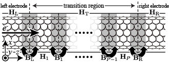
Fujimoto and Hirose developed the overbridging boundary matching (OBM) method based on the RSFD formalismFujimoto and Hirose (2003) by exploiting the advantages for electron-transport calculations, where a whole system is divided along the direction (see Fig. 1) into three regions: the left electrode, the transition region and the right electrode. The electron-transport calculation refers only to subsets of the Green’s function matrix of the transition region. In the OBM method, the subsets are calculated efficiently using a shifted conjugate-gradient (SCG) solverIwase et al. (2015) since the Hamiltonian matrix in the RSFD formalism is sparse. In the SCG solver, the computational cost for calculating the subsets is when the algorithm proposed by Takayama et al.Takayama et al. (2006) is adopted, where and are the numbers of grid points in the plane and the direction, respectively, and denotes the number of energy values to be treated at once by the SCG method. For systems with a large , the computational cost for matrix-vector operations, which is , becomes dominant.111Although the computational cost of the subsets of the Green’s function matrix is generally dominant, the cost of coefficient matrix-vector operations dominates in the case that becomes close to the eigenvalue of the truncated Hamiltonian matrix. The matrix-vector operation cost also becomes dominant when is large because the density of the eigenvalues in energy increases. Although the maximum order of the computational cost is reduced from to by the OBM method, the transport calculation has room for further reducing the computational cost to handle more realistic and longer one-dimensional systems.
In this letter, we propose an efficient computational procedure based on RSFD formalism to evaluate the electron-transport properties of long systems containing more than 100,000 atoms without accuracy deterioration. We verify the computational accuracy and performance of the proposed method. Additionally, to exemplify the efficiency of the proposed procedure we demonstrate large-scale electron-transport calculations for double-walled carbon nanotubes (DWCNTs) composed of 196,608 atoms, which make, to the best of our knowledge, the largest system in the first-principles electron-transport calculation.
Thouless and Kirkpatrick proposed an efficient calculation of subsets of a Green’s function matrix for a transition region within TB formalism as the recursive Green’s function (RGF) method.Thouless and Kirkpatrick (1981) The RGF method constructs a transition region by arranging multiple parts along the direction as illustrated in Fig. 1, and calculates only necessary subsets by recursively combining the Green’s function matrices of the adjoining small parts one by one. Since the calculation of the Green’s function matrices for the small parts is less costly than that for the extended transition region, the RGF method is capable of handling large systems and is widely used for calculating the transport properties of atomic-basis models and TB models.Lewenkopf and Mucciolo (2013); *JComputPhys215-000741; Ferry and Goodnick (1997); Sols (1995); Metalidis (2007); Souza et al. (2012); Shin et al. (2016); Rojas et al. (2019)
Now, we discuss the advantage of the RGF method in transport calculations within RSFD formalism. The transport properties are evaluated using the Green’s function of the transition region suspended between semi-infinite electrodes, , which is constructed by the Green’s function associated with the truncated transition region, , and the self-energy terms of the electrodes.Ono et al. (2012) The Green’s function matrix , in which is the truncated Hamiltonian matrix of the extended transition region consisting of parts (see Fig. 1), is expressed within the framework of RSFD formalism using the norm-conserving pseudopotentials (NCPPs) as
| (1) |
where is the truncated Hamiltonian matrix for the transition region of the th part. For simplicity, we assume that all ( have the same dimension, the interactions between the second- and further-neighboring parts are zero, and the non-zero matrix, , represents the interaction between the adjoining parts. We define the dimensions of and as and , respectively, with ; denotes an -dimensional identity matrix.
Since the Hamiltonian matrix of RSFD formalism is highly sparse, it is more advantageous to calculate the subsets of Green’s function matrix of the transition region by iterative solvers than it is to compute the entire Green’s function by direct inversions of the Hamiltonian matrix. According to Ref. Ono et al., 2012, the electron-transport properties can be estimated using submatrices located at the four corners of the Green’s function matrix, . Now we will combine the two adjoining parts to derive the Green’s function matrix associated with a truncated Hamiltonian composed of the th and ()th parts, which is denoted by the -dimensional matrix . As described in Supplemental Material, the submatrices located at the upper-left, upper-right, lower-left, and lower-right corners of are given as
| (2) | |||
| (3) | |||
| (4) | |||
| (5) |
respectively. denotes an -dimensional identity matrix, and represents the -dimensional Green’s function matrix associated with , that is, , with being an -dimensional identity matrix. As shown in Eqs. (2)–(5), we only need the four corners of , which are efficiently obtained by using the SCG method. In most cases, , with being the order of the finite-difference approximation.Chelikowsky et al. (1994a); *PRL72-001240 Repeating this procedure to connect the parts numbered from though to , we can construct the four submatrices of a -dimensional matrix .
Now, we estimate the computational cost of the proposed method. We assume that (see Fig. 1) and for are -dimensional square matrices with . In the case of the RGF method based on the atomic-basis formalism, is dense; that is, is not sufficiently smaller than . Therefore, the iterative solvers are not more efficient than direct inversion, and there is not much benefit in using Eqs. (2)–(5) to reduce the computational cost. Furthermore, the overlap matrix is generally not any scalar matrix; hence, the SCG method cannot be used to solve the linear systems. However, the RGF algorithm must be compatible with RSFD formalism since is a block-diagonal matrix and a sparse matrix.Hirose et al. (2005); Chelikowsky et al. (1994a, b) The proposed method can be implemented without negatively affecting the benefit of the SCG method, in which the matrix-vector operations for shifted energy points are omitted, and only the matrix elements of subsets are updated for shifted energy points during SCG iteration. The computational cost of the matrix-vector products with a sparse matrix increases linearly with , and the number of SCG iterations is proportional to . Therefore, the computational cost for the extended transition region is reduced from to using the RGF and the SCG methods since the cost is for each of the parts; that is, the increase in computational cost can be suppressed linearly for . Although the computational cost for calculating Eqs. (2)–(5) is , where , with being sufficiently smaller than . Consequently, further computational cost reduction for is achieved by making use of the advantages of the RGF method and SCG method within the RSFD formalism in comparison with the conventional procedure.Ono et al. (2012)
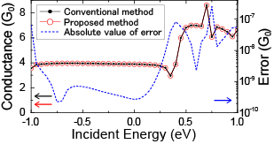
We evaluated the computational error between the conductance spectra using the Green’s function matrices obtained by the proposed method and the conventional methodOno et al. (2012) for the BN-doped (4,4)@(8,8) DWCNT to verify that the proposed method does not deteriorate the computational accuracy. The unit cell contains 192 atoms, and boron and nitrogen atoms are substitutionally co-doped into the outer tube along the circumferential direction. The dimensions are and . For this verification, a supercell has twice the dimension in the direction that of the unit cell, that is, . Using the electronic structure calculation code rspaceHirose et al. (2005); Ono and Hirose (2005) based on RSFD formalism within the DFT framework, the effective potential of the unit cell is calculated with -points, , , , the NCPPs,Kobayashi (1999); Troullier and Martins (1991); *PRL48-001425 and the local-density approximation (LDA).Vosko et al. (1980) The Green’s function calculation is collectively performed using the SCG method with . Figure 2 shows the conductance spectra of the supercell evaluated using the proposed method with and the conventional method. There are no notable errors more than .
Finally, we compared the computational times in calculating the Green’s function submatrices for several systems using the proposed method with those using the conventional method. Here the computational times are measured for systems in which (001) Si bulk is doped with B atoms. We consider a primitive unit cell of (001) Si bulk, which contains four Si atoms and has the dimensions of and . We measured the CPU time for calculating the submatrices of the Green’s function matrix in a supercell with , in which the unit cells are arranged along the direction, ( and 8), and any of the four Si atoms in each unit cell is randomly replaced with a B atom. The effective potential of the unit cell is calculated using the rspace code with -points, , , , the NCPPs, and the LDA. We prepared small parts with by duplicating the unit cell times in the direction with , and 4 to verify the influence of the cross-sectional size on the CPU time. As summarized in Table 1, the CPU time for calculating the four submatrices of with using the proposed method increases in proportion to . We confirmed that the proposed method enabled us to notably reduce the computational cost and avoid computational difficulties in handling long systems. Furthermore, one can see that the time ratio is not attenuated even in large cross-sectional systems. Since the proposed method has high weak-scaling efficiency for increasing , the benefit of this method becomes more remarkable as the system size increases.
| calculating | combining | time | ||
|---|---|---|---|---|
| time (sec.) | time (sec.) | ratio | ||
| (1,1) | 1 | 175 | – | 1.00 |
| 2 | 352 | 19 | 2.12 | |
| 4 | 669 | 56 | 4.15 | |
| 8 | 1,347 | 130 | 8.45 | |
| (2,2) | 1 | 13,381 | – | 1.00 |
| 2 | 26,773 | 1,457 | 2.11 | |
| 4 | 49,171 | 4,372 | 4.00 | |
| 8 | 98,240 | 10,206 | 8.10 | |
| (4,4) | 1 | 592,191 | – | 1.00 |
| 2 | 1,183,461 | 65,451 | 2.11 | |
| 4 | 2,159,101 | 196,408 | 3.98 | |
| 8 | 4,317,207 | 458,096 | 8.06 |
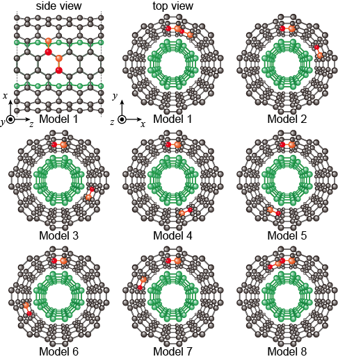
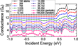
With the above verifications, it is confirmed that electron-transport properties can be estimated efficiently without the deterioration of computational accuracy using the proposed method. As a practical demonstration of the method, we investigated the electron-transport properties of DWCNTs depending on the tube length. As illustrated in Fig. 3, eight DWCNT unit-cell models with different relative positions of the two BN dimers are prepared. Here, the transport properties are evaluated for a model in which the same unit cells (Model 4) are periodically combined (periodic model) and in which different unit cells (Model 1–8) are randomly arranged (random model). For the periodic model, the transport calculations are performed for the DWCNTs with – to investigate the changes in the conductance spectrum according to the number of unit cells in the transition region. The numerical conditions and procedures to obtain the effective potential of each unit cell are the same as those mentioned above. Here, we ignore the electron-phonon couplings and evaluate the transport properties described in the ballistic regime.Ishii et al. (2010)
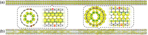
As shown in Fig. 4, for systems with small , the conductance quantization is observed at the low incident energy, where there are four conduction channels with a transmission probability of almost unity. In the low energy region, the incident electrons flow through the intra-states of the inner and outer tubes, as depicted in Fig. 5(a). Therefore, there are high-transmission channels due to the inner-tube states that are insensitive to the scattering potential created by the BN dimers in the outer tube. However, the channel transmissions are notably reduced at the high incident energy because of the inter-states between the inner and outer tubes, as illustrated in Fig. 5(b). As increases, dips appear in the conductance spectra even at the low incident energy, and they gradually become prominent. This reflects the energy gap in the energy band structure that appears in an infinite DWCNT with a periodic scattering potential, as in the Kronig-Penney model. On the contrary, for the random model with (196,608 atoms, ), overall conductance is suppressed as plotted in Fig. 4. Although the transmission in most conduction channels is notably reduced due to the random scattering potential component widely distributed in DWCNT, there are still channels with high transmission to which the intra-states of the inner tube contribute. Here, the random model with is prepared by randomly combining four different random models with and 96. We also performed calculations using random models with different configurations, but the results are essentially the same. Performing the large-scale electron-transport calculation, we can discover this difference in the conductance spectra between the randomly and periodically doped models.
In summary, we developed an efficient first-principles algorithm for evaluating the electron-transport properties of long systems consisting of a vast number of atoms. The Green’s function of the whole transition region extended towards the transport direction was obtained by recursively combining the Green’s functions of the adjoining parts one by one. The computational cost for calculating the submatrices of the Green’s functions required to estimate the transport properties is proportional to the number of the combined parts. As a practical application, we demonstrated the electron-transport calculations of BN-doped DWCNTs containing up to 196,608 atoms. The proposed method develops our understanding of experimental studies on the research and development of devices using low-dimensional materials, as reported by Refs. Franklin and Chen, 2010; Franklin et al., 2010; Qiu et al., 2017; Sun et al., 2019; Schmidt et al., 2019. Moreover, even in a submicron scale structure containing millions of atoms, it is possible to efficiently evaluate the electron-transport properties without any deterioration of computational accuracy.
Acknowledgements.
This work was partially supported by the financial support from MEXT as a social and scientific priority issue (creation of new functional devices and highperformance materials to support next-generation industries) to be tackled by using post-K computer and JSPS KAKENHI Grant Numbers JP16H03865, JP18K04873. S.T. acknowledges the financial support from Deutsche Forschungsgemeinschaft through the project numbers 389895192 and 277146847. The numerical calculations were carried out using the system B and the system C of the Institute for Solid State Physics at the University of Tokyo, the Oakforest-PACS of the Center for Computational Sciences at University of Tsukuba, and the K computer provided by the RIKEN Advanced Institute for Computational Science through the HPCI System Research project (Project ID: hp190172).References
- Kong et al. (2000) J. Kong, N. R. Franklin, C. Zhou, M. G. Chapline, K. C. S. Peng, and H. Dai, Science 287, 622 (2000).
- Duan et al. (2001) X. Duan, Y. Huang, Y. Cui, J. Wang, and C. M. Lieber, Nature 409, 66 (2001).
- Kind et al. (2002) H. Kind, H. Yan, B. Messer, M. Law, and P. Yang, Adv. Mater. 14, 158 (2002).
- Li et al. (2006) Y. Li, F. Qian, J. Xiang, and C. M. Lieber, Mater. Today 9, 18 (2006).
- Patolsky et al. (2006) F. Patolsky, G. Zheng, and C. M. L. Lieber, Anal. Chem. 78, 4260 (2006).
- Liao et al. (2006) Z.-M. Liao, Y.-D. Li, J. Xu, J.-M. Zhang, K. Xia, and D.-P. Yu, Nano Lett. 6, 1087 (2006).
- Ivanovskaya et al. (2007) V. V. Ivanovskaya, C. Köhler, and G. Seifert, Phys. Rev. B 75, 075410 (2007).
- Kohn (1999) W. Kohn, Rev. Mod. Phys. 71, 1253 (1999).
- Hohenberg and Kohn (1964) P. Hohenberg and W. Kohn, Phys. Rev. 136, B864 (1964).
- Kohn and Sham (1965) W. Kohn and L. J. Sham, Phys. Rev. 140, A1133 (1965).
- Gunst et al. (2017) T. Gunst, T. Markussen, M. L. N. Palsgaard, K. Stokbro, and M. Brandbyge, Phys. Rev. B 96, 161404(R) (2017).
- Ducry et al. (2019) F. Ducry, M. H. Bani-Hashemian, and M. Luisier, in 2019 International Conference on Simulation of Semiconductor Processes and Devices (SISPAD) (2019) pp. 1–4.
- Calogero et al. (2019) G. Calogero, N. Papior, M. Koleini, M. H. L. Larsen, and M. Brandbyge, Nanoscale 11, 6153 (2019).
- Jippo et al. (2016) H. Jippo, T. Ozaki, S. Okada, and M. Ohfuchi, J. Appl. Phys. 120, 154301 (2016).
- Fujimoto and Hirose (2003) Y. Fujimoto and K. Hirose, Phys. Rev. B 67, 195315 (2003).
- Hirose et al. (2005) K. Hirose, T. Ono, Y. Fujimoto, and S. Tsukamoto, First-Principles Calculations in Real-Space Formalism (Imperial College Press, London, 2005).
- Ono et al. (2012) T. Ono, Y. Egami, and K. Hirose, Phys. Rev. B 86, 195406 (2012).
- Iwase et al. (2015) S. Iwase, T. Hoshi, and T. Ono, Phys. Rev. E 91, 063305 (2015).
- Egami et al. (2015) Y. Egami, S. Iwase, S. Tsukamoto, T. Ono, and K. Hirose, Phys. Rev. E 92, 033301 (2015).
- Ono and Tsukamoto (2016) T. Ono and S. Tsukamoto, Phys. Rev. B 93, 045421 (2016).
- Tsukamoto et al. (2017) S. Tsukamoto, T. Ono, K. Hirose, and S. Blügel, Phys. Rev. E 95, 033309 (2017).
- Tsukamoto et al. (2018a) S. Tsukamoto, T. Ono, and S. Blügel, Phys. Rev. B 97, 115450 (2018a).
- Tsukamoto et al. (2018b) S. Tsukamoto, T. Ono, S. Iwase, and S. Blügel, Phys. Rev. B 98, 195422 (2018b).
- Egami et al. (2019) Y. Egami, S. Tsukamoto, and T. Ono, Phys. Rev. B 100, 075413 (2019).
- Takayama et al. (2006) R. Takayama, T. Hoshi, T. Sogabe, S.-L. Zhang, and T. Fujiwara, Phys. Rev. B 73, 165108 (2006).
- Note (1) Although the computational cost of the subsets of the Green’s function matrix is generally dominant, the cost of coefficient matrix-vector operations dominates in the case that becomes close to the eigenvalue of the truncated Hamiltonian matrix. The matrix-vector operation cost also becomes dominant when is large because the density of the eigenvalues in energy increases.
- Thouless and Kirkpatrick (1981) D. J. Thouless and S. Kirkpatrick, J. Phys. C: Solid State Phys. 14, 235 (1981).
- Lewenkopf and Mucciolo (2013) C. H. Lewenkopf and E. R. Mucciolo, J. Comput. Electron. 12, 203 (2013).
- Drouvelis et al. (2006) P. Drouvelis, P. Schmelcher, and P. Bastian, J. Comput. Phys. 215, 741 (2006).
- Ferry and Goodnick (1997) D. K. Ferry and S. M. Goodnick, Transport in nanostructures (Cambridge University Press, Cambridge, 1997) Chap. 3, p. 174.
- Sols (1995) F. Sols, in Quantum Transport in Ultrasmall Devices, NATO Science Series: B, Vol. 342, edited by D. K. Ferry, H. L. Grubin, C. Jacoboni, and A.-P. Jauho (Springer US, Boston, MA, 1995) pp. 329–338.
- Metalidis (2007) G. Metalidis, Electronic Transport in Mesoscopic Systems, Ph.D. thesis, Martin-Luther-Universität Halle-Wittenberg (2007).
- Souza et al. (2012) A. M. Souza, A. R. Rocha, A. Fazzio, and A. J. R. da Silva, AIP Adv. 2, 032115 (2012).
- Shin et al. (2016) M. Shin, W. J. Jeong, and J. Lee, J. Appl. Phys. 119, 154505 (2016).
- Rojas et al. (2019) W. Y. Rojas, C. E. P. Villegas, and A. R. Rocha, Phys. Chem. Chem. Phys. 21, 26027 (2019).
- Chelikowsky et al. (1994a) J. R. Chelikowsky, N. Troullier, K. Wu, and Y. Saad, Phys. Rev. B 50, 11355 (1994a).
- Chelikowsky et al. (1994b) J. R. Chelikowsky, N. Troullier, and Y. Saad, Phys. Rev. Lett. 72, 1240 (1994b).
- Ono and Hirose (2005) T. Ono and K. Hirose, Phys. Rev. B 72, 085115 (2005).
- Kobayashi (1999) K. Kobayashi, Comput. Mater. Sci. 14, 72 (1999).
- Troullier and Martins (1991) N. Troullier and J. L. Martins, Phys. Rev. B 43, 1993 (1991).
- Kleinman and Bylander (1982) L. Kleinman and D. M. Bylander, Phys. Rev. Lett. 48, 1425 (1982).
- Vosko et al. (1980) S. H. Vosko, L. Wilk, and M. Nusair, Can. J. Phys. 58, 1200 (1980).
- Ishii et al. (2010) H. Ishii, N. Kobayashi, and K. Hirose, Phys. Rev. B 82, 085435 (2010).
- Franklin and Chen (2010) A. D. Franklin and Z. Chen, Nature Nanotechnol. 5, 858 (2010).
- Franklin et al. (2010) A. D. Franklin, M. Luisier, S.-J. Han, G. Tulevski, C. M. Breslin, L. Gignac, M. S. Lundstrom, and W. Haensch, Nano Lett. 10, 758 (2010).
- Qiu et al. (2017) C. Qiu, Z. Zhang, M. Xiao, Y. Yang, D. Zhong, and L.-M. Peng, Science 355, 271 (2017).
- Sun et al. (2019) Y. Sun, Z. Peng, H. Li, Z. Wang, Y. Mu, G. Zhang, S. Chen, S. Liu, G. Wang, C. Liu, L. Sun, B. Man, and C. Yang, Biosens. Bioelectron. 137, 255 (2019).
- Schmidt et al. (2019) M. E. Schmidt, M. Muruganathan, T. Kanzaki, T. Iwasaki, A. M. M. Hammam, S. Suzuki, S. Ogawa, and H. Mizuta, Small 15, 1903025 (2019).