Efficient circular Dyson Brownian motion algorithm
Abstract
Circular Dyson Brownian motion describes the Brownian dynamics of particles on a circle (periodic boundary conditions), interacting through a logarithmic, long-range two-body potential. Within the log-gas picture of random matrix theory, it describes the level dynamics of unitary (“circular”) matrices. A common scenario is that one wants to know about an initial configuration evolved over a certain interval of time, without being interested in the intermediate dynamics. Numerical evaluation of this is computationally expensive as the time-evolution algorithm is accurate only on short time intervals because of an underlying perturbative approximation. This work proposes an efficient and easy-to-implement improved circular Dyson Brownian motion algorithm for the unitary class (Dyson index , physically corresponding to broken time-reversal symmetry). The algorithm allows one to study time evolution over arbitrarily large intervals of time at a fixed computational cost, with no approximations being involved.
I Introduction
Brownian motion describes the stochastic dynamics of microscopic particles in a thermal environment [1, 2]. It connects a broad variety of topics, including thermal physics, hydrodynamics, reaction kinetics, fluctuation phenomena, statistical thermodynamics, osmosis, and colloid science [3]. Brownian motion is intimately related to random matrix theory, which plays a key role in the understanding of quantum statistical mechanics and quantum chaos [4, 5, 6]. Random matrices have eigenvalue statistics that typically can be studied using the so-called log-gas picture [7, 8]. For matrices with real eigenvalues, the joint probability distribution of the eigenvalues is then written as a Boltzmann factor
| (1) |
where is a normalization constant that has the interpretation of a partition function, and is a parameter known as the Dyson index that has the interpretation of an inverse temperature. The Hamiltonian describes a collection of classical massless particles on a line (the eigenvalues) repelling each other over long ranges through a logarithmic two-body potential, held together by a confining background potential.
The log-gas picture describes long-range interacting particles. It has been found, for example, to accurately describe the level statistics across the many-body localization transition [9]. As the Hamiltonian in Eq. (1) does not contain a kinetic term, the particles obey non-trivial dynamics. The equilibrium as well as the non-equilibrium dynamics of the particles (“level dynamics”) are described by a phenomenon referred to as Dyson Brownian motion [10, 11]. Dyson Brownian motion turns out to provide a good description rather generically when long-range interactions are involved. As such, these dynamics (as well as the corresponding stochastic evolution of the eigenstates [12, 13]) have found applications in studies on, for example, disordered systems [14, 15, 16, 17], random matrix models [18, 19, 20, 21], many-body localization [22, 23], quantum information dynamics [24, 25, 26], and cosmological inflation [27, 28, 29, 30].
Circular Dyson Brownian motion for unitary (“circular”) matrices describes Dyson Brownian motion on a circle (periodic boundary conditions) and without background potential. A common scenario is that one wants to know about an initial configuration evolved over a certain interval of time, without being interested in the intermediate dynamics. Dyson Brownian motion can be evolved over a time interval of arbitrary length at a fixed computational cost, with no approximations being involved (see below for a more detailed explanation). Circular Dyson Brownian motion, however, requires extensively many evaluations over small intermediate intervals because of a perturbative approximation underlying the time-evolution algorithm. Circular Dyson Brownian motion is thus a process that is computationally expensive to simulate, which moreover is subject to a loss of accuracy with progressing time. Despite significant recent [31, 32] and less recent [33, 34, 35, 36] analytical progress on circular Dyson Brownian motion out of equilibrium, improved numerical capabilities are thus desired.
This work proposes an improved, easy-to-implement circular Dyson Brownian algorithm for the unitary class (Dyson index , corresponding to systems with broken time-reversal symmetry). The algorithm does not require intermediate evaluations, and thus operates at dramatically lower computational cost compared to the currently used algorithm. Moreover, it does not involve approximations, and is thus not subject to a loss of accuracy with progressing time. In short, it constructs the desired unitary matrices by orthonormalizing the columns of certain non-Hermitian matrices for which the elements perform Brownian motion. Similar to Dyson Brownian motion for Hermitian matrices, this Brownian motion process can be time evolved at a computational cost independent of the length of the time interval.
II Dyson Brownian motion for Hermitian and unitary matrices
One distinguishes between orthogonal (), unitary (), and symplectic () random matrix ensembles [7]. These names reflect the type of transformations under which the ensembles remain invariant. Physically, the type of invariance determines the behavior of a system under time reversal. For example, the orthogonal class correspond to time-reversal systems, whereas the unitary class correspond to systems with broken time-reversal symmetry. This section considers the unitary class, which is arguably the most convenient one.
Let be an Hermitian matrix with elements depending on time [10]. The initial condition can be either random or deterministic. Dyson Brownian motion for Hermitian matrices of the unitary class is a stochastic process described by
| (2) |
where the time step , in order for the eigenvalue dynamics to obey Dyson Brownian motion, is supposed to be small enough such that the eigenvalues of can be obtained accurately by second-order perturbation theory. Here, is a sample from the Gaussian unitary ensemble that is resampled at each evaluation. An matrix sampled from the Gaussian unitary ensemble can be constructed as
| (3) |
where is an matrix with complex-valued elements with and sampled independently from the normal distribution with mean zero and variance .
Let , where the time-dependent unitary matrix is chosen such that it diagonalizes . The Gaussian unitary ensemble is invariant under unitary transformations, meaning that can be replaced by a new sample from the Gaussian unitary ensemble. The increments of the eigenvalues when evolving from time to obey
| (4) |
where terms of order three and higher have been ignored. It can be shown that this time-evolution indeed describes a Brownian motion process, for example by writing down the corresponding Fokker-Planck equation. For , converges to a (scaled) sample from the Gaussian unitary ensemble irrespective of the initial condition .
Dyson Brownian motion can also be studied for unitary matrices [10, 33]. Let be an unitary matrix with time-dependent elements. Similar to the above, the initial condition can be either random or deterministic. Circular Dyson Brownian motion for the unitary class is generated by
| (5) |
where again is an sample from the Gaussian unitary ensemble that is re-sampled at each evaluation. For small enough , the matrix exponent can be approximated by the first-order expansion , which is invariant under unitary transformations (the second and higher-order terms are not). The matrix is thus obtained by applying infinitesimal orthonormality-preserving random rotations on the columns of . “Random” here means that rotations in each direction are equally likely, which agrees with the observation that is invariant under unitary transformations.
Let with the time-dependent unitary matrix chosen such that it diagonalizes . As before, can be replaced by a new sample from the Gaussian unitary ensemble. Circular Dyson Brownian motion of the eigenvalues entails that the increments of the eigenphases when evolving from time to are given by
| (6) |
where terms of order three and higher have been ignored. Equations (4) and (6) describe similar dynamics on a microscopic scale since . For , converges to a sample from the circular unitary ensemble irrespective of the initial condition .
III The algorithm
The Gaussian random matrix ensembles have the property that the sum of independent samples is a sample again, although with a prefactor . Equation (2) and its equivalents for the orthogonal and symplectic classes thus do not require the time step to be small. This implies that numerically obtaining from can be done in a single instance, at a computational cost independent of . Equation (5) for the evolution of unitary matrices does not allow for a similar argument since when and do not commute. Time-evolution for unitary matrices can thus naively only be accomplished by subsequently evolving over infinitesimal time intervals. Equation (5) moreover is subject to a loss of accuracy with progressing time as it describes the desired dynamics only up to first order.
The starting point in establishing an improved algorithm is the observation that a random unitary matrix (circular unitary ensemble) can be obtained by orthonormalizing a set of random vectors [37, 38]. Let be an matrix with elements with and sampled independently from the normal distribution with mean zero and unit variance. Such a matrix is known as a sample from the Ginibre unitary ensemble [8, 39]. The QR decomposition
| (7) |
decomposes in a unitary matrix and an upper-triangular matrix with real-valued diagonal elements. This decomposition is not unique. It can be made unique by fixing the signs of the diagonal elements of the upper-triangular matrix, for example, by requiring them to be non-negative. Let
| (8) |
Then, and is the QR decomposition with the upper-triangular matrix having non-negative diagonal entries. One can prove that the resulting unitary matrices obey the distribution of the circular unitary ensemble. Algorithmically, such unitary matrices are obtained by performing Gram-Schmidt orthonormalization (discussed below) on the columns of . A sample from the circular unitary ensemble can thus be obtained by orthonormalizing a set of random vectors.
Let be an unitary matrix with time-dependent elements. The goal is to express of Eq. (5) as
| (9) |
where is not necessarily small. Equation (5) indicates that the dynamics of are generated by orthonormality-preserving random rotations of the columns. Thus, interpolates between an identity matrix () and a sample from the circular unitary ensemble () in a way such that is invariant under unitary transformations. In other words, it generates a finite orthonormality-preserving random rotation of the columns of . Generalizing the above algorithm generating random unitary matrices, consider the QR decomposition
| (10) |
Here, is again a sample from the Ginibre unitary ensemble. This ensemble is invariant under unitary transformations. The parameter is some yet undetermined function of , which for small enough will be found to be equal to . The aim is to show that corresponds to of Eq. (9). In Eq. (10), the columns of result from Gram-Schmidt orthonormalization of the columns of the left-hand side,
| (11) |
In words, the -th column is obtained by substracting the projections on the first columns, followed by normalization. Columns with a higher index undergo more substractions than columns with lower indices. For , these substractions do not significantly alter the directions of the columns, which are then rotated randomly since is invariant under unitary transformations. As the columns of are rotated randomly, corresponds to of Eq. (9) for a proper choice of , provided that .
The limitation on the maximum value of can easily be overcome by adapting a different, appropriate, orthonormalization procedure. Löwdin symmetric orthonormalization is a procedure for which the columns are treated symmetrically, that is, the outcome is independent of the ordering [40]. For denoting some matrix, consider the singular value decomposition
| (12) |
Here, are unitary matrices and is a diagonal matrix with real-valued nonnegative entries. Löwdin symmetric orthonormalization gives the unitary matrix , which can be shown to be optimal in the sense that the distance
| (13) |
between the columns of and of acquires the minimal possible value [41]. This invites to consider the SVD-decomposition
| (14) |
with denoting a sample from the Ginibre unitary ensemble. If by Löwdin symmetric orthonormalization, then for unitary matrices . The Ginibre unitary ensemble is invariant under unitary transformations. These two facts combined guarantee the rotations generated by to be random. Thus, corresponds to of Eq. (9) for a proper choice of , without required to be small.
The relation between and can be established by requiring [Eq. (9)] and [Eq. (14)] to be identically distributed. For [Eq. (14)], let denote the first column (the choice for the first column is arbitrary), and consider the overlap
| (15) |
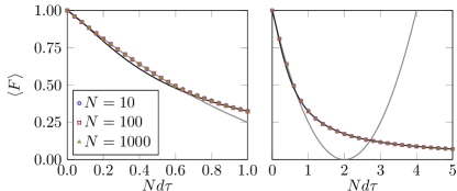
The overlap is shifted and scaled such that and . Figure 1 shows that the ensemble average of is almost perfectly described at all times already for by before and after the intersection at . These expressions have been found empirically. Next consider [Eq. (9)]. Equation (5) dictates, as can be verified numerically, that the product of two independent samples and is from the same distribution as . For defined similar as above, this means that since . Equating to the piecewise expression introduced above gives
| (16) |
which can be inverted numerically to find as a function of . Up to first order, the approximation can be made.
IV Numerical verification
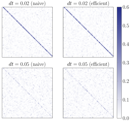
This Section provides a numerical verification of the algorithm proposed above. First, the focus is on the structure of the resulting matrices. Figure 2 shows density plots of for matrices of dimension at short () and longer () times obtained through Eq. (5) [left, “naive”] and Eqs. (9), (14), and (16) [right, “efficient”]. The initial condition is taken such that . The values of corresponding to these values of are given in the caption. One observes that the matrices on the left and right show identical characteristics.
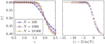
A sample from the unitary equivalent of the Rosenzweig-Porter model, considered next, can be obtained as by taking with the phases sampled independently from the uniform distribution ranging over [21]. See Refs. [42, 43] for an introduction to the Rosenzweig-Porter model and its relation to Dyson Brownian motion. Level statistics are here quantified by the average ratio of consecutive level spacings [44, 45]. For unitary matrices with ordered eigenphases , the -th ratio is defined as
| (17) |
The average is taken over all and a large number of realizations. Wigner-Dyson level statistics are characterized by , while Poissonian level statistics obey . The Rosenzweig-Porter model shows a transition (at finite dimension, a crossing) from Wigner-Dyson to Poissonian level statistics at . When plotted as a function of , the average ratio is numerically found to be independent of (finite-size collapse) [46, 21]. Figure 3 shows that the algorithm proposed in this work leads to the same results, and illustrates the capability of the algorithm proposed in this work to operate at large matrix dimensions (here, up to ). Reference [47] (Fig. 1) shows a visually indistinguishable plot obtained using Eqs. (9), (10) with the first-order approximation .
V Conclusions and outlook
Circular Dyson Brownian motion describes the Brownian dynamics of particles interacting through a long-range two-body potential in a one-dimensional environment with periodic boundary conditions. This work proposed an easy-to-implement algorithm [Eqs. (9), (14), and (16)] to simulate circular Dyson Brownian motion for the unitary class (Dyson index , physically corresponding to broken time-reversal symmetry). For short times , Eq. (14) can be replaced by the computationally cheaper Eq. (10), and the first-order approximation can be used instead of the more complicated relation (16). The latter approach is a generalization of a commonly used algorithm generating samples from the circular unitary ensemble, proposed in Refs. [37, 38]. In contrast to the currently used circular Dyson Brownian motion algorithm [Eq. (5)], here the time step does not have to be small, and no approximations have been involved. This allows one to study time-evolution over arbitrarily large time intervals at a computational cost independent of the length of the time interval, without loss of accuracy. In typical settings, this algorithm dramatically reduces the computational costs, thereby for example opening the possibility to perform detailed studies without the need for high-performance computing facilities.
An arguably interesting follow-up question would be how to modify the algorithm for the orthogonal and symplectic classes. From a sample of the circular unitary ensemble, a sample from the circular orthogonal ensemble can be obtained as [48]. It is thus tempting to hypothesize that circular Dyson Brownian motion for the orthogonal class can be simulated by the algorithm proposed in this work, and by taking the product of the transpose of the resulting unitary matrix and the resulting unitary matrix itself as the output.
Circular Dyson Brownian motion can be used to numerically generate non-ergodic unitary matrices (“unitaries”) with fractal eigenstates and a tunable degree of complexity [21, 47]. Next to what is mentioned above, this work can thus be expected to be relevant for future studies on the emergence and breakdown of statistical mechanics in the context of unitary (periodically driven) systems. It also relates to recent developments on algorithms generating random rotations [49]. Dyson Brownian motion recently attracted a spurge of interest in the context of the Brownian SYK model [50, 51, 52, 53, 54, 55, 56]. Unitary Brownian quantum systems are of current interest in the context of Brownian quantum circuits [57, 58, 59, 60, 61, 62]. This work finally can be expected to provide new opportunities in the context of the non-trivial dynamics of Brownian quantum systems.
Acknowledgements.
The author acknowledges support from the Kreitman School of Advanced Graduate Studies at Ben-Gurion University.References
- Uhlenbeck and Ornstein [1930] G. E. Uhlenbeck and L. S. Ornstein, On the theory of the Brownian motion, Phys. Rev. 36, 823 (1930).
- Wang and Uhlenbeck [1945] M. C. Wang and G. E. Uhlenbeck, On the theory of the Brownian motion II, Rev. Mod. Phys. 17, 323 (1945).
- Philipse [2018] A. P. Philipse, Brownian Motion, Undergraduate Lecture Notes in Physics (Springer Nature Switzerland, Cham, 2018).
- Mehta [1991] M. L. Mehta, Random Matrices, 2nd ed. (Academic Press, London, 1991).
- Haake [2010] F. Haake, Quantum Signatures of Chaos (Springer-Verlag, Berlin, 2010).
- D’Alessio et al. [2016] L. D’Alessio, L. Kafri, A. Polkovnikov, and M. Rigol, From quantum chaos and eigenstate thermalization to statistical mechanics and thermodynamics, Adv. Phys. 65, 239 (2016).
- Dyson [1962a] F. J. Dyson, Statistical theory of the energy levels of complex systems. I, J. Math. Phys. 3, 140 (1962a).
- Forrester [2010] P. J. Forrester, Log-Gases and Random Matrices (Princeton University Press, Princeton and Oxford, 2010).
- Buijsman et al. [2019] W. Buijsman, V. Cheianov, and V. Gritsev, Random matrix ensemble for the level statistics of many-body localization, Phys. Rev. Lett. 122, 180601 (2019).
- Dyson [1962b] F. J. Dyson, A Brownian‐motion model for the eigenvalues of a random matrix, J. Math. Phys. 3, 1191 (1962b).
- Dyson [1972] F. J. Dyson, A class of matrix ensembles, J. Math. Phys. 13, 90 (1972).
- Bourgade and Yau [2017] P. Bourgade and H.-T. Yau, The eigenvector moment flow and local quantum unique ergodicity, Comm. Math. Phys. 350, 231 (2017).
- Benigni [2021] L. Benigni, Fermionic eigenvector moment flow, Probab. Theory Relat. Fields 179, 733 (2021).
- Beenakker [1993] C. W. J. Beenakker, Brownian-motion model for parametric correlations in the spectra of disordered metals, Phys. Rev. Lett. 70, 4126 (1993).
- Narayan and Shastry [1993] O. Narayan and B. S. Shastry, Dyson’s Brownian motion and universal dynamics of quantum systems, Phys. Rev. Lett. 71, 2106 (1993).
- Shukla [1999] P. Shukla, Universal level dynamics of complex systems, Phys. Rev. E 59, 5205 (1999).
- Shukla [2005] P. Shukla, Level statistics of Anderson model of disordered systems: connection to Brownian ensembles, J. Phys. Condens. Matter 17, 1653 (2005).
- Facoetti et al. [2016] D. Facoetti, P. Vivo, and G. Biroli, From non-ergodic eigenvectors to local resolvent statistics and back: A random matrix perspective, Europhys. Lett. 115, 47003 (2016).
- von Soosten and Warzel [2018] P. von Soosten and S. Warzel, The phase transition in the ultrametric ensemble and local stability of Dyson Brownian motion, Electron. J. Probab. 23, 1 (2018).
- Kutlin and Khaymovich [2021] A. G. Kutlin and I. M. Khaymovich, Emergent fractal phase in energy stratified random models, SciPost Phys. 11, 101 (2021).
- Buijsman and Bar Lev [2022] W. Buijsman and Y. Bar Lev, Circular Rosenzweig-Porter random matrix ensemble, SciPost Phys. 12, 082 (2022).
- Serbyn and Moore [2016] M. Serbyn and J. E. Moore, Spectral statistics across the many-body localization transition, Phys. Rev. B 93, 041424(R) (2016).
- [23] C. Monthus, Level repulsion exponent for many-body localization transitions and for Anderson localization transitions via Dyson Brownian motion, J. Stat. Mech.: Theory Exp. 2016, 033113.
- Fidkowski et al. [2021] L. Fidkowski, J. Haah, and M. B. Hastings, How dynamical quantum memories forget, Quantum 5, 382 (2021).
- Schomerus [2022] H. Schomerus, Noisy monitored quantum dynamics of ergodic multi-qubit systems, J. Phys. A: Math. Theor. 55, 214001 (2022).
- [26] V. B. Bulchandani, S. L. Sondhi, and J. T. Chalker, Random-matrix models of monitored quantum circuits, J. Stat. Phys. 2024, 191.
- [27] T. Battefeld and C. Modi, Local random potentials of high differentiability to model the landscape, J. Cosmol. Astropart. Phys. 2015, 010.
- Wang and Battefeld [2016] G. Wang and T. Battefeld, Random functions via Dyson Brownian motion: progress and problems, J. Cosmol. Astropart. Phys. 2016, 008.
- Dias et al. [2016] M. Dias, J. Frazer, and M. C. D. Marsh, Simple emergent power spectra from complex inflationary physics, Phys. Rev. Lett. 117, 141303 (2016).
- [30] F. G. Pedro and A. Westphal, Inflation with a graceful exit in a random landscape, J. High Energy Phys. 2017, 163.
- Pandey et al. [2017] A. Pandey, A. Kumar, and S. Puri, Finite-range Coulomb gas models of banded random matrices and quantum kicked rotors, Phys. Rev. E 96, 052211 (2017).
- Forrester et al. [2024] P. J. Forrester, M. Kieburg, S.-H. Li, and J. Zhang, Dip-ramp-plateau for Dyson Brownian motion from the identity on , Probab. Math. Phys. 5, 321 (2024).
- Pandey and Shukla [1991] A. Pandey and P. Shukla, Eigenvalue correlations in the circular ensembles, J. Phys. A: Math. Gen. 24, 3907 (1991).
- Forrester [1996] P. J. Forrester, Some exact correlations in the Dyson Brownian motion model for transitions to the CUE, Physica A 223, 365 (1996).
- Forrester and Nagao [1998] P. J. Forrester and T. Nagao, Correlations for the circular Dyson Brownian motion model with Poisson initial conditions, Nucl. Phys. B 532, 733 (1998).
- Nagao and Forrester [2003] T. Nagao and P. J. Forrester, Dynamical correlations for circular ensembles of random matrices, Nucl. Phys. B 660, 557 (2003).
- Eaton [2007] M. L. Eaton, Multivariate Statistics: A Vector Space Approach, Lecture Notes-Monograph Series, Vol. 53 (Institute of Mathematical Statistics, Beachwood, 2007) Chap. 7.
- Mezzadri [2007] F. Mezzadri, How to generate random matrices from the classical compact groups, Not. Am. Math. Soc. 54, 592 (2007).
- Burda et al. [2014] Z. Burda, J. Grela, M. A. Nowak, W. Tarnowski, and P. Warchoł, Dysonian dynamics of the Ginibre ensemble, Phys. Rev. Lett. 113, 104102 (2014).
- Löwdin [1950] P.-O. Löwdin, On the non-orthogonality problem connected with the use of atomic wave functions in the theory of molecules and crystals, J. Chem. Phys. 18, 265 (1950).
- Pratt and Neustadter [1956] G. W. Pratt and S. F. Neustadter, Maximal orthogonal orbitals, Phys. Rev. 101, 1248 (1956).
- Rosenzweig and Porter [1960] N. Rosenzweig and C. E. Porter, “Repulsion of energy levels” in complex atomic spectra, Phys. Rev. 120, 1698 (1960).
- Kravtsov et al. [2015] V. E. Kravtsov, I. M. Khaymovich, E. Cuevas, and M. Amini, A random matrix model with localization and ergodic transitions, New J. Phys. 17, 122002 (2015).
- Oganesyan and Huse [2007] V. Oganesyan and D. A. Huse, Localization of interacting fermions at high temperature, Phys. Rev. B 75, 155111 (2007).
- Atas et al. [2013] Y. Y. Atas, E. Bogomolny, O. Giraud, and G. Roux, Distribution of the ratio of consecutive level spacings in random matrix ensembles, Phys. Rev. Lett. 110, 084101 (2013).
- Pino et al. [2019] M. Pino, J. Tabanera, and P. Serna, From ergodic to non-ergodic chaos in Rosenzweig–Porter model, J. Phys. A: Math. Theor. 52, 475101 (2019).
- Buijsman [2024] W. Buijsman, Long-range spectral statistics of the Rosenzweig-Porter model, Phys. Rev. B 109, 024205 (2024).
- Życzkowski [1993] K. Życzkowski, Parametric dynamics of quantum systems and transitions between ensembles of random matrices, Acta Phys. Pol. B 24, 967 (1993).
- Bullerjahn et al. [2023] J. T. Bullerjahn, B. Fábián, and G. Hummer, Efficient generation of random rotation matrices in four dimensions, Phys. Rev. E 108, 035307 (2023).
- [50] C. Sünderhauf, L. Piroli, X.-L. Qi, N. Schuch, and J. Ignacio Cirac, Quantum chaos in the Brownian SYK model with large finite : OTOCs and tripartite information, J. High Energy Phys. 2019, 38.
- [51] S.-K. Jian and B. Swingle, Note on entropy dynamics in the Brownian SYK model, J. High Energy Phys. 2021, 042.
- [52] L. Agarwal and S. Xu, Emergent symmetry in Brownian SYK models and charge dependent scrambling, J. High Energy Phys. 2022, 045.
- [53] P. Zhang, Information scrambling and entanglement dynamics of complex Brownian Sachdev-Ye-Kitaev models, J. High Energy Phys. 2023, 105.
- [54] V. Balasubramanian, A. Kar, O. Parrikar, and H. Rajgadia, Quantum error correction from complexity in Brownian SYK, J. High Energy Phys. 2023, 071.
- Milekhin and Xu [2023] A. Milekhin and J. Xu, Revisiting Brownian SYK and its possible relations to de Sitter, arXiv:2312.03623 (2023).
- [56] A. Tiutiakina, A. De Luca, and J. De Nardis, Frame potential of Brownian SYK model of Majorana and Dirac fermions, J. High Energy Phys. 2024, 115.
- Zhou and Chen [2019] T. Zhou and X. Chen, Operator dynamics in a Brownian quantum circuit, Phys. Rev. E 99, 052212 (2019).
- Bentsen et al. [2021] G. S. Bentsen, S. Sahu, and B. Swingle, Measurement-induced purification in large- hybrid Brownian circuits, Phys. Rev. B 104, 094304 (2021).
- Vovk and Pichler [2022] T. Vovk and H. Pichler, Entanglement-optimal trajectories of many-body quantum Markov processes, Phys. Rev. Lett. 128, 243601 (2022).
- Sahu et al. [2022] S. Sahu, S.-K. Jian, G. Bentsen, and B. Swingle, Entanglement phases in large- hybrid Brownian circuits with long-range couplings, Phys. Rev. B 106, 224305 (2022).
- [61] S.-K. Jian, G. Bentsen, and B. Swingle, Linear growth of circuit complexity from Brownian dynamics, J. High Energy Phys. 2023, 190.
- Sahu and Jian [2024] S. Sahu and S.-K. Jian, Phase transitions in sampling and error correction in local Brownian circuits, Phys. Rev. A 109, 042414 (2024).