This paper was converted on www.awesomepapers.org from LaTeX by an anonymous user.
Want to know more? Visit the Converter page.

Efficient Computation of the Magnetic Polarizability Tensor Spectral Signature using POD

B.A. Wilson and P.D. Ledger
Zienkiewicz Centre for Computational Engineering, College of Engineering,
Swansea University
b.a.wilson@swansea.ac.uk, p.d.ledger@swansea.ac.uk

Abstract

Our interest lies in the identification of hidden conducting permeable objects from measurements of the perturbed magnetic field in metal detection taken over range of low frequencies. The magnetic polarizability tensor (MPT) provides a characterisation of a conducting permeable object using a small number of coefficients, has explicit formula for their calculation and a well understood frequency behaviour, which we call its spectral signature. However, to compute such signatures, and build a library of them for object classification, requires repeated solution of a direct (full order) problem, which is typically accomplished using a finite element discretisation. To overcome this issue, we propose an efficient reduced order model (ROM) using a proper orthogonal decomposition (POD) for the rapid computation of MPT spectral signatures. Our ROM benefits from output certificates, which give bounds on the accuracy of the predicted outputs with respect to the full order model solutions. To further increase the efficiency of the computation of the MPT spectral signature, we provide scaling results, which enable an immediate calculation of the signature under changes in the object size or conductivity. We illustrate our approach by application to a range of homogenous and inhomogeneous conducting permeable objects.

Keywords Metal detection; Magnetic polarizability tensor; Reduced order model; Object classification.

MSC CLASSIFICATION 65N30; 35R30; 35B30

1 Introduction

There is considerable interest in using the magnetic polarizability tensor (MPT) characterisation of conducting permeable objects to classify and identify hidden targets in metal detection. The MPT is a complex symmetric rank 2 tensor, which has 66 independent coefficients, although the number of independent coefficients for objects with rotational or reflectional symmetries is smaller [14]. Its coefficients are a function of the exciting frequency, the object’s size, its shape as well as its conductivity and permeability. Explicit formulae for computing the tensor coefficients have been derived [4, 14, 16, 17] and validated against exact solutions and measurements [15, 16]. Also, the way in which the tensor coefficients vary with the exciting frequency is theoretically well understood [17] offering improved object classification.

The frequency (or spectral) behaviour of the MPT, henceforth called its spectral signature, has been exploited in a range of different classification algorithms including simple library classification for homogeneous [5] and inhomogeneous objects [18], a kk nearest neighbours (KNN) classification algorithm [21] and machine learning approaches [33]. The MPT classification of objects has already been applied to a range of different applications including airport security screening [22, 21], waste sorting [12] and anti-personal landmine detection [27]. The aforementioned supervised classification techniques rely on a library of MPT spectral signatures to learn how to classify the objects. The purpose of this paper is to describe an efficient computational tool for computing this library.

One approach to obtaining a library of spectral signatures is to use a metal detector or dedicated measurement device to obtain MPT coefficients of different objects [38, 37, 26], however, to do so, over a range of frequencies for a large number of objects, is time consuming and will result in unavoidable measurement errors and noise. Therefore, there is considerable interest in their automated computation. By post processing finite element method (FEM) solutions to eddy current problems using commercial packages (e.g with ANSYS as in [26]) MPT coefficients can be obtained, however, improved accuracy, and a better understanding, can be gained by using the available explicit expressions for MPT coefficients, which rely on computing finite element (FE) approximations to a transmission problem [14, 16, 17]. Nevertheless, to produce an accurate MPT spectral signature, the process must be repeated for a large number of excitation frequencies leading to potentially expensive computations for fine discretisations (with small mesh spacing and high order elements). The present paper addresses this issue by proposing a reduced order model, in the form of a (projected) proper orthogonal decomposition (POD) scheme, that relies on full order model solutions computed using the established open source FE package, NGSolve, and the recently derived alternative explicit expressions formulae for the MPT coefficients [17]. The use of NGSolve [29, 28] ensures that the solutions to underlying (eddy current type) transmission problems are accurately computed using high order 𝑯(curl)\bm{H}(\text{curl}) conforming (high order edge element) discretisations (see [19, 30, 36] and references therein) and the POD technique ensures their rapid computation over sweeps of frequency.

Reduced order models (ROMs) based on POD have been successfully applied to efficiently generate solutions for new problem parameters using a small number full order model snapshots in a range of engineering applications including mechanics [23, 25], thermal problems [35, 6], fluid flow [20, 24] as well as electromagnetic problems with application to integrated circuits [13]. However, they have not been applied to the computation of MPT spectral signatures. A review of current POD techniques is provided in [11, 9].

The main novelty of the work is the application of a POD approach for the efficient and accurate computation of the MPT spectral signature and the derivation of output certificates that ensure accuracy of the reduced order predictions. This ROM approach is motivated by the previous success of POD approaches and the theoretical study [17], which shows the spectral behaviour of the MPT is characterised by a small number of functions and, hence, has a sparse representation. The practical computation requires only computing full order model solution snapshots at a small number of frequencies and the evaluation of the MPT spectral signature follows from solving a series of extremely small linear systems. A second novelty is the presentation of simple scaling results, which enable the MPT spectral signature to easily be computed from an existing set of coefficients under the scaling of an object’s conductivity or object size.

The paper is organised as follows: In Section 2, the eddy current model, which applies in metal detection, and the asymptotic expansion of the perturbed magnetic field in the presence of a conducting permeable object, which leads to the explicit expression of the MPT, is briefly reviewed. Then, in Section 3, the FE model used for full order model problem is described. Section 4 presents the POD reduced order model scheme. This is followed, in Section 5, by the derivation of results that describe the scaling of the MPT under parameter changes. Sections 6 and 7 present numerical examples of the POD scheme for computing the frequency behaviour of the MPT and examples of the scaling of the MPT under parameter changes, respectively.

2 The eddy-current model and asymptotic expansion

We briefly discuss the eddy-current model along with stating the asymptotic expansion that forms the basis of the magnetic polarizability description of conducting objects in metal detection.

2.1 Eddy-current model

The eddy current model is a low frequency approximation of the Maxwell system that neglects the displacement currents, which is valid when the frequency is small and the conductivity of the body is high. A rigorous justification of the model involves the topology of the conducting body [3]. The eddy current model is described by the system

×𝑬α\displaystyle\nabla\times\bm{E}_{\alpha} =iωμ𝑯α,\displaystyle=\mathrm{i}\omega\mu\bm{H}_{\alpha}, (1a)
×𝑯α\displaystyle\nabla\times\bm{H}_{\alpha} =𝑱0+σ𝑬α.\displaystyle=\bm{J}_{0}+\sigma\bm{E}_{\alpha}. (1b)

where 𝑬α\bm{E}_{\alpha} and 𝑯α\bm{H}_{\alpha} are the electric and magnetic interaction fields, respectively, 𝑱0\bm{J}_{0} is an external current source, i:=1\mathrm{i}:=\sqrt{-1}, ω\omega is the angular frequency, μ\mu is the magnetic permeability and σ\sigma is the electric conductivity. We will use the eddy current model for describing the forward and inverse problems associated with metal detection.

2.1.1 Forward problem

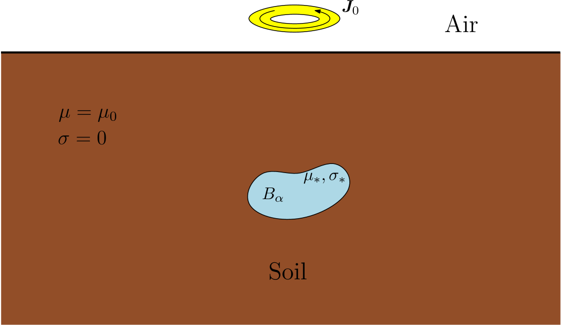
In the forward (or direct) problem, the position and materials of the conducting body BαB_{\alpha} are known. The object has a high conductivity, σ=σ\sigma=\sigma_{*}, and a permeability, μ=μ\mu=\mu_{*}. For the purpose of this study, the conducting body is assumed to be buried in soil, which is assumed to be of a much lower conductivity so that σ0\sigma\approx 0 and have a permeability μ=μ0:=4π×107H/m\mu=\mu_{0}:=4\pi\times 10^{-7}\text{H/m}. A background field is generated by a solenodial current source 𝑱0\bm{J}_{0} with support in the air above the soil, which also has σ=0\sigma=0 and μ=μ0\mu=\mu_{0}. The region around the object is Bαc:=3BαB_{\alpha}^{c}\vcentcolon=\mathbb{R}^{3}\setminus B_{\alpha} as shown in Figure 1. Note that a similar model also applies in the situation of identifying hidden targets in security screening [22, 21] and waste sorting  [12] amongst others.

Refer to caption
Figure 1: A diagram showing a hidden conducting object BαB_{\alpha}, buried in soil, with a current source located in the air above.

The forward model is described by the system (1), which holds in 3{\mathbb{R}}^{3}, with

μ(𝒙)={μ𝒙Bαμ0𝒙Bαc,σ(𝒙)={σ𝒙Bα0𝒙Bαc,\displaystyle\mu(\bm{x})=\left\{\begin{array}[]{ll}\mu_{*}&\bm{x}\in B_{\alpha}\\ \mu_{0}&\bm{x}\in B_{\alpha}^{c}\end{array}\right.,\qquad\sigma(\bm{x})=\left\{\begin{array}[]{ll}\sigma_{*}&\bm{x}\in B_{\alpha}\\ 0&\bm{x}\in B_{\alpha}^{c}\end{array}\right., (6)

and the regions BαB_{\alpha} and BαcB_{\alpha}^{c} are coupled by the transmission conditions

[𝒏×𝑬α]Γα=[𝒏×𝑯α]Γα=𝟎,\displaystyle\left[\bm{n}\times\bm{E}_{\alpha}\right]_{\Gamma_{\alpha}}=\left[\bm{n}\times\bm{H}_{\alpha}\right]_{\Gamma_{\alpha}}=\bm{0}, (7)

which hold on Γα:=Bα\Gamma_{\alpha}:=\partial B_{\alpha}. In the above, [u]Γα:=u|+u|[u]_{\Gamma_{\alpha}}:=u|_{+}-u|_{-} denotes the jump, the ++ refers to just outside of BαB_{\alpha} and the - to just inside and 𝒏\bm{n} denotes a unit outward normal to Γα\Gamma_{\alpha}.

The electric interaction field is non-physical in BαcB_{\alpha}^{c} and, to ensure uniqueness of this field, the condition 𝑬α=0\nabla\cdot\bm{E}_{\alpha}=0 is imposed in this region. Furthermore, we also require that 𝑬α=O(1/|𝒙|)\bm{E}_{\alpha}=O(1/|\bm{x}|) and 𝑯α=O(1/|𝒙|)\bm{H}_{\alpha}=O(1/|\bm{x}|) as |𝒙||\bm{x}|\to\infty, denoting that the fields go to zero at least as fast as 1/|𝒙|1/|\bm{x}|, although, in practice, this rate can be faster.

2.1.2 Inverse problem

In metal detection, the inverse problem is to determine the location, shape and material properties (σ\sigma_{*} and μ\mu_{*}) of the conducting object BαB_{\alpha} from measurements of (𝑯α𝑯0)(𝒙)(\bm{H}_{\alpha}-\bm{H}_{0})(\bm{x}) taken at a range of locations 𝒙\bm{x} in the air. As described in the introduction, there are considerable advantages in using spectral data, i.e. additionally measuring (𝑯α𝑯0)(𝒙)(\bm{H}_{\alpha}-\bm{H}_{0})(\bm{x}) over a range of frequencies ω\omega, within the limit of the eddy current model. Here, 𝑯0\bm{H}_{0} denotes the background magnetic field and 𝑬0\bm{E}_{0} and 𝑯0\bm{H}_{0} are the solutions of (1) with σ=0\sigma=0 and μ=μ0\mu=\mu_{0} in 3{\mathbb{R}}^{3}. Similar to above, we also require the decay conditions 𝑬0=O(1/|𝒙|)\bm{E}_{0}=O(1/|\bm{x}|) and 𝑯0=O(1/|𝒙|)\bm{H}_{0}=O(1/|\bm{x}|) as |𝒙||\bm{x}|\to\infty. Note that practical metal detectors measure a voltage perturbation, which corresponds to S𝒏(𝑯α𝑯0)(𝒙)d𝒙\int_{S}\bm{n}\cdot(\bm{H}_{\alpha}-\bm{H}_{0})(\bm{x})\mathrm{d}\bm{x} over an appropriate surface SS [16]. For very small coils, this voltage perturbation is approximated by 𝒎(𝑯α𝑯0)(𝒙)\bm{m}\cdot(\bm{H}_{\alpha}-\bm{H}_{0})(\bm{x}) where 𝒎\bm{m} is the magnetic dipole moment of the coil [16].

A traditional approach to the solution of this inverse problem involves creating a discrete set of voxels, each with unknown σ\sigma and μ\mu, and posing the solution to the inverse problem as an optimisation process in which σ\sigma and μ\mu are found through minimisation of an appropriate functional e.g. [32]. From the resulting images of σ\sigma and μ\mu one then attempts to infer the shape and position of the object. However, this problem is highly ill-posed [8] and presents considerable challenges mathematically and computationally in the case of limited noisy measurement data.

Instead, we seek an approximation of the perturbation (𝑯α𝑯0)(𝒙)(\bm{H}_{\alpha}-\bm{H}_{0})(\bm{x}) at some point 𝒙\bm{x} exterior to BαB_{\alpha}, which allows objects to be characterised by a small number of coefficients in a MPT that are easily obtained from the measurements of (𝑯α𝑯0)(𝒙)(\bm{H}_{\alpha}-\bm{H}_{0})(\bm{x}) once the object position is known, which can be found from a MUSIC algorithm for example [4]. The object identification then reduces to a classification problem, as discussed in the introduction.

2.2 The asymptotic expansion and MPT description
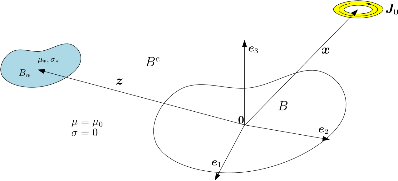
Following [4, 14] we define Bα:=αB+𝒛B_{\alpha}:=\alpha B+\bm{z} where BB is a unit size object, α\alpha is the object size and 𝒛\bm{z} is the object’s translation from the origin as shown in Figure  2.

Refer to caption
Figure 2: A diagram showing the physical description of BαB_{\alpha} with respect to the coordinate axes.

Then, using the asymptotic formula obtained by Ammari, Chen, Chen, Garnier and Volkov [4], Ledger and Lionheart  [14] have derived the simplified form

(𝑯α𝑯0)(𝒙)i=(𝑫𝒙2G(𝒙,𝒛))ij()jk(𝑯0(𝒛))k+O(α4),\displaystyle(\bm{H}_{\alpha}-\bm{H}_{0})(\bm{x})_{i}=(\bm{D}_{\bm{x}}^{2}G(\bm{x},\bm{z}))_{ij}(\mathcal{M})_{jk}(\bm{H}_{0}(\bm{z}))_{k}+O(\alpha^{4}), (8)

which holds as α0\alpha\to 0 and makes the MPT explicit. The relationship between the leading order term in the above to the dipole expansion of (𝑯α𝑯0)(𝒙)(\bm{H}_{\alpha}-\bm{H}_{0})(\bm{x}) is discussed in [16]. In the above, G(𝒙,𝒛):=1/4π|𝒙𝒛|G(\bm{x},\bm{z}):=1/{4\pi|\bm{x}-\bm{z}|} is the free space Laplace Green’s function, 𝑫x2G\bm{D}^{2}_{x}G denotes the Hessian of GG and Einstein summation convention of the indices is implied. In addition, =()jk𝒆j𝒆k{\mathcal{M}}=({\mathcal{M}})_{jk}{\bm{e}}_{j}\otimes{\bm{e}}_{k}, where 𝒆i\bm{e}_{i} denotes the iith orthonormal unit vector, is the symmetric rank 2 MPT, which describes the shape and material properties of the object BαB_{\alpha} and is frequency dependent, but is independent of the object’s position 𝒛\bm{z}. We will sometimes write [αB,ω]\mathcal{M}[\alpha B,\omega] to emphasise this. The above formulation, and the definition of {\mathcal{M}} below, are presented for the case of a single homogenous object BB, the extension to multiple inhomogeneous objects can be found in [18, 17].

Using the derivation in [17], we state the explicit formulae for the computation of the coefficients of \mathcal{M}, which are particularly well suited to a FEM discretisation. The earlier explicit expressions in [14, 15, 16] are equivalent for exact fields. We use the splitting ()ij:=(𝒩0)ij+()ij+i()ij(\mathcal{M})_{ij}:=(\mathcal{N}^{0})_{ij}+(\mathcal{R})_{ij}+\mathrm{i}(\mathcal{I})_{ij} obtained in  [17] with

(𝒩0[αB])ij\displaystyle(\mathcal{N}^{0}[\alpha B])_{ij} :=α3δijB(1μr1)d𝝃+α34BBcμ~r1×𝜽~i(0)×𝜽~j(0)d𝝃,\displaystyle:=\alpha^{3}\delta_{ij}\int_{B}(1-\mu_{r}^{-1})\mathrm{d}\bm{\xi}+\frac{\alpha^{3}}{4}\int_{B\cup B^{c}}\tilde{\mu}_{r}^{-1}\nabla\times\tilde{\bm{\theta}}_{i}^{(0)}\cdot\nabla\times\tilde{\bm{\theta}}_{j}^{(0)}\ \mathrm{d}\bm{\xi}, (9a)
([αB,ω])ij\displaystyle(\mathcal{R}[\alpha B,\omega])_{ij} :=α34BBcμ~r1×𝜽j(1)×𝜽i(1)¯d𝝃,\displaystyle:=-\frac{\alpha^{3}}{4}\int_{B\cup B^{c}}\tilde{\mu}_{r}^{-1}\nabla\times\bm{\theta}_{j}^{(1)}\cdot\nabla\times\overline{\bm{\theta}_{i}^{(1)}}\ \mathrm{d}\bm{\xi}, (9b)
([αB,ω])ij\displaystyle(\mathcal{I}[\alpha B,\omega])_{ij} :=α34Bν(𝜽j(1)+(𝜽~j(0)+𝒆j×𝝃))(𝜽i(1)+(𝜽~i(0)+𝒆i×𝝃)¯)d𝝃,\displaystyle:=\frac{\alpha^{3}}{4}\int_{B}\nu\Big{(}\bm{\theta}_{j}^{(1)}+(\tilde{\bm{\theta}}_{j}^{(0)}+\bm{e}_{j}\times\bm{\xi})\Big{)}\cdot\Big{(}\overline{\bm{\theta}_{i}^{(1)}+(\tilde{\bm{\theta}}_{i}^{(0)}+\bm{e}_{i}\times\bm{\xi})}\Big{)}\ \mathrm{d}\bm{\xi}, (9c)

where 𝒩0[αB]\mathcal{N}^{0}[\alpha B], [αB,ω]\mathcal{R}[\alpha B,\omega] and [αB,ω]\mathcal{I}[\alpha B,\omega] are real symmetric rank 2 tensors, which each have real eigenvalues. In the above,

μ~r(𝝃):={μr:=μ/μ0𝝃B1𝝃Bc,\displaystyle\tilde{\mu}_{r}(\bm{\xi}):=\left\{\begin{array}[]{ll}\mu_{r}:=\mu_{*}/\mu_{0}&\bm{\xi}\in B\\ 1&\bm{\xi}\in B^{c}\end{array}\right., (12)

and ν:=α2ωμ0σ\nu:=\alpha^{2}\omega\mu_{0}\sigma_{*}, δij\delta_{ij} is the Kronecker delta and the overbar denotes the complex conjugate. The computation of (9) rely on the solution of the transmission problems [17]

×μ~r1×𝜽i(0)\displaystyle\nabla\times\tilde{\mu}_{r}^{-1}\nabla\times\bm{\theta}_{i}^{(0)} =𝟎\displaystyle=\bm{0} in BBc,\displaystyle\textrm{in }B\cup B^{c}, (13a)
𝜽i(0)\displaystyle\nabla\cdot\bm{\theta}_{i}^{(0)} =0\displaystyle=0 in BBc,\displaystyle\textrm{in }B\cup B^{c}, (13b)
[𝒏×𝜽i(0)]Γ\displaystyle[{\bm{n}}\times\bm{\theta}_{i}^{(0)}]_{\Gamma} =𝟎\displaystyle=\bm{0} on Γ,\displaystyle\textrm{on }\Gamma, (13c)
[𝒏×μ~r1×𝜽i(0)]Γ\displaystyle[{\bm{n}}\times\tilde{\mu}_{r}^{-1}\nabla\times\bm{\theta}_{i}^{(0)}]_{\Gamma} =𝟎\displaystyle=\bm{0} on Γ,\displaystyle\textrm{on }\Gamma, (13d)
𝜽i(0)𝒆i×𝝃\displaystyle\bm{\theta}_{i}^{(0)}-{\bm{e}}_{i}\times\bm{\xi} =𝑶(|𝝃|1)\displaystyle=\bm{O}(|\bm{\xi}|^{-1}) as |𝝃|,\displaystyle\textrm{as }|\bm{\xi}|\rightarrow\infty, (13e)

where Γ:=B\Gamma:=\partial B and

×μr1×𝜽i(1)iν(𝜽i(0)+𝜽i(1))\displaystyle\nabla\times{\mu}_{r}^{-1}\nabla\times\bm{\theta}_{i}^{(1)}-\mathrm{i}\nu(\bm{\theta}_{i}^{(0)}+\bm{\theta}_{i}^{(1)}) =𝟎\displaystyle=\bm{0} in B,\displaystyle\textrm{in }B, (14a)
××𝜽i(1)\displaystyle\nabla\times\nabla\times\bm{\theta}_{i}^{(1)} =𝟎\displaystyle=\bm{0} in Bc,\displaystyle\textrm{in }B^{c}, (14b)
𝜽i(1)\displaystyle\nabla\cdot\bm{\theta}_{i}^{(1)} =0\displaystyle=0 in Bc,\displaystyle\textrm{in }B^{c}, (14c)
[𝒏×𝜽i(1)]Γ\displaystyle[{\bm{n}}\times\bm{\theta}_{i}^{(1)}]_{\Gamma} =𝟎\displaystyle=\bm{0} on Γ,\displaystyle\textrm{on }\Gamma, (14d)
[𝒏×μ~r1×𝜽i(1)]Γ\displaystyle[{\bm{n}}\times\tilde{\mu}_{r}^{-1}\nabla\times\bm{\theta}_{i}^{(1)}]_{\Gamma} =𝟎\displaystyle=\bm{0} on Γ,\displaystyle\textrm{on }\Gamma, (14e)
𝜽i(1)\displaystyle\bm{\theta}_{i}^{(1)} =𝑶(|𝝃|1)\displaystyle=\bm{O}(|\bm{\xi}|^{-1}) as |𝝃|.\displaystyle\textrm{as }|\bm{\xi}|\rightarrow\infty. (14f)

Note also that we choose to introduce 𝜽~i(0):=𝜽i(0)𝒆i×𝝃\tilde{\bm{\theta}}_{i}^{(0)}\vcentcolon=\bm{\theta}_{i}^{(0)}-{\bm{e}}_{i}\times\bm{\xi}, which can be shown to satisfy the same transmission problem as (13) except with a non-zero jump condition for [𝒏×μ~r1×𝜽~i(0)]Γ[{\bm{n}}\times\tilde{\mu}_{r}^{-1}\nabla\times\tilde{\bm{\theta}}_{i}^{(0)}]_{\Gamma} and the decay condition 𝜽~i(0)(𝝃)=𝑶(|𝝃|1)\tilde{\bm{\theta}}_{i}^{(0)}(\bm{\xi})=\bm{O}(|\bm{\xi}|^{-1}) as |𝝃||\bm{\xi}|\rightarrow\infty.

3 Full order model

To approximate the solutions to the transmission problems (13) and (14) we truncate the unbounded domain BcB^{c} at a finite distance from the object BB and create a bounded domain Ω\Omega containing BB. On Ω\partial\Omega, we approximate the decay conditions (13e) and (14f) by 𝒏×𝜽~i(0)=𝒏×(𝜽i(0)𝒆i×𝝃)=𝟎\bm{n}\times\tilde{\bm{\theta}}_{i}^{(0)}=\bm{n}\times({\bm{\theta}}_{i}^{(0)}-\bm{e}_{i}\times\bm{\xi})=\bm{0} and 𝒏×𝜽i(1)=𝟎\bm{n}\times{\bm{\theta}}_{i}^{(1)}=\bm{0}, respectively. On this finite domain, we approximate the associated weak variational statements to these problems using FEM with a 𝑯(curl)\bm{H}(\text{curl}) conforming discretisation with mesh spacing hh and order elements pp where

𝑯(curl):={𝒖:𝒖(L2(Ω))3,×𝒖(L2(Ω))3},\bm{H}(\text{curl}):=\left\{{\bm{u}}:{\bm{u}}\in(L^{2}(\Omega))^{3},\ \nabla\times{\bm{u}}\in(L^{2}(\Omega))^{3}\right\}, (15)

and L2(Ω)L^{2}(\Omega) denotes the standard space of square integrable functions. In Section 3.1 we provide their weak formulations and provide their discretisation in Section 3.2. Henceforth, we call this discrete approximation the full order model.

3.1 Weak formulation of the problem

Following the approach advocated in [19] for magnetostatic and eddy current problems, we add a regularisation term εΩ𝜽~i(0)𝝍d𝝃\varepsilon\int_{\Omega}\tilde{\bm{\theta}}_{i}^{(0)}\cdot\bm{\psi}\mathrm{d}\bm{\xi}, where ε\varepsilon is a small regularisation parameter, to the weak variational statement of (13), written in terms of 𝜽~i(0)\tilde{\bm{\theta}}_{i}^{(0)}, in order to circumvent the Coulomb gauge 𝜽~i(0)=0\nabla\cdot\tilde{\bm{\theta}}_{i}^{(0)}=0. For details of the small error induced by this approximation see [19, 36]. Then, by choosing an appropriate set of 𝑯(curl)\bm{H}(\text{curl}) conforming finite element functions in W(hp)𝑯(curl)W^{(hp)}\subset\bm{H}(\text{curl}), we obtain the following discrete regularised weak form for (13) : Find real solutions 𝜽~i(0,hp)YεW(hp)\tilde{\bm{\theta}}_{i}^{(0,hp)}\in Y^{\varepsilon}\cap W^{(hp)} such that

Ωμ~r1×𝜽~i(0,hp)×𝝍(hp)d𝝃\displaystyle\int_{\Omega}\tilde{\mu}_{r}^{-1}\nabla\times\tilde{\bm{\theta}}_{i}^{(0,hp)}\cdot\nabla\times\bm{\psi}^{(hp)}\mathrm{d}\bm{\xi} +εΩ𝜽~i(0,hp)𝝍(hp)d𝝃\displaystyle+\varepsilon\int_{\Omega}\tilde{\bm{\theta}}_{i}^{(0,hp)}\cdot\bm{\psi}^{(hp)}\mathrm{d}\bm{\xi}
=2B(1μr1)𝒆i×𝝍(hp)d𝝃,\displaystyle=2\int_{B}(1-\mu_{r}^{-1})\bm{e}_{i}\cdot\nabla\times\bm{\psi}^{(hp)}\mathrm{d}\bm{\xi}, (16)

for all 𝝍(hp)YεW(hp)\bm{\psi}^{(hp)}\in Y^{\varepsilon}\cap W^{(hp)}, where

Yε={𝒖𝑯(curl):𝒏×𝒖=𝟎 on Ω}.Y^{\varepsilon}=\Big{\{}\bm{u}\in\bm{H}(\text{curl}):{\bm{n}}\times{\bm{u}}=\bm{0}\textrm{ on }\partial\Omega\Big{\}}.

In a similar manner, the discrete weak variational statement of (14) is: Find complex solutions 𝜽i(1,hp)YεW(hp){\bm{\theta}}_{i}^{(1,hp)}\in Y^{\varepsilon}\cap W^{(hp)} such that

Ω(μr1×𝜽i(1,hp))\displaystyle\int_{\Omega}\big{(}\mu_{r}^{-1}\nabla\times\bm{\theta}_{i}^{(1,hp)}\big{)} (×𝝍(hp)¯)d𝝃iBν𝜽i(1,hp)𝝍(hp)¯d𝝃\displaystyle\cdot\big{(}\nabla\times\overline{\bm{\psi}^{(hp)}}\big{)}\mathrm{d}\bm{\xi}-\mathrm{i}\int_{B}\nu\bm{\theta}_{i}^{(1,hp)}\cdot\overline{\bm{\psi}^{(hp)}}\mathrm{d}\bm{\xi}
+εΩB𝜽i(1,hp)𝝍(hp)¯d𝝃=iBν𝜽i(0,hp)𝝍(hp)¯d𝝃,\displaystyle+\varepsilon\int_{\Omega\setminus B}\bm{\theta}_{i}^{(1,hp)}\cdot\overline{\bm{\psi}^{(hp)}}\mathrm{d}\bm{\xi}=\mathrm{i}\int_{B}\nu\bm{\theta}_{i}^{(0,hp)}\cdot\overline{\bm{\psi}^{(hp)}}\mathrm{d}\bm{\xi}, (17)

for all 𝝍(hp)YεW(hp)\bm{\psi}^{(hp)}\in Y^{\varepsilon}\cap W^{(hp)} where the overbar denotes the complex conjugate.

For what follows it is beneficial to restate (3.1) in the following form: Find 𝜽i(1,hp)YεW(hp){\bm{\theta}}_{i}^{(1,hp)}\in Y^{\varepsilon}\cap W^{(hp)} such that

a(𝜽i(1,hp),𝝍(hp);𝝎)=r(𝝍(hp);𝜽i(0,hp),𝝎),a\big{(}\bm{\theta}_{i}^{(1,hp)},\bm{\psi}^{(hp)};\bm{\omega}\big{)}=r\big{(}\bm{\psi}^{(hp)};\bm{\theta}_{i}^{(0,hp)},\bm{\omega}\big{)}, (18)

for all 𝝍(hp)YεW(hp)\bm{\psi}^{(hp)}\in Y^{\varepsilon}\cap W^{(hp)} where

a(𝜽i(1,hp),𝝍(hp);𝝎):\displaystyle a\big{(}\bm{\theta}_{i}^{(1,hp)},\bm{\psi}^{(hp)};\bm{\omega}\big{)}\vcentcolon =μ~1×𝜽i(1,hp),×𝝍(hp)L2(Ω)\displaystyle=\left<\tilde{\mu}^{-1}\nabla\times\bm{\theta}_{i}^{(1,hp)},\nabla\times{\bm{\psi}^{(hp)}}\right>_{L^{2}(\Omega)}
iν𝜽i(1,hp),𝝍(hp)L2(B)\displaystyle-\mathrm{i}\left<\nu\bm{\theta}_{i}^{(1,hp)},{\bm{\psi}^{(hp)}}\right>_{L^{2}(B)}
+ε𝜽i(1,hp),𝝍(hp)L2(ΩB),\displaystyle+\varepsilon\left<\bm{\theta}_{i}^{(1,hp)},\bm{\psi}^{(hp)}\right>_{L^{2}(\Omega\setminus B)}, (19a)
r(𝝍(hp);𝜽i(0,hp),𝝎):\displaystyle r\big{(}\bm{\psi}^{(hp)};\bm{\theta}_{i}^{(0,hp)},\bm{\omega}\big{)}\vcentcolon =iν𝜽i(0,hp),𝝍(hp)L2(B),\displaystyle=\mathrm{i}\left<\nu\bm{\theta}_{i}^{(0,hp)},{\bm{\psi}^{(hp)}}\right>_{L^{2}(B)}, (19b)

𝒖,𝒗L2(Ω):=Ω𝒖𝒗¯d𝝃\left<\bm{u},\bm{v}\right>_{L^{2}(\Omega)}:=\int_{\Omega}{\bm{u}}\cdot\overline{\bm{v}}\mathrm{d}\bm{\xi} denotes the L2L^{2} inner product over Ω\Omega and 𝝎\bm{\omega} indicates the list of the problem parameters {ω,σ,μr,α}\{\omega,\sigma_{*},\mu_{r},\alpha\} that one might wish to vary. Note that r(;,)r\big{(}\cdot;\cdot,\cdot\big{)} is a function of μr\mu_{r} as 𝜽i(0,hp)\bm{\theta}_{i}^{(0,hp)} depends on μr\mu_{r}.

3.2 Finite element discretisation

For the implementation of the full order model, we use NGSolve [1, 29, 28, 36] along with the hierarchic set of 𝑯(curl)\bm{H}(\text{curl}) conforming basis functions proposed by Schöberl and Zaglmayr [30], which are available in this software. In the following, for simplicity, we focus on the treatment of 𝜽i(1,hp)\bm{\theta}_{i}^{(1,hp)} and drop the index ii as each direction can be computed in a similar way (as can 𝜽~i(0,hp)\tilde{\bm{\theta}}_{i}^{(0,hp)}). We denote these basis functions with 𝑵(k)(𝝃)W(hp)\bm{N}^{(k)}(\bm{\xi})\in W^{(hp)} leading to the expression of the solution function along with the weighting functions

𝜽(1,hp)(𝝃,𝝎)\displaystyle\bm{\theta}^{(1,hp)}(\bm{\xi},\bm{\omega}) :=k=1Nd𝑵(k)(𝝃)qk(𝝎),\displaystyle\vcentcolon=\sum_{k=1}^{N_{d}}\bm{N}^{(k)}(\bm{\xi})\mathrm{q}_{k}(\bm{\omega}), (20a)
𝝍(hp)(𝝃,𝝎)\displaystyle\bm{\psi}^{(hp)}(\bm{\xi},\bm{\omega}) :=k=1Nd𝑵(k)(𝝃)lk(𝝎),\displaystyle\vcentcolon=\sum_{k=1}^{N_{d}}\bm{N}^{(k)}(\bm{\xi})\mathrm{l}_{k}(\bm{\omega}), (20b)

where NdN_{d} is the number of degrees of freedom. Here, and in the following, the bold italic font denotes a vector field and the bold non-italic Roman font represents a matrix (upper case) or column vector (lower case). With this distinction, we rewrite (20) in matrix form as

𝜽(1,hp)(𝝃,𝝎)\displaystyle\bm{\theta}^{(1,hp)}(\bm{\xi},\bm{\omega}) =N(𝝃)q(𝝎),\displaystyle=\textbf{N}(\bm{\xi})\textbf{q}(\bm{\omega}), (21a)
𝝍(hp)(𝝃,𝝎)\displaystyle\bm{\psi}^{(hp)}(\bm{\xi},\bm{\omega}) =N(𝝃)l(𝝎),\displaystyle=\textbf{N}(\bm{\xi})\textbf{l}(\bm{\omega}), (21b)

where N(𝝃)\textbf{N}(\bm{\xi}) is the matrix constructed with the basis vectors 𝑵k(𝝃)\bm{N}^{k}(\bm{\xi}) as its columns, i.e.

N(𝝃):=[𝑵(1)(𝝃),𝑵(2)(𝝃),,𝑵(Nd)(𝝃)].\textbf{N}(\bm{\xi})\vcentcolon=\big{[}\bm{N}^{(1)}(\bm{\xi}),\bm{N}^{(2)}(\bm{\xi}),...,\bm{N}^{(N_{d})}(\bm{\xi})\big{]}.

With this, we may also rewrite (18) as follows

i=1Ndj=1Ndli(𝝎)¯a(𝑵(j)(𝝃),𝑵(i)(𝝃);𝝎)qj(𝝎)=i=1Ndli(𝝎)¯r(𝑵(i)(𝝃);𝜽(0,hp),𝝎),\sum_{i=1}^{N_{d}}\sum_{j=1}^{N_{d}}\overline{l_{i}(\bm{\omega})}a\big{(}\bm{N}^{(j)}(\bm{\xi}),\bm{N}^{(i)}(\bm{\xi});\bm{\omega}\big{)}q_{j}(\bm{\omega})=\sum_{i=1}^{N_{d}}\overline{l_{i}(\bm{\omega})}r\big{(}\bm{N}^{(i)}(\bm{\xi});\bm{\theta}^{(0,hp)},\bm{\omega}\big{)}, (22)

and, with a suitable choice of li(𝝎)l_{i}(\bm{\omega}), we may rewrite (22) as the linear system of equations

A(𝝎)q(𝝎)=r(𝜽(0,hp),𝝎),\textbf{A}(\bm{\omega})\textbf{q}(\bm{\omega})=\textbf{r}(\bm{\theta}^{(0,hp)},\bm{\omega}), (23)

where the coefficients of 𝐀(𝝎)\bf{A}(\bm{\omega}) and 𝐫(𝜽(0,hp),𝝎){\bf r}({\bm{\theta}}^{(0,hp)},\bm{\omega}) are defined to be

(A(𝝎))ij\displaystyle(\textbf{A}(\bm{\omega}))_{ij} :=a(𝑵(j)(𝝃),𝑵(i)(𝝃);𝝎),\displaystyle\vcentcolon=a\big{(}\bm{N}^{(j)}(\bm{\xi}),\bm{N}^{(i)}(\bm{\xi});\bm{\omega}\big{)}, (24a)
(r(𝜽(0,hp),𝝎))i\displaystyle(\textbf{r}(\bm{\theta}^{(0,hp)},\bm{\omega}))_{i} :=r(𝑵(i)(𝝃);𝜽(0,hp),𝝎).\displaystyle\vcentcolon=r\big{(}\bm{N}^{(i)}(\bm{\xi});\bm{\theta}^{(0,hp)},\bm{\omega}\big{)}. (24b)

NGSolve offers efficient approaches for the computational solution to (23) using preconditioned iterative solvers [36, 19], which we exploit. Following the solution of (23), we can obtain 𝜽(1,hp)(𝝃,𝝎)\bm{\theta}^{(1,hp)}(\bm{\xi},\bm{\omega}) using (21) and, by repeating the process for i=1,2,3i=1,2,3, we get 𝜽i(1,hp)(𝝃,𝝎)\bm{\theta}_{i}^{(1,hp)}(\bm{\xi},\bm{\omega}). Then ([αB,ω,μr,σ])ij(\mathcal{M}[\alpha B,\omega,\mu_{r},\sigma_{*}])_{ij}, for the full order model, is found by using (9).

4 Reduced order model (ROM)

A traditional approach for the computation of the MPT spectral signature, i.e. the variation of the coefficients [αB,ω]{\mathcal{M}}[\alpha B,\omega] with frequency, would involve the repeated solution of the NdN_{d} sized system (23) for different ω\omega. To reduce the computational cost of this, we wish to apply a ROM in which the solution of (23) is replaced by a surrogate problem of reduced size. Thus, reducing both the computation cost and time to produce a solution for each new ω\omega. In particular, in Section 4.1, we describe a ROM based on the POD method  [9, 2, 11, 31] and, in Section 4.2, apply the variant called projection based POD (which we denote by PODP), which has already been shown to work well in the analysis of magneto-mechanical coupling applied to MRI scanners [31]. To emphasise the generality of the approach, the formulation is presented for an arbitrary list of problem parameters denoted by 𝝎\bm{\omega}. In Section 4.3 we derive a procedure for computing certificates of accuracy on the ROM solutions with negligible additional cost.

4.1 Proper orthogonal decomposition

Following the solution of (23) for 𝐪(𝝎)\mathbf{q}(\bm{\omega}) for different values of the set of parameters, 𝝎\bm{\omega}, we construct a matrix 𝐃Nd×N\mathbf{D}\in\mathbb{C}^{N_{d}\times N} with the vector of solution coefficients as its columns in the form

𝐃:=[𝐪(𝝎1),𝐪(𝝎2),,𝐪(𝝎N)],\mathbf{D}\vcentcolon=\big{[}\mathbf{q}(\bm{\omega}_{1}),\mathbf{q}(\bm{\omega}_{2}),...,\mathbf{q}(\bm{\omega}_{N})\big{]}, (25)

where NNdN\ll N_{d} denote the number of snapshots. Application of a singular value decomposition (SVD) e.g. [7, 10] gives

𝐃=𝐔𝚺𝐕,\mathbf{D}=\mathbf{U\Sigma V}^{*}, (26)

where 𝐔Nd×Nd\mathbf{U}\in\mathbb{C}^{N_{d}\times N_{d}} and 𝐕N×N\mathbf{V}^{*}\in\mathbb{C}^{N\times N} are unitary matrices and 𝚺Nd×N\mathbf{\Sigma}\in\mathbb{R}^{N_{d}\times N} is a diagonal matrix enlarged by zeros so that it becomes rectangular. In the above, 𝐕=𝐕¯T\mathbf{V}^{*}=\overline{\mathbf{V}}^{T} is the hermitian of 𝐕\mathbf{V}.

The diagonal entries (𝚺)ii=σi(\mathbf{\Sigma})_{ii}=\sigma_{i} 111Note that σ\sigma_{*} is used for conductivity and σi\sigma_{i} for a singular value, however, it should be clear from the application as to which definition applies are the singular values of 𝐃\mathbf{D} and they are arranged as σ1>σ2>>σN\sigma_{1}>\sigma_{2}>...>\sigma_{N}. Based on the sparse representation of the solutions to (14) as function of ν\nu, and hence ω\omega, (and hence also the sparse representation of the MPT) found in [17], we expect these to decay rapidly towards zero, which motivates the introduction of the truncated singular value decomposition (TSVD) e.g. [7, 10]

𝐃𝐃M=𝐔M𝚺M(𝐕M),\mathbf{D}\approx\mathbf{D}^{M}=\mathbf{U}^{M}\mathbf{\Sigma}^{M}(\mathbf{V}^{M})^{*}, (27)

where 𝐔MNd×M\mathbf{U}^{M}\in\mathbb{C}^{N_{d}\times M} are the first MM columns of 𝐔\mathbf{U}, 𝚺MM×M\mathbf{\Sigma}^{M}\in{\mathbb{R}}^{M\times M} is a diagonal matrix containing the first MM singular values and (𝐕M)M×N(\mathbf{V}^{M})^{*}\in{\mathbb{C}}^{M\times N} are the first MM rows of 𝐕\mathbf{V}^{*}. The computation of (27) constitutes the off-line stage of the POD. Using (27) we can recover an approximate representation for each of our solution snapshots as follows

𝐪(𝝎j)𝐔M𝚺M((𝐕M))j,\mathbf{q}(\bm{\omega}_{j})\approx\mathbf{U}^{M}\mathbf{\Sigma}^{M}((\mathbf{V}^{M})^{*})_{j}, (28)

where ((𝐕M))j((\mathbf{V}^{M})^{*})_{j} refers to the jjth column of (𝐕M)(\mathbf{V}^{M})^{*}.

4.2 Projection based proper orthogonal decomposition (PODP)

In the online stage of PODP, 𝐪PODP(𝝎)𝐪(𝝎)\mathbf{q}^{PODP}({\bm{\omega}})\approx\mathbf{q}({\bm{\omega}}) is obtained by taking a linear combination of the columns of 𝐔M{\bf U}^{M} where the coefficients of this projection are contained in the vector 𝐩M{\bf p}^{M}. We choose to also approximate 𝐥(𝝎)\mathbf{l}({\bm{\omega}}) in a similar way so that

𝜽(1,hp)(𝝃,𝝎)(𝜽(1,hp))PODP(𝝃,𝝎):=\displaystyle\bm{\theta}^{(1,hp)}(\bm{\xi},\bm{\omega})\approx(\bm{\theta}^{(1,hp)})^{\text{PODP}}({\bm{\xi}},\bm{\omega)}:= N(𝝃)𝐪PODP(𝝎)=N(𝝃)𝐔MpM(𝝎)Y(PODP),\displaystyle\textbf{N}(\bm{\xi})\mathbf{q}^{PODP}({\bm{\omega}})=\textbf{N}(\bm{\xi})\mathbf{U}^{M}\textbf{p}^{M}(\bm{\omega})\in Y^{(PODP)}, (29a)
𝝍(hp)(𝝃,𝝎)(𝝍(1,hp))PODP(𝝃,𝝎):=\displaystyle\bm{\psi}^{(hp)}(\bm{\xi},\bm{\omega})\approx(\bm{\psi}^{(1,hp)})^{\text{PODP}}({\bm{\xi}},\bm{\omega)}:= N(𝝃)lPODP(𝝎)=N(𝝃)𝐔MoM(𝝎)Y(PODP),\displaystyle\textbf{N}(\bm{\xi})\textbf{l}^{PODP}(\bm{\omega})=\textbf{N}(\bm{\xi})\mathbf{U}^{M}\textbf{o}^{M}(\bm{\omega})\in Y^{(PODP)}, (29b)

where Y(PODP)YεW(hp)\in Y^{(PODP)}\subset Y^{\varepsilon}\cap W^{(hp)}. Substituting these lower dimensional representations in to (22) we obtain the following

i=1Mj=1MoiM(𝝎)¯a(𝑵(j)(𝝃)(𝐔M)j\displaystyle\sum_{i=1}^{M}\sum_{j=1}^{M}\overline{o^{M}_{i}(\bm{\omega})}a\big{(}\bm{N}^{(j)}(\bm{\xi})(\mathbf{U}^{M})_{j} ,𝑵(i)(𝝃)(𝐔M)i;𝝎)pMj(𝝎)\displaystyle,\bm{N}^{(i)}(\bm{\xi})(\mathbf{U}^{M})_{i};\bm{\omega}\big{)}p^{M}_{j}(\bm{\omega})
=i=1MoiM(𝝎)¯r(𝑵(i)(𝝃)(𝐔M)i;𝜽(0,hp),𝝎),\displaystyle=\sum_{i=1}^{M}\overline{o^{M}_{i}(\bm{\omega})}r\big{(}\bm{N}^{(i)}(\bm{\xi})(\mathbf{U}^{M})_{i};\bm{\theta}^{(0,hp)},\bm{\omega}\big{)},
(𝐨M(𝝎))((𝐔M)𝐀(𝝎)𝐔M)𝐩M(𝝎)\displaystyle({\mathbf{o}^{M}}(\bm{\omega}))^{*}((\mathbf{U}^{M})^{*}\mathbf{A}(\bm{\omega})\mathbf{U}^{M})\mathbf{p}^{M}(\bm{\omega}) =(𝐨M(𝝎))(𝐔M)𝐫(𝜽(0,hp),𝝎).\displaystyle=({\mathbf{o}^{M}}(\bm{\omega}))^{*}(\mathbf{U}^{M})^{*}\mathbf{r}(\bm{\theta}^{(0,hp)},\bm{\omega}). (30)

Then, if we choose 𝐨M(𝝎)\mathbf{o}^{M}(\bm{\omega}) appropriately, we obtain the linear system

𝐀M(𝝎)𝐩M(𝝎)=𝐫M(𝜽(0,hp),𝝎),\mathbf{A}^{M}(\bm{\omega})\mathbf{p}^{M}(\bm{\omega})=\mathbf{r}^{M}(\bm{\theta}^{(0,hp)},\bm{\omega}), (31)

which is of size M×MM\times M where 𝐀M(𝝎):=(𝐔M)𝐀(𝝎)𝐔M\mathbf{A}^{M}(\bm{\omega})\vcentcolon=(\mathbf{U}^{M})^{*}\mathbf{A}(\bm{\omega})\mathbf{U}^{M} and 𝐫M(𝜽(0,hp),𝝎):=(𝐔M)𝐫(𝜽(0,hp),𝝎)\mathbf{r}^{M}(\bm{\theta}^{(0,hp)},\bm{\omega})\vcentcolon=(\mathbf{U}^{M})^{*}\mathbf{r}(\bm{\theta}^{(0,hp)},\bm{\omega}). Note, since M<NNdM<N\ll N_{d}, this is significantly smaller than (23) and, therefore, substantially computationally cheaper to solve. After solving this reduced system, and obtaining 𝐩M(𝝎)\mathbf{p}^{M}(\bm{\omega}), we obtain an approximate solution for 𝜽(1,hp)(𝝃,𝝎)\bm{\theta}^{(1,hp)}(\bm{\xi},\bm{\omega}) using (29).

Focusing on the particular case where 𝝎=ω\bm{\omega}=\omega, from (19) we observe that we can express 𝐀\mathbf{A} and 𝐫\mathbf{r} as the simple sums

𝐀(ω)=\displaystyle\mathbf{A}(\omega)= 𝐀(0)+ω𝐀(1),\displaystyle\mathbf{A}^{(0)}+\omega\mathbf{A}^{(1)},
𝐫(𝜽(0,hp),ω)=\displaystyle\mathbf{r}(\bm{\theta}^{(0,hp)},\omega)= ω𝐫(1)(𝜽(0,hp)),\displaystyle\omega\mathbf{r}^{(1)}(\bm{\theta}^{(0,hp)}),

where the definitions of 𝐀(0)\mathbf{A}^{(0)}, 𝐀(1)\mathbf{A}^{(1)} and 𝐫(1)(𝜽(0,hp))\mathbf{r}^{(1)}(\bm{\theta}^{(0,hp)}) are obvious from (24),(19) and the definition of ν\nu. Then, by computing and storing (𝐔M)𝐀(0)𝐔M(\mathbf{U}^{M})^{*}\mathbf{A}^{(0)}\mathbf{U}^{M}, (𝐔M)𝐀(1)𝐔M(\mathbf{U}^{M})^{*}\mathbf{A}^{(1)}\mathbf{U}^{M} , (𝐔M)𝐫(1)(𝜽(0,hp))(\mathbf{U}^{M})^{*}\mathbf{r}^{(1)}(\bm{\theta}^{(0,hp)}), which are independent of ω\omega, it follows that 𝐀M(ω)\mathbf{A}^{M}({\omega}) and 𝐫M(𝜽(0,hp),ω)\mathbf{r}^{M}(\bm{\theta}^{(0,hp)},{\omega}) can be efficiently calculated for each new ω\omega from the stored data. In a similar manner, by precomputing appropriate data, the MPT coefficients in (9) can also be rapidly evaluated for each new ω\omega using the PODP solutions. This leads to further considerable computational savings. We emphasise that the PODP is only applied to obtain ROM solutions for 𝜽(1)(𝝃,ω)\bm{\theta}^{(1)}(\bm{\xi},{\omega}) and not to 𝜽(0)(𝝃)\bm{\theta}^{(0)}(\bm{\xi}), which does not depend on ω\omega.

4.3 PODP output certification

We follow the approach described in [11], which enables us to derive and compute certificates of accuracy on the MPT coefficients obtained with PODP, with respect to those obtained with full order model, as a function of ω\omega. To do this, we set ϵi(ω)=𝜽i(1,hp)(ω)(𝜽i(1,hp))PODP(ω)Y(hp)\bm{\epsilon}_{i}(\omega)=\bm{\theta}_{i}^{(1,hp)}(\omega)-(\bm{\theta}_{i}^{(1,hp)})^{\text{PODP}}(\omega)\in Y^{(hp)}, where we have reintroduced the subscript ii, as we need to distinguish between the cases i=1,2,3i=1,2,3. Although ϵi\bm{\epsilon}_{i} also depends on 𝝃\bm{\xi}, we have chosen here, and in the following, to only emphasise its dependence on ω\omega. We have also introduced Y(hp)=YεW(hp)Y^{(hp)}=Y^{\varepsilon}\cap W^{(hp)} for simplicity of notation, and note that this error satisfies

a(ϵi(ω),𝝍;ω)=r(𝝍;𝜽i(0,hp),ω)𝝍Y(hp),\displaystyle a(\bm{\epsilon}_{i}(\omega),\bm{\psi};{\omega})=r(\bm{\psi};\bm{\theta}_{i}^{(0,hp)},\omega)\qquad\forall\bm{\psi}\in Y^{(hp)}, (32)

which is called the error equation [11] and

a(ϵi(ω),𝝍;ω)=0𝝍Y(PODP),\displaystyle a(\bm{\epsilon}_{i}(\omega),\bm{\psi};\omega)=0\qquad\forall\bm{\psi}\in Y^{(PODP)}, (33)

which is called Galerkin orthogonality [11]. The Riesz representation [11] of r(;𝜽i(0,hp),ω)r(\cdot;\bm{\theta}_{i}^{(0,hp)},\omega) denoted by 𝒓^i(ω)Y(hp)\hat{\bm{r}}_{i}(\omega)\in Y^{(hp)} is such that

(𝒓^i(ω),𝝍)Y(hp)=r(𝝍;𝜽i(0,hp),ω)𝝍Y(hp),\displaystyle(\hat{\bm{r}}_{i}(\omega),\bm{\psi})_{Y^{(hp)}}=r(\bm{\psi};\bm{\theta}_{i}^{(0,hp)},\omega)\qquad\forall\bm{\psi}\in Y^{(hp)}, (34)

so that

a(ϵi(ω),𝝍;ω)=(𝒓^i(ω),𝝍)Y(hp)𝝍Y(hp).\displaystyle a(\bm{\epsilon}_{i}(\omega),\bm{\psi};{\omega})=(\hat{\bm{r}}_{i}(\omega),\bm{\psi})_{Y^{(hp)}}\qquad\forall\bm{\psi}\in Y^{(hp)}. (35)

Then, by using the alternative set of formulae for the tensor coefficients [17]

([αB,ω])ij\displaystyle(\mathcal{R}[\alpha B,\omega])_{ij} =α34BνIm(𝜽j(1,hp))𝜽i(0,hp)d𝝃=α34νIm(𝜽j(1,hp)),𝜽i(0,hp)L2(B),\displaystyle=-\frac{\alpha^{3}}{4}\int_{B}\nu\text{Im}(\bm{\theta}_{j}^{(1,hp)})\cdot\bm{\theta}_{i}^{(0,hp)}\mathrm{d}\bm{\xi}=-\frac{\alpha^{3}}{4}\left<\nu\text{Im}(\bm{\theta}_{j}^{(1,hp)}),\bm{\theta}_{i}^{(0,hp)}\right>_{L^{2}(B)}, (36a)
([αB,ω])ij\displaystyle(\mathcal{I}[\alpha B,\omega])_{ij} =α34(BνRe(𝜽j(1,hp))𝜽i(0,hp)d𝝃+Bν𝜽j(0,hp)𝜽i(0,hp)d𝝃)\displaystyle=\frac{\alpha^{3}}{4}\left(\int_{B}\nu\text{Re}(\bm{\theta}_{j}^{(1,hp)})\cdot\bm{\theta}_{i}^{(0,hp)}\mathrm{d}\bm{\xi}+\int_{B}\nu\bm{\theta}_{j}^{(0,hp)}\cdot\bm{\theta}_{i}^{(0,hp)}\mathrm{d}\bm{\xi}\right)
=α34(νRe(𝜽j(1,hp)),𝜽i(0,hp)L2(B)+ν𝜽j(0,hp),𝜽i(0,hp)L2(B)),\displaystyle=\frac{\alpha^{3}}{4}\left(\left<\nu\text{Re}(\bm{\theta}_{j}^{(1,hp)}),\bm{\theta}_{i}^{(0,hp)}\right>_{L^{2}(B)}+\left<\nu\bm{\theta}_{j}^{(0,hp)},\bm{\theta}_{i}^{(0,hp)}\right>_{L^{2}(B)}\right), (36b)

written in terms of the full order solutions, we obtain the certificates for the tensor entries computed using PODP stated in the lemma below. Note that the formulae stated in (9) are used for the actual POD computation of (PODP[αB,ω])ij(\mathcal{R}^{PODP}[\alpha B,\omega])_{ij} and (PODP[αB,ω])ij(\mathcal{I}^{PODP}[\alpha B,\omega])_{ij}, but the form in (36) is useful for obtaining certificates. Also, as (𝒩[αB])ij(\mathcal{N}[\alpha B])_{ij} is independent of ω\omega we have (𝒩0,PODP[αB])ij=(𝒩0[αB])ij(\mathcal{N}^{0,PODP}[\alpha B])_{ij}=(\mathcal{N}^{0}[\alpha B])_{ij} and we write PODP[αB,ω]=𝒩0,PODP[αB]+PODP[αB,ω]+iPODP[αB,ω]\mathcal{M}^{PODP}[\alpha B,\omega]=\mathcal{N}^{0,PODP}[\alpha B]+\mathcal{R}^{PODP}[\alpha B,\omega]+\mathrm{i}\mathcal{I}^{PODP}[\alpha B,\omega] for the MPT obtained by PODP.

Lemma 4.1.

An error certificate for the tensor coefficients computed using PODP is

|([αB,ω])ij(PODP[αB,ω])ij|\displaystyle\left|(\mathcal{R}[\alpha B,\omega])_{ij}-(\mathcal{R}^{PODP}[\alpha B,\omega])_{ij}\right|\leq (Δ[ω])ij,\displaystyle(\Delta[\omega])_{ij}, (37a)
|([αB,ω])ij(PODP[αB,ω])ij|\displaystyle\left|(\mathcal{I}[\alpha B,\omega])_{ij}-(\mathcal{I}^{PODP}[\alpha B,\omega])_{ij}\right|\leq (Δ[ω])ij,\displaystyle(\Delta[\omega])_{ij}, (37b)

where

(Δ[ω])ij:=α38αLB(𝒓^i(ω)Y(hp)2+𝒓^j(ω)Y(hp)2+𝒓^i(ω)𝒓^j(ω)Y(hp)2),\displaystyle(\Delta[\omega])_{ij}:=\frac{\alpha^{3}}{8\alpha_{LB}}\left(\|\hat{\bm{r}}_{i}(\omega)\|_{Y^{(hp)}}^{2}+\|\hat{\bm{r}}_{j}(\omega)\|_{Y^{(hp)}}^{2}+\|\hat{\bm{r}}_{i}(\omega)-\hat{\bm{r}}_{j}(\omega)\|_{Y^{(hp)}}^{2}\right),

and αLB\alpha_{LB} is a lower bound on a stability constant.

Proof.

We concentrate on the proof for |([αB,ω])ij(PODP[αB,ω])ij|\left|(\mathcal{R}[\alpha B,\omega])_{ij}-(\mathcal{R}^{PODP}[\alpha B,\omega])_{ij}\right| as the proof for the second bound is similar and leads to the same result. Recalling the symmetry of [αB,ω]\mathcal{R}[\alpha B,\omega], we have ([αB,ω])ij=12(([αB,ω])ij+([αB,ω])ji)(\mathcal{R}[\alpha B,\omega])_{ij}=\frac{1}{2}\left((\mathcal{R}[\alpha B,\omega])_{ij}+(\mathcal{R}[\alpha B,\omega])_{ji}\right) so that

D:=|([αB,ω])ij(PODP[αB,ω])ij|=\displaystyle D:=\left|(\mathcal{R}[\alpha B,\omega])_{ij}-(\mathcal{R}^{PODP}[\alpha B,\omega])_{ij}\right|= α38|νIm(ϵi),𝜽j(0,hp)L2(B)+νIm(ϵj),𝜽i(0,hp)L2(B)|\displaystyle\frac{\alpha^{3}}{8}\left|\left<\nu\text{Im}(\bm{\epsilon}_{i}),\bm{\theta}_{j}^{(0,hp)}\right>_{L^{2}(B)}+\left<\nu\text{Im}(\bm{\epsilon}_{j}),\bm{\theta}_{i}^{(0,hp)}\right>_{L^{2}(B)}\right|
=\displaystyle= α38|νIm(ϵi),𝜽i(0,hp)L2(B)+νIm(ϵi),𝜽j(0,hp)𝜽i(0,hp)L2(B)+\displaystyle\frac{\alpha^{3}}{8}\left|\left<\nu\text{Im}(\bm{\epsilon}_{i}),\bm{\theta}_{i}^{(0,hp)}\right>_{L^{2}(B)}+\left<\nu\text{Im}(\bm{\epsilon}_{i}),\bm{\theta}_{j}^{(0,hp)}-\bm{\theta}_{i}^{(0,hp)}\right>_{L^{2}(B)}+\right.
νIm(ϵj),𝜽j(0,hp)L2(B)+νIm(ϵj),𝜽i(0,hp)𝜽j(0,hp)L2(B)|\displaystyle\left.\left<\nu\text{Im}(\bm{\epsilon}_{j}),\bm{\theta}_{j}^{(0,hp)}\right>_{L^{2}(B)}+\left<\nu\text{Im}(\bm{\epsilon}_{j}),\bm{\theta}_{i}^{(0,hp)}-\bm{\theta}_{j}^{(0,hp)}\right>_{L^{2}(B)}\right|
=\displaystyle= α38|νIm(ϵi),𝜽i(0,hp)L2(B)+νIm(ϵiϵj),𝜽j(0,hp)𝜽i(0,hp)L2(B)+\displaystyle\frac{\alpha^{3}}{8}\left|\left<\nu\text{Im}(\bm{\epsilon}_{i}),\bm{\theta}_{i}^{(0,hp)}\right>_{L^{2}(B)}+\left<\nu\text{Im}(\bm{\epsilon}_{i}-\bm{\epsilon}_{j}),\bm{\theta}_{j}^{(0,hp)}-\bm{\theta}_{i}^{(0,hp)}\right>_{L^{2}(B)}+\right.
νIm(ϵj),𝜽j(0,hp)L2(B)|,\displaystyle\left.\left<\nu\text{Im}(\bm{\epsilon}_{j}),\bm{\theta}_{j}^{(0,hp)}\right>_{L^{2}(B)}\right|,

which follows since ν\nu and 𝜽i(0,hp)\bm{\theta}_{i}^{(0,hp)} are real valued and where we have dropped the dependence of ω\omega on ϵi\bm{\epsilon}_{i} for simplicity of presentation. Thus,

Dα38(|νϵi,𝜽i(0,hp)L2(B)|+|ν(ϵiϵj),𝜽j(0,hp)𝜽i(0,hp)L2(B)|+|νϵj,𝜽j(0,hp)L2(B)|).\displaystyle D\leq\frac{\alpha^{3}}{8}\left(\left|\left<\nu\bm{\epsilon}_{i},\bm{\theta}_{i}^{(0,hp)}\right>_{L^{2}(B)}\right|+\left|\left<\nu(\bm{\epsilon}_{i}-\bm{\epsilon}_{j}),\bm{\theta}_{j}^{(0,hp)}-\bm{\theta}_{i}^{(0,hp)}\right>_{L^{2}(B)}\right|+\left|\left<\nu\bm{\epsilon}_{j},\bm{\theta}_{j}^{(0,hp)}\right>_{L^{2}(B)}\right|\right).

Next, using (32), we make the observation that

|νϵi,𝜽i(0,hp)L2(B)|=|r(ϵi;𝜽i(0,hp),ω)|=|a(ϵi,ϵi;ω)|=ϵiω2.\displaystyle\left|\left<\nu\bm{\epsilon}_{i},\bm{\theta}_{i}^{(0,hp)}\right>_{L^{2}(B)}\right|=\left|r(\bm{\epsilon}_{i};\bm{\theta}_{i}^{(0,hp)},\omega)\right|=\left|a(\bm{\epsilon}_{i},\bm{\epsilon}_{i};{\omega})\right|=\|\bm{\epsilon}_{i}\|_{\omega}^{2}.

Also, since r(𝝍;𝜽j(0,hp)𝜽i(0,hp),ω)=a(𝜽j(1,hp)(ω)𝜽i(1,hp)(ω),𝝍;ω)=a(ϵjϵi,𝝍;ω)r(\bm{\psi};\bm{\theta}_{j}^{(0,hp)}-\bm{\theta}_{i}^{(0,hp)},\omega)=a(\bm{\theta}_{j}^{(1,hp)}(\omega)-\bm{\theta}_{i}^{(1,hp)}(\omega),\bm{\psi};\omega)=a(\bm{\epsilon}_{j}-\bm{\epsilon}_{i},\bm{\psi};\omega) for all 𝝍Y(hp)\bm{\psi}\in Y^{(hp)}, we have |ν𝝍,𝜽j(0,hp)𝜽i(0,hp)L2(B)|=|a(ϵjϵi,𝝍;ω)|\left|\left<\nu\bm{\psi},\bm{\theta}_{j}^{(0,hp)}-\bm{\theta}_{i}^{(0,hp)}\right>_{L^{2}(B)}\right|=\left|a(\bm{\epsilon}_{j}-\bm{\epsilon}_{i},\bm{\psi};\omega)\right| so that

|ν(ϵiϵj),𝜽j(0,hp)𝜽i(0,hp)L2(B)|=|r(ϵiϵj;𝜽j(0,hp)𝜽i(0,hp),ω)|=|a(ϵjϵi,ϵiϵj;ω)|=ϵiϵjω2,\displaystyle\left|\left<\nu(\bm{\epsilon}_{i}-\bm{\epsilon}_{j}),\bm{\theta}_{j}^{(0,hp)}-\bm{\theta}_{i}^{(0,hp)}\right>_{L^{2}(B)}\right|=\left|r(\bm{\epsilon}_{i}-\bm{\epsilon}_{j};\bm{\theta}_{j}^{(0,hp)}-\bm{\theta}_{i}^{(0,hp)},\omega)\right|=\left|a(\bm{\epsilon}_{j}-\bm{\epsilon}_{i},\bm{\epsilon}_{i}-\bm{\epsilon}_{j};{\omega})\right|=\|\bm{\epsilon}_{i}-\bm{\epsilon}_{j}\|_{\omega}^{2},

and hence

Dα38(ϵiω2+ϵiϵjω2+ϵjω2).\displaystyle D\leq\frac{\alpha^{3}}{8}\left(\|\bm{\epsilon}_{i}\|_{\omega}^{2}+\|\bm{\epsilon}_{i}-\bm{\epsilon}_{j}\|_{\omega}^{2}+\|\bm{\epsilon}_{j}\|_{\omega}^{2}\right). (38)

Following similar steps to [11, pg47-50], and introducing a Riesz representation in (34), we can find that

ϵiω2𝒓^i(ω)Y(hp)2αLB,ϵjω2𝒓^j(ω)Y(hp)2αLB,ϵiϵjω2𝒓^i(ω)𝒓^j(ω)Y(hp)2αLB,\displaystyle\|\bm{\epsilon}_{i}\|_{\omega}^{2}\leq\frac{\|\hat{\bm{r}}_{i}(\omega)\|_{Y^{(hp)}}^{2}}{\alpha_{LB}},\qquad\|\bm{\epsilon}_{j}\|_{\omega}^{2}\leq\frac{\|\hat{\bm{r}}_{j}(\omega)\|_{Y^{(hp)}}^{2}}{\alpha_{LB}},\qquad\|\bm{\epsilon}_{i}-\bm{\epsilon}_{j}\|_{\omega}^{2}\leq\frac{\|\hat{\bm{r}}_{i}(\omega)-\hat{\bm{r}}_{j}(\omega)\|_{Y^{(hp)}}^{2}}{\alpha_{LB}},

and, combining this with (38), completes the proof. ∎

The efficient evaluation of (37) follows the approach presented in [11, pg52-54], adapted to complex matrices and with the simplification that we compute a Riesz representation 𝒓^i(ω)Y(h0)\hat{\bm{r}}_{i}(\omega)\in Y^{(h0)} using lowest order elements for computational efficiency. The computations are split in to those performed in the off-line stage and those in the on-line stage as follows.

In the off-line stage, the following (2M+1)×(2M+1)(2M+1)\times(2M+1) hermitian matrices are computed

𝐆(i,j)=(W(i))HM01W(j),\displaystyle\mathbf{G}^{(i,j)}=\left(\textbf{W}^{(i)}\right)^{H}\textbf{M}_{0}^{-1}\textbf{W}^{(j)},

where, since 𝐆(j,i)=(𝐆(i,j))H\mathbf{G}^{(j,i)}=(\mathbf{G}^{(i,j)})^{H}, it follows that, in practice, only the 3 matrices 𝐆(1,1)\mathbf{G}^{(1,1)}, 𝐆(2,2)\mathbf{G}^{(2,2)} and 𝐆(3,3)\mathbf{G}^{(3,3)} are required for computing the certificates on the diagonal entries of the tensors, and the further 3 matrices 𝐆(1,2)\mathbf{G}^{(1,2)}, 𝐆(1,3)\mathbf{G}^{(1,3)} and 𝐆(2,3)\mathbf{G}^{(2,3)} are needed for the off-diagonal terms. In the above, (M0)ij=𝑵(i),𝑵(j)L2(Ω)(\textbf{M}_{0})_{ij}=\left<\bm{N}^{(i)},\bm{N}^{(j)}\right>_{L^{2}(\Omega)} are the coefficient of a real symmetric FEM mass matrix for the lowest order, with 𝑵(i),𝑵(j)W(h0)\bm{N}^{(i)},\bm{N}^{(j)}\in W^{(h0)} being typical lowest order basis functions, and

W(i):=P0p(𝐫(1)(𝜽i(0))𝐀(0)𝐔(M,i)𝐀(1)𝐔(M,i)),\displaystyle\textbf{W}^{(i)}:=\textbf{P}_{0}^{p}\left(\begin{array}[]{ccc}\mathbf{r}^{(1)}(\bm{\theta}_{i}^{(0)})&\mathbf{A}^{(0)}\mathbf{U}^{(M,i)}&\mathbf{A}^{(1)}\mathbf{U}^{(M,i)}\end{array}\right), (40)

where P0p\textbf{P}_{0}^{p} is a projection matrix of the FEM basis functions from order pp to the lowest order 0, 𝐔(M,i)\mathbf{U}^{(M,i)} is the 𝐔M\mathbf{U}^{M} obtained in (27) for the iith direction. The stability constant αLB=λminmin(1,ωω)\alpha_{LB}=\lambda_{min}\text{min}(1,\frac{\omega}{\omega^{\prime}}) is obtained from the smallest eigenvalue of an eigenvalue problem [11, pg56], which, in practice, is only performed once for smallest frequency of interest ω\omega^{\prime}.

In the on-line stage, we evaluate

𝒓^i(ω)Y(hp)2=\displaystyle\|\hat{\bm{r}}_{i}(\omega)\|_{Y^{(hp)}}^{2}= ((𝐰(i)(ω))H𝐆(i,i)(𝐰(i)(ω)))1/2,\displaystyle\left((\mathbf{w}^{(i)}(\omega))^{H}\mathbf{G}^{(i,i)}(\mathbf{w}^{(i)}(\omega))\right)^{1/2},
𝒓^i(ω)𝒓^j(ω)Y(hp)2=\displaystyle\|\hat{\bm{r}}_{i}(\omega)-\hat{\bm{r}}_{j}(\omega)\|_{Y^{(hp)}}^{2}= (𝒓^i(ω)Y(hp)2+𝒓^j(ω)Y(hp)22Re((𝐰i(ω))H𝐆(i,j)(𝐰(j)(ω))))1/2,\displaystyle\left(\|\hat{\bm{r}}_{i}(\omega)\|_{Y^{(hp)}}^{2}+\|\hat{\bm{r}}_{j}(\omega)\|_{Y^{(hp)}}^{2}-2\text{Re}((\mathbf{w}^{i}(\omega))^{H}\mathbf{G}^{(i,j)}(\mathbf{w}^{(j)}(\omega)))\right)^{1/2},

for each ω\omega by updating the vector

𝐰(i)(ω)=(ω𝐩M(ω)ω𝐩M(ω)).\mathbf{w}^{(i)}(\omega)=\left(\begin{array}[]{c}\omega\\ -\mathbf{p}^{M}({\omega})\\ -\omega\mathbf{p}^{M}({\omega})\end{array}\right).

We then apply (37) to obtain the output certificates.

5 Scaling of the MPT under parameter changes

Two results that aid the computation of the frequency sweep of an MPT for an object with scaled conductivity and an object with a scaled object size from an already known frequency sweep of the MPT for the same shaped object are stated below.

Lemma 5.1.

Given the MPT coefficients for an object αB\alpha B with material parameters μr\mu_{r} and σ\sigma_{*} at frequency sωs\omega, the coefficients of the MPT for an object, which has the same BB, α\alpha and μr\mu_{r}, but with conductivity sσs\sigma_{*}, at frequency ω\omega, are given by

([αB,ω,μr,sσ])ij=\displaystyle({\mathcal{M}}[\alpha B,\omega,\mu_{r},s\sigma_{*}])_{ij}= ([αB,sω,μr,σ])ij,\displaystyle({\mathcal{M}}[\alpha B,s\omega,\mu_{r},\sigma_{*}])_{ij}, (41)

where ([αB,sω,μr,σ])ij({\mathcal{M}}[\alpha B,s\omega,\mu_{r},\sigma_{*}])_{ij} denote the coefficients of the original MPT at frequency sωs\omega.

Proof.

This result immediately follows from (9) and (14) since both are written in terms of ν=α2σμ0ω\nu=\alpha^{2}\sigma_{*}\mu_{0}\omega. ∎

Lemma 5.2.

Given the MPT coefficients for an object αB\alpha B with material parameters μr\mu_{r} and σ\sigma_{*} at frequency s2ωs^{2}\omega, the coefficients of the MPT for an object sαBs\alpha B, which is the same as BB apart from having size sαs\alpha, at frequency ω\omega, are given by

([sαB,ω,μr,σ])ij=\displaystyle({\mathcal{M}}[s\alpha B,\omega,\mu_{r},\sigma_{*}])_{ij}= s3([αB,s2ω,μr,σ])ij,\displaystyle s^{3}({\mathcal{M}}[\alpha B,s^{2}\omega,\mu_{r},\sigma_{*}])_{ij}, (42)

where ([αB,s2ω,μr,σ])ij({\mathcal{M}}[\alpha B,s^{2}\omega,\mu_{r},\sigma_{*}])_{ij} denote the coefficients of the original MPT at frequency s2ωs^{2}\omega.

Proof.

For the case of μr=1\mu_{r}=1 this result was proved by Ammari et al. [5]. We generalise this to 0<μr<μrmax<0<\mu_{r}<\mu_{r}^{max}<\infty as follows: We use the splitting ()ij:=(𝒩0)ij(𝒞σ)ij+(𝒩σ)ij(\mathcal{M})_{ij}:=(\mathcal{N}^{0})_{ij}-(\mathcal{C}^{\sigma_{*}})_{ij}+(\mathcal{N}^{\sigma_{*}})_{ij} presented in [15] and let 𝜽i,B(0)\bm{\theta}_{i,B}^{(0)} denote the solution to (13). Then, we find that

1s𝜽i,sB(0)(s𝝃)=𝜽i,B(0)(𝝃),\frac{1}{s}\bm{\theta}_{i,sB}^{(0)}(s\bm{\xi}^{\prime})=\bm{\theta}_{i,B}^{(0)}(\bm{\xi}^{\prime}),

where 𝜽i,sB(0)\bm{\theta}_{i,sB}^{(0)} is the solution to (13) with BB replaced by sBsB. If 𝜽i,B(1)[s2ν]\bm{\theta}_{i,B}^{(1)}[s^{2}\nu] is the solution to (14) with ν\nu replaced by s2νs^{2}\nu, then, we find that

1s𝜽i,sB(1)[ν](s𝝃)=𝜽i,B(1)[s2ν](𝝃),\frac{1}{s}\bm{\theta}_{i,sB}^{(1)}[\nu](s\bm{\xi}^{\prime})=\bm{\theta}_{i,B}^{(1)}[s^{2}\nu](\bm{\xi}^{\prime}),

where 𝜽i,sB(1)[ν]\bm{\theta}_{i,sB}^{(1)}[\nu] is the solution to (14) with BB replaced by sBsB. Using the above, the definitions in Lemma 1 of [15], and 𝝃=s𝝃\bm{\xi}=s{\bm{\xi}}^{\prime} we find

(𝒞σ[α(sB),ω,μr,σ])ij=\displaystyle({\mathcal{C}}^{\sigma_{*}}[\alpha(sB),\omega,\mu_{r},\sigma_{*}])_{ij}= iα3ν4sB𝒆i(𝝃×(𝜽i,sB(1)[ν]+𝜽i,sB(0)))d𝝃\displaystyle-\frac{\mathrm{i}\alpha^{3}\nu}{4}\int_{sB}\bm{e}_{i}\cdot\left(\bm{\xi}\times\left(\bm{\theta}_{i,sB}^{(1)}[\nu]+\bm{\theta}_{i,sB}^{(0)}\right)\right)\mathrm{d}\bm{\xi}
=\displaystyle= is3α3ν4B𝒆i(s𝝃×(𝜽i,sB(1)[ν](s𝝃)+𝜽i,sB(0)(s𝝃)))d𝝃\displaystyle\frac{\mathrm{i}s^{3}\alpha^{3}\nu}{4}\int_{B}\bm{e}_{i}\cdot\left(s\bm{\xi}^{\prime}\times\left(\bm{\theta}_{i,sB}^{(1)}[\nu](s\bm{\xi}^{\prime})+\bm{\theta}_{i,sB}^{(0)}(s\bm{\xi}^{\prime})\right)\right)\mathrm{d}\bm{\xi}^{\prime}
=\displaystyle= is3α3(s2ν)4B𝒆i(𝝃×(𝜽i,B(1)[s2ν]+𝜽i,B(0)))d𝝃=s3(𝒞σ[αB,s2ω,μr,σ])ij,\displaystyle\frac{\mathrm{i}s^{3}\alpha^{3}(s^{2}\nu)}{4}\int_{B}\bm{e}_{i}\cdot\left(\bm{\xi}^{\prime}\times\left(\bm{\theta}_{i,B}^{(1)}[s^{2}\nu]+\bm{\theta}_{i,B}^{(0)}\right)\right)\mathrm{d}\bm{\xi}^{\prime}=s^{3}({\mathcal{C}}^{\sigma_{*}}[\alpha B,s^{2}\omega,\mu_{r},\sigma_{*}])_{ij},
(𝒩0[α(sB),μr])ij=\displaystyle({\mathcal{N}}^{0}[\alpha(sB),\mu_{r}])_{ij}= α32[μ~1]ΓsB𝒆iξ×𝜽i,sB(0)d𝝃\displaystyle\frac{\alpha^{3}}{2}[\tilde{\mu}^{-1}]_{\Gamma}\int_{sB}\bm{e}_{i}\cdot\nabla_{\xi}\times\bm{\theta}_{i,sB}^{(0)}\mathrm{d}\bm{\xi}
=\displaystyle= s3α32[μ~1]ΓB𝒆i1sξ×(s𝜽i,B(0))d𝝃=s3(𝒩0[αB,μr])ij,\displaystyle\frac{s^{3}\alpha^{3}}{2}[\tilde{\mu}^{-1}]_{\Gamma}\int_{B}\bm{e}_{i}\cdot\frac{1}{s}\nabla_{\xi^{\prime}}\times(s\bm{\theta}_{i,B}^{(0)})\mathrm{d}\bm{\xi}^{\prime}=s^{3}({\mathcal{N}}^{0}[\alpha B,\mu_{r}])_{ij},
(𝒩σ[α(sB),ω,μr,σ])ij=\displaystyle({\mathcal{N}}^{\sigma_{*}}[\alpha(sB),\omega,\mu_{r},\sigma_{*}])_{ij}= α32[μ~1]ΓsB𝒆iξ×𝜽i,sB(1)[ν]d𝝃\displaystyle\frac{\alpha^{3}}{2}[\tilde{\mu}^{-1}]_{\Gamma}\int_{sB}\bm{e}_{i}\cdot\nabla_{\xi}\times\bm{\theta}_{i,sB}^{(1)}[\nu]\mathrm{d}\bm{\xi}
=\displaystyle= s3α32[μ~1]ΓB𝒆i1sξ×(s𝜽i,B(1)[s2ν])d𝝃=s3(𝒩σ[αB,s2ω,μr,σ])ij,\displaystyle\frac{s^{3}\alpha^{3}}{2}[\tilde{\mu}^{-1}]_{\Gamma}\int_{B}\bm{e}_{i}\cdot\frac{1}{s}\nabla_{\xi^{\prime}}\times(s\bm{\theta}_{i,B}^{(1)}[s^{2}\nu])\mathrm{d}\bm{\xi}^{\prime}=s^{3}({\mathcal{N}}^{\sigma_{*}}[\alpha B,s^{2}\omega,\mu_{r},\sigma_{*}])_{ij},

and the quoted result immediately follows. ∎

6 Numerical examples of PODP

The PODP algorithm has been implemented in the Python interface to the high order finite element solver NGSolve package led by the group of Schöberl [29, 36, 28] available at https://ngsolve.org. The snapshots are computed by solving (3.1) and (18) using NGSolve and their 𝑯(curl)\bm{H}(\text{curl}) conforming tetrahedral finite element basis functions of order pp on meshes of spacing hh [30]. Following the solution of (23), and the application of (20), the coefficients of [αB,ω]{\mathcal{M}}[\alpha B,\omega] 222 In the following, when presenting numerical results for the PODP, we frequently choose to drop the superscript PODP on [αB,ω]\mathcal{M}[\alpha B,\omega] [αB,ω]\mathcal{R}[\alpha B,\omega], [αB,ω]\mathcal{I}[\alpha B,\omega] and 𝒩0[B]\mathcal{N}^{0}[B], introduced in Section 4.3, for brevity of presentation where no confusion arises. Also, we will return to using the notation [αB,ω,μr,σ]{\mathcal{M}}[\alpha B,\omega,\mu_{r},\sigma_{*}], which illustrates the full parameter dependence, in Section 7 when considering scaling of conductivity and object size. follow by simple post-processing of (9). If desired, PODP output certificates can also be efficiently computed using the approach described in Section 4.3. The Python scripts for the computations presented can be accessed at
https://github.com/BAWilson94/MPT-Calculator.

6.1 Conducting permeable sphere

We begin with the case where Bα=αBB_{\alpha}=\alpha B is a permeable conducting sphere of radius α=0.01\alpha=0.01 m and BB is the unit sphere centred at the origin. The sphere is chosen to have a relative permeability μr=1.5\mu_{r}=1.5 and conductivity σ=5.96×10⁶\sigma_{*}=5.96\times 10^{6} S/m. To produce the snapshots of the full order model, we set Ω\Omega to be a ball 100 times the radius of BB and discretize it using a mesh of 26 385 unstructured tetrahedral elements, refined towards the object, and a polynomial order of p=3p=3. We have chosen this discretization since it has already been found to produce an accurate representation of [αB,ω]\mathcal{M}[\alpha B,\omega] for 102<ω<10810^{2}<\omega<10^{8} rad/s by comparing with exact solution of the MPT for a sphere [34, 16]. Indeed, provided that the geometry discretisation error is under control, performing pp-refinement of the full order model solution results in exponential convergence to the true solution [14].

We follow two different schemes for choosing frequencies ω\omega for generating the solution vectors 𝐪(ω)\mathbf{q}(\omega) required for 𝐃\mathbf{D} in (25). Firstly, we consider linearly spaced frequencies ωminωnωmax\omega_{min}\leq\omega_{n}\leq\omega_{max}, n=1,2,,Nn=1,2,\ldots,N, where, as in Section 4.1, NN is the number of snapshots, and denote this choice of samples by “Lin” in the results. Secondly, we consider logarithmically spaced frequencies ωminωnωmax\omega_{min}\leq\omega_{n}\leq\omega_{max} and denote this regime by “Log” in the results.

Considering both linearly and logarithmically spaced frequencies with ωmin=1×10² rad/s\omega_{min}=1\times 10^{2}\text{ rad/s}, ωmax=1×10⁸ rad/s\omega_{max}=1\times 10^{8}\text{ rad/s} and N=9,13,17N=9,13,17, in turn, to generate the snapshots, the application of an SVD to 𝐃\mathbf{D} in (26) leads to the results shown in Figure 3 where the values have been scaled by σ1\sigma_{1} and are strictly decreasing. We observe that “Log” case produces singular values σi/σ1\sigma_{i}/\sigma_{1}, which tend to 0 with increasing ii, while the “Lin” case produces σi/σ1\sigma_{i}/\sigma_{1}, which tend to a finite constant with increasing ii. Also shown is the tolerance TOL=1×10³TOL=1\times 10^{-3}, i.e. we define MM such that σM/σ1TOL<σM+1/σ1\sigma_{M}/\sigma_{1}\leq TOL<\sigma_{M+1}/\sigma_{1} and create the matrices 𝐔M\mathbf{U}^{M}, 𝚺M\mathbf{\Sigma}^{M} and (𝐕)M(\mathbf{V}^{*})^{M} by taking the first MM columns of 𝐔\mathbf{U}, MM rows of 𝐕\mathbf{V}^{*} and first MM rows and columns of 𝚺\mathbf{\Sigma}.

Refer to captionRefer to caption(b) Linearly spaced snapshots(a) Logarithmically spaced snapshots\begin{array}[]{cc}\includegraphics[width=231.26378pt,keepaspectratio]{LinearSingularValues.pdf}&\includegraphics[width=231.26378pt,keepaspectratio]{SingularValues.pdf}\\ \textrm{\footnotesize{(b) Linearly spaced snapshots}}&\textrm{\footnotesize{(a) Logarithmically spaced snapshots}}\end{array}
Figure 3: Sphere with μr=1.5\mu_{r}=1.5, σ=5.96×10⁶\sigma_{*}=5.96\times 10^{6} S/m, α=0.01\alpha=0.01 m: PODP applied to the computation of [αB,ω]\mathcal{M}[\alpha B,\omega] showing σi/σ1\sigma_{i}/\sigma_{1} for (a)(a) linearly spaced snapshots and (b)(b) logarithmically spaced snapshots.

The superior performance of logarithmically spaced frequency snapshots over those linearly spaced is illustrated in Figure 4 (a)(a) where the variation of the condition number κ(𝐀M(ω))\kappa(\mathbf{A}^{M}(\omega)) with ω\omega for the frequency range and snapshots presented in Figure 3 is shown. Included in Figure 4 (b)(b) is the corresponding error measure |e(Λi(ω))|:=|Λiexact(ω)ΛiPODP(ω)|/|Λiexact(ω)||e(\Lambda_{i}(\omega))|:=|\Lambda_{i}^{exact}(\omega)-\Lambda_{i}^{PODP}(\omega)|/|\Lambda_{i}^{exact}(\omega)| with ω\omega, where Λi(ω)=λi([αB,ω]+𝒩0[αB])+iλi([αB,ω])\Lambda_{i}(\omega)=\lambda_{i}(\mathcal{R}[\alpha B,\omega]+{\mathcal{N}}^{0}[\alpha B])+\textrm{i}\lambda_{i}(\mathcal{I}[\alpha B,\omega]), λi()\lambda_{i}(\cdot) indicates the iith eigenvalue. Note that, since the results for i=1,2,3i=1,2,3 are identical on this scale, only i=1i=1 is shown. From the results shown in this figure, we see that, with the exception of N=17N=17, the logarithmically spaced frequency snapshots results in a lower condition number compared to the linear ones and that all the logarithmically spaced snapshots result in a smaller error.

Refer to captionRefer to caption(a) κ(𝐀M(ω))(b) e(Λi(ω))\begin{array}[]{cc}\includegraphics[width=231.26378pt,keepaspectratio]{PointsVsConditionNumber.pdf}&\includegraphics[width=231.26378pt,keepaspectratio]{PointsVsError.pdf}\\ \textrm{\footnotesize{(a) $\kappa(\mathbf{A}^{M}(\omega))$}}&\textrm{\footnotesize{(b) $e(\Lambda_{i}(\omega))$}}\end{array}
Figure 4: Sphere with μr=1.5\mu_{r}=1.5, σ=5.96×10⁶\sigma_{*}=5.96\times 10^{6} S/m, α=0.01\alpha=0.01 m: PODP applied to the computation of [αB,ω]\mathcal{M}[\alpha B,\omega] showing (a)(a) Variation of κ(𝐀M(ω))\kappa(\mathbf{A}^{M}(\omega)) with ω\omega for linearly and logarithmically spaced snapshots (b)(b) Variation of e(Λi(ω))e(\Lambda_{i}(\omega)) with ω\omega for the same snapshots.

Further tests reveal that the accuracy of the PODP using N=9,13,17N=9,13,17 and logarithmically spaced snapshots remains similar to that shown in Figure 4 (b)(b) for TOL1×103TOL\leq 1\times 10^{-3} for this problem. We complete the discussion of the sphere by showing a comparison of λi([αB,ω])\lambda_{i}(\mathcal{R}[\alpha B,\omega]) and λi([αB,ω])\lambda_{i}(\mathcal{I}[\alpha B,\omega]), each with ω\omega, for the full order model, PODP using N=9N=9 and the exact solution in Figure 5. Again, the results for i=1,2,3i=1,2,3 are identical and, hence, only i=1i=1 is shown. In this figure, we observe excellent agreement between PODP, the full order model solution and exact solution.

Refer to captionRefer to caption(a) λi(𝒩0[αB]+[αB,ω])(b) λi([αB,ω])\begin{array}[]{cc}\includegraphics[width=231.26378pt,keepaspectratio]{SphereReal.pdf}&\includegraphics[width=231.26378pt,keepaspectratio]{SphereImag.pdf}\\ \textrm{\footnotesize{(a) $\lambda_{i}(\mathcal{N}^{0}[\alpha B]+\mathcal{R}[\alpha B,\omega])$}}&\textrm{\footnotesize{(b) $\lambda_{i}(\mathcal{I}[\alpha B,\omega]$)}}\end{array}

Figure 5: Sphere with μr=1.5\mu_{r}=1.5, σ=5.96×10⁶\sigma_{*}=5.96\times 10^{6} S/m, α=0.01\alpha=0.01 m: PODP applied to the computation of [αB,ω]\mathcal{M}[\alpha B,\omega] with N=9N=9 and TOL=1×10⁴TOL=1\times 10^{-4} showing (a)(a) λi(𝒩0[αB]+[αB,ω])\lambda_{i}(\mathcal{N}^{0}[\alpha B]+\mathcal{R}[\alpha B,\omega]) and (b)(b) λi([αB,ω])\lambda_{i}(\mathcal{I}[\alpha B,\omega]) each with ω\omega.

In Figure 6, we show the output certificates (PODP[αB,ω]+𝒩0,PODP[αB])ii±(Δ[ω])ii(\mathcal{R}^{PODP}[\alpha B,\omega]+{\mathcal{N}}^{0,PODP}[\alpha B])_{ii}\pm(\Delta[\omega])_{ii} (summation of repeated indices is not implied) and (PODP[αB,ω])ii±(Δ[ω])ii(\mathcal{I}^{PODP}[\alpha B,\omega])_{ii}\pm(\Delta[\omega])_{ii}, each with ω\omega, obtained by applying the technique described in Section 4.3 for the case where i=1i=1 and with N=17,21N=17,21 and TOL=1×10⁶TOL=1\times 10^{-6}. Similar certificates can be obtained for the other tensor coefficients. We observe that certificates are indistinguishable from the the MPT coefficients obtained with PODP for low frequencies in both cases and the certificates rapidly tend to the MPT coefficients for all ω\omega as NN is increased. Note that TOL=1×10⁶TOL=1\times 10^{-6} is chosen as larger tolerances lead to larger certificates, however, this reduction in tolerance does not substantially affect the computational cost of the ROM. Although the effectivity indices (Δ[ω])11/|([αB,ω]PODP[αB,ω])11|(\Delta[\omega])_{11}/|(\mathcal{R}[\alpha B,\omega]-\mathcal{R}^{PODP}[\alpha B,\omega])_{11}| and (Δ[ω])11/|([αB,ω]PODP[αB,ω])11|(\Delta[\omega])_{11}/|(\mathcal{I}[\alpha B,\omega]-\mathcal{I}^{PODP}[\alpha B,\omega])_{11}|) of the PODP with respect to the full order model are clearly larger at higher frequencies, we emphasise that they are computed at negligible additional cost, they converge rapidly to the MPT coefficients obtained with PODP as NN is increased and give credibility in the PODP solution without the need of performing additional full order model solutions to validate the ROM.

Refer to captionRefer to caption(a) (𝒩0[αB]+[αB,ω])11N=17(b) ([αB,ω])11N=17 Refer to captionRefer to caption(c) (𝒩0[αB]+[αB,ω])11N=21(d) ([αB,ω])11N=21 \begin{array}[]{cc}\includegraphics[width=231.26378pt,keepaspectratio]{SphereErrorBarsRealn_17.pdf}&\includegraphics[width=231.26378pt,keepaspectratio]{SphereErrorBarsImagn_17.pdf}\\ \textrm{\footnotesize{(a) $(\mathcal{N}^{0}[\alpha B]+\mathcal{R}[\alpha B,\omega])_{11}$, $N=17$}}&\textrm{\footnotesize{(b) $(\mathcal{I}[\alpha B,\omega])_{11}$, $N=17$} }\\ \includegraphics[width=231.26378pt,keepaspectratio]{SphereErrorBarsRealn_21.pdf}&\includegraphics[width=231.26378pt,keepaspectratio]{SphereErrorBarsImagn_21.pdf}\\ \textrm{\footnotesize{(c) $(\mathcal{N}^{0}[\alpha B]+\mathcal{R}[\alpha B,\omega])_{11}$, $N=21$}}&\textrm{\footnotesize{(d) $(\mathcal{I}[\alpha B,\omega])_{11}$, $N=21$} }\end{array}
Figure 6: Sphere with μr=1.5\mu_{r}=1.5, σ=5.96×10⁶\sigma_{*}=5.96\times 10^{6} S/m, α=0.01\alpha=0.01 m: PODP applied to the computation of [αB,ω]\mathcal{M}[\alpha B,\omega] with TOL=1×10⁶TOL=1\times 10^{-6} showing the PODP solution, full order model solutions and output certificates ()±(Δ[ω])11(\cdot)\pm(\Delta[\omega])_{11} for (a)(a) (𝒩0[αB]+[αB,ω])11(\mathcal{N}^{0}[\alpha B]+\mathcal{R}[\alpha B,\omega])_{11} using N=17N=17, (b)(b) ([αB,ω])11(\mathcal{I}[\alpha B,\omega])_{11} using N=17N=17, (c)(c) (𝒩0[αB]+[αB,ω])11(\mathcal{N}^{0}[\alpha B]+\mathcal{R}[\alpha B,\omega])_{11} using N=21N=21 and (d)(d) ([αB,ω])11(\mathcal{I}[\alpha B,\omega])_{11} using N=21N=21, each with ω\omega.

The computational speed-ups offered by using the PODP compared to a frequency sweep performed with the full order model are shown in Figure 7 where N=9,13,17N=9,13,17 and logarithmically spaced snapshots are chosen with ωmin=1×10² rad/s\omega_{min}=1\times 10^{2}\text{ rad/s}, ωmax=1×10⁸ rad/s\omega_{max}=1\times 10^{8}\text{ rad/s}, as before. For the comparison, we vary the number of output points N0N_{0} produced in a frequency sweep and measure the time taken to produce each of these frequency sweeps using a 2.9 GHz quad core Intel i5 processor and also show the percentage speed up offered by each of these PODP sweeps. Also shown is the break down of the computational time for the offline and online stages of the PODP for the case where N=13N=13. Note, in particular, that the computational cost increases very slowly with N0N_{0} and that the additional cost involved in computing the output certificates is negligible. The breakdown of computational costs for other NN is similar.

Refer to captionRefer to caption(a) Sweep Time(b) Break Down of PODP Timings\begin{array}[]{cc}\includegraphics[width=231.26378pt,keepaspectratio]{UpdatedTimings.pdf}&\includegraphics[width=231.26378pt,keepaspectratio]{TimeBreakDown.pdf}\\ \textrm{\footnotesize{(a) Sweep Time}}&\textrm{\footnotesize{(b) Break Down of PODP Timings}}\end{array}

Figure 7: Sphere with μr=1.5\mu_{r}=1.5, σ=5.96×10⁶\sigma_{*}=5.96\times 10^{6} S/m, α=0.01\alpha=0.01 m: PODP applied to the computation of [αB,ω]\mathcal{M}[\alpha B,\omega] with N=13,17,21N=13,17,21 and TOL=1×10⁶TOL=1\times 10^{-6} showing, for different numbers of outputs N0N_{0}, (a)(a) sweep computational time compared with full order and (b)(b) a typical break down of the offline and online computational times for N=13N=13.

6.2 Conducing permeable torus

Next, we consider Bα=αBB_{\alpha}=\alpha B to be a torus where BB has major and minor radii a=2a=2 and b=1b=1, respectively, α=0.01\alpha=0.01 m and the object is permeable and conducting with μr=1.5\mu_{r}=1.5, σ=5×10⁵\sigma_{*}=5\times 10^{5} S/m. The object is centred at the origin so that it has rotational symmetry around the 𝒆1\bm{e}_{1} axis and hence [αB,ω]{\mathcal{M}}[\alpha B,\omega] has independent coefficients ([αB,ω])11({\mathcal{M}}[\alpha B,\omega])_{11} and ([αB,ω])22=([αB,ω])33({\mathcal{M}}[\alpha B,\omega])_{22}=({\mathcal{M}}[\alpha B,\omega])_{33}, and thus 𝒩0[αB]\mathcal{N}^{0}[\alpha B], [αB,ω]\mathcal{R}[\alpha B,\omega], [αB,ω]\mathcal{I}[\alpha B,\omega] each have 22 independent eigenvalues. To compute the full order model, we set Ω\Omega to be a sphere of radius 100, centred at the origin, such that it contains BB and discretise it by a mesh of 26142 unstructured tetrahedral elements, refined towards the object, and a polynomial order of p=3p=3. This discretisation has already been found to produce an accurate representation of [αB,ω]\mathcal{M}[\alpha B,\omega] for the frequency range with ωmin=1×10² rad/s\omega_{min}=1\times 10^{2}{\textrm{ rad}}{/\textrm{s}} and ωmax=1×10⁸ rad/s\omega_{max}=1\times 10^{8}{\textrm{ rad}}/{\textrm{s}} with the full order model.

The reduced order model is constructed using N=13N=13 snapshots at logarithmically spaced frequencies with TOL=1×10⁴TOL=1\times 10^{-4}. Figure 8 shows the results for λi(𝒩0[αB]+[αB,ω])\lambda_{i}(\mathcal{N}^{0}[\alpha B]+\mathcal{R}[\alpha B,\omega]) and λi([αB,ω])\lambda_{i}(\mathcal{I}[\alpha B,\omega]), each with ω\omega, for both the full order model and the PODP. The agreement is excellent in both cases.

Refer to captionRefer to caption(a) λi(𝒩0[αB]+[αB,ω])(b) λi([αB,ω])\begin{array}[]{cc}\includegraphics[width=231.26378pt,keepaspectratio]{TorusRealEigenvalues.pdf}&\includegraphics[width=231.26378pt,keepaspectratio]{TorusImaginaryEigenvalues.pdf}\\ \textrm{\footnotesize{(a) $\lambda_{i}(\mathcal{N}^{0}[\alpha B]+\mathcal{R}[\alpha B,\omega])$}}&\textrm{\footnotesize{(b) $\lambda_{i}(\mathcal{I}[\alpha B,\omega]$)}}\end{array}

Figure 8: Torus with major and minor radii of a=2a=2 and b=1b=1, respectively, and μr=1.5\mu_{r}=1.5, σ=5×10⁵\sigma_{*}=5\times 10^{5} S/m, α=0.01\alpha=0.01 m: PODP applied to the computation of [αB,ω]\mathcal{M}[\alpha B,\omega] N=13N=13 and TOL=1×10⁴TOL=1\times 10^{-4} showing (a)(a) λi(𝒩0[αB]+[αB,ω])\lambda_{i}(\mathcal{N}^{0}[\alpha B]+\mathcal{R}[\alpha B,\omega]) and (b)(b) λi([αB,ω])\lambda_{i}(\mathcal{I}[\alpha B,\omega]), each with ω\omega.

In Figure 9 we show the output certificates (PODP[αB,ω]+𝒩0,PODP[αB])ii±(Δ[ω])ii(\mathcal{R}^{PODP}[\alpha B,\omega]+{\mathcal{N}}^{0,PODP}[\alpha B])_{ii}\pm(\Delta[\omega])_{ii} (no summation over repeated indices implied) and (PODP[αB,ω])ii±(Δ[ω])ii(\mathcal{I}^{PODP}[\alpha B,\omega])_{ii}\pm(\Delta[\omega])_{ii}, each with ω\omega, obtained by applying the technique described in Section 4.3 for the case where N=17N=17 and TOL=1×10⁶TOL=1\times 10^{-6}. Note that we increased the number of snapshots from N=13N=13 to N=17N=17 and have reduced the tolerance to ensure tight certificates bounds.

Refer to captionRefer to caption(a) (𝒩0[αB]+[αB,ω])ii(b) ([αB,ω])ii\begin{array}[]{cc}\includegraphics[width=231.26378pt,keepaspectratio]{TorusDiagonalReal.pdf}&\includegraphics[width=231.26378pt,keepaspectratio]{TorusDiagonalImag.pdf}\\ \textrm{\footnotesize{(a) $(\mathcal{N}^{0}[\alpha B]+\mathcal{R}[\alpha B,\omega])_{ii}$}}&\textrm{\footnotesize{(b) $(\mathcal{I}[\alpha B,\omega])_{ii}$}}\end{array}
Figure 9: Torus with μr=1.5\mu_{r}=1.5, σ=5×10⁵\sigma_{*}=5\times 10^{5} S/m, α=0.01\alpha=0.01 m: PODP applied to the computation of [αB,ω]\mathcal{M}[\alpha B,\omega] with TOL=1×10⁶TOL=1\times 10^{-6} and N=17N=17 showing the PODP solution and output certificates ()±(Δ[ω])ii(\cdot)\pm(\Delta[\omega])_{ii} for (a)(a) (𝒩0[αB]+[αB,ω])ii(\mathcal{N}^{0}[\alpha B]+\mathcal{R}[\alpha B,\omega])_{ii}, (b)(b) ([αB,ω])ii(\mathcal{I}[\alpha B,\omega])_{ii}, each with ω\omega.

6.3 Conducting permeable tetrahedron

The third object considered is where Bα=αBB_{\alpha}=\alpha B is a conducting permeable tetrahedron. The vertices of the tetrahedron BB are chosen to be at the locations

v1=(000),v2=(700),v3=(5.54.60)andv4=(3.325),v_{1}=\begin{pmatrix}0\\ 0\\ 0\end{pmatrix},\ v_{2}=\begin{pmatrix}7\\ 0\\ 0\end{pmatrix},\ v_{3}=\begin{pmatrix}5.5\\ 4.6\\ 0\end{pmatrix}\ \textrm{and}\ v_{4}=\begin{pmatrix}3.3\\ 2\\ 5\end{pmatrix},

the object size is α=0.01\alpha=0.01 m and the tetrahedron is permeable and conducting with μr=2\mu_{r}=2 and σ=5.96×10⁶\sigma_{*}=5.96\times 10^{6} S/m. The object does not have rotational or reflectional symmetries and, hence, [αB,ω]{\mathcal{M}}[\alpha B,\omega] has 66 independent coefficients and, thus, 𝒩0[αB]\mathcal{N}^{0}[\alpha B], [αB,ω]\mathcal{R}[\alpha B,\omega], [αB,ω]\mathcal{I}[\alpha B,\omega] each have 33 independent eigenvalues. To compute the full order model, we set Ω\Omega to be a cube with sides of length 200 centred about the origin and discretise it with a mesh of 21427 unstructured tetrahedral elements, refined towards the object, and a polynomial order of p=3p=3. This discretisation has already been found to produce an accurate representation of [αB,ω]\mathcal{M}[\alpha B,\omega] for the frequency range with ωmin=1×10² rad/s\omega_{min}=1\times 10^{2}{\textrm{ rad}}/{\textrm{s}} and ωmax=1×10⁸ rad/s\omega_{max}=1\times 10^{8}{\textrm{ rad}}/{\textrm{s}}.

The reduced order model is constructed using N=13N=13 snapshots at logarithmically spaced frequencies with TOL=1×10⁴TOL=1\times 10^{-4}. Figure 10 shows the results for λi(𝒩0[αB]+[αB,ω])\lambda_{i}(\mathcal{N}^{0}[\alpha B]+\mathcal{R}[\alpha B,\omega]) and λi([αB,ω])\lambda_{i}(\mathcal{I}[\alpha B,\omega]), each with ω\omega, for both the full order model and the PODP. The agreement is excellent in both cases.

Refer to captionRefer to caption(a) λi(𝒩0[αB]+[αB,ω])(b) λi([αB,ω])\begin{array}[]{cc}\includegraphics[width=231.26378pt,keepaspectratio]{TetraBestRealTol.pdf}&\includegraphics[width=231.26378pt,keepaspectratio]{TetraBestImagTol.pdf}\\ \textrm{\footnotesize{(a) $\lambda_{i}(\mathcal{N}^{0}[\alpha B]+\mathcal{R}[\alpha B,\omega])$}}&\textrm{\footnotesize{(b) $\lambda_{i}(\mathcal{I}[\alpha B,\omega]$)}}\end{array}
Figure 10: Irregular tetrahedron with μr=2\mu_{r}=2, σ=5.96×10⁶\sigma_{*}=5.96\times 10^{6} S/m, α=0.01\alpha=0.01 m: PODP applied to the computation of [αB,ω]\mathcal{M}[\alpha B,\omega] N=13N=13 and TOL=1×10⁴TOL=1\times 10^{-4} showing (a)(a) λi(𝒩0[αB]+[αB,ω])\lambda_{i}(\mathcal{N}^{0}[\alpha B]+\mathcal{R}[\alpha B,\omega]) and (b)(b) λi([αB,ω])\lambda_{i}(\mathcal{I}[\alpha B,\omega]), each with ω\omega.

In Figure 11 we show the output certificates (PODP[αB,ω]+𝒩0,PODP[αB])ij±(Δ[ω])ij(\mathcal{R}^{PODP}[\alpha B,\omega]+{\mathcal{N}}^{0,PODP}[\alpha B])_{ij}\pm(\Delta[\omega])_{ij} and
(PODP[αB,ω])ij±(Δ[ω])ij(\mathcal{I}^{PODP}[\alpha B,\omega])_{ij}\pm(\Delta[\omega])_{ij}, both with ω\omega, for i=ji=j and iji\neq j obtained by applying the technique described in Section 4.3 for the case where N=21N=21 and TOL=1×10⁶TOL=1\times 10^{-6}. Once again, we increased the number of snapshots from N=13N=13 to N=21N=21 and have reduced the tolerance to ensure tight certificates bounds, except at large frequencies.

Refer to captionRefer to caption(a) (𝒩0[αB]+[αB,ω])ii(b) ([αB,ω])iiRefer to captionRefer to caption(c) (𝒩0[αB]+[αB,ω])ij,ij(d) [αB,ω])ij,ij\begin{array}[]{cc}\includegraphics[width=231.26378pt,keepaspectratio]{TetraDiagonalReal.pdf}&\includegraphics[width=231.26378pt,keepaspectratio]{TetraDiagonalImag.pdf}\\ \textrm{\footnotesize{(a) $(\mathcal{N}^{0}[\alpha B]+\mathcal{R}[\alpha B,\omega])_{ii}$}}&\textrm{\footnotesize{(b) $(\mathcal{I}[\alpha B,\omega])_{ii}$}}\\ \includegraphics[width=231.26378pt,keepaspectratio]{TetraOffDiagonalReal.pdf}&\includegraphics[width=231.26378pt,keepaspectratio]{TetraOffDiagonalImag.pdf}\\ \textrm{\footnotesize{(c) $(\mathcal{N}^{0}[\alpha B]+\mathcal{R}[\alpha B,\omega])_{ij},i\neq j$}}&\textrm{\footnotesize{(d) $\mathcal{I}[\alpha B,\omega])_{ij},i\neq j$}}\end{array}
Figure 11: Irregular tetrahedron with μr=2\mu_{r}=2, σ=5.96×10⁶\sigma_{*}=5.96\times 10^{6} S/m, α=0.01\alpha=0.01 m: PODP applied to the computation of [αB,ω]\mathcal{M}[\alpha B,\omega] with TOL=1×10⁶TOL=1\times 10^{-6} and N=21N=21 showing the PODP solution and output certificates ()±(Δ[ω])ij(\cdot)\pm(\Delta[\omega])_{ij} for (a)(a) (𝒩0[αB]+[αB,ω])ij(\mathcal{N}^{0}[\alpha B]+\mathcal{R}[\alpha B,\omega])_{ij}, with i=ji=j (b)(b) ([αB,ω])ij(\mathcal{I}[\alpha B,\omega])_{ij}, with i=ji=j, (c)(c) (𝒩0[αB]+[αB,ω])ij(\mathcal{N}^{0}[\alpha B]+\mathcal{R}[\alpha B,\omega])_{ij}, with iji\neq j, (d)(d) ([αB,ω])ij(\mathcal{I}[\alpha B,\omega])_{ij} with iji\neq j, each with ω\omega.

6.4 Inhomogeneous conducting bar

As a final example we consider Bα=αBB_{\alpha}=\alpha B to the inhomogeneous conducting bar made up from two different conducting materials. The size, shape and materials of this object are the same as those presented in Section 6.1.3 of [18]. This object has rotational and reflectional symmetries such that [αB,ω]{\mathcal{M}}[\alpha B,\omega] has independent coefficients ([αB,ω])11({\mathcal{M}}[\alpha B,\omega])_{11}, ([αB,ω])22=([αB,ω])33({\mathcal{M}}[\alpha B,\omega])_{22}=({\mathcal{M}}[\alpha B,\omega])_{33} and, thus, 𝒩0[αB]\mathcal{N}^{0}[\alpha B], [αB,ω]\mathcal{R}[\alpha B,\omega], [αB,ω]\mathcal{I}[\alpha B,\omega] each have 22 independent eigenvalues. To compute the full order model, we set Ω\Omega to be a sphere of radius 100 centred about the origin and discretise it with a mesh of 30209 unstructured tetrahedral elements, refined towards the object, and a polynomial order of p=3p=3. This discretisation has already been found to produce an accurate representation of [αB,ω]\mathcal{M}[\alpha B,\omega] for the frequency range with ωmin=1×10² rad/s\omega_{min}=1\times 10^{2}{\textrm{ rad}}/{\textrm{s}} and ωmax=1×10⁸ rad/s\omega_{max}=1\times 10^{8}{\textrm{ rad}}/{\textrm{s}}.

The reduced order model is constructed using N=13N=13 snapshots at logarithmically spaced frequencies with TOL=1×10⁴TOL=1\times 10^{-4}. Figure 10 shows the results for λi(𝒩0[αB]+[αB,ω])\lambda_{i}(\mathcal{N}^{0}[\alpha B]+\mathcal{R}[\alpha B,\omega]) and λi([αB,ω])\lambda_{i}(\mathcal{I}[\alpha B,\omega]), each with ω\omega, for both the full order model and the PODP. The agreement is excellent in both cases.

Refer to captionRefer to caption(a) λi(𝒩0[αB]+[αB,ω])(b) λi([αB,ω])\begin{array}[]{cc}\includegraphics[width=222.01125pt,keepaspectratio]{DbarRealEigenvalues.pdf}&\includegraphics[width=222.01125pt,keepaspectratio]{DbarImaginaryEigenvalues.pdf}\\ \textrm{\footnotesize{(a) $\lambda_{i}(\mathcal{N}^{0}[\alpha B]+\mathcal{R}[\alpha B,\omega])$}}&\textrm{\footnotesize{(b) $\lambda_{i}(\mathcal{I}[\alpha B,\omega]$)}}\end{array}
Figure 12: Inhomogeneous bar with two distinct conductivities (see Section 6.1.3 of [18]): PODP applied to the computation of [αB,ω]\mathcal{M}[\alpha B,\omega] N=13N=13 and TOL=1×10⁴TOL=1\times 10^{-4} showing (a)(a) λi(𝒩0[αB]+[αB,ω])\lambda_{i}(\mathcal{N}^{0}[\alpha B]+\mathcal{R}[\alpha B,\omega]) and (b)(b) λi([αB,ω])\lambda_{i}(\mathcal{I}[\alpha B,\omega]), each with ω\omega.

In Figure 13 we show the output certificates (PODP[αB,ω]+𝒩0,PODP[αB])ii±(Δ[ω])ii(\mathcal{R}^{PODP}[\alpha B,\omega]+{\mathcal{N}}^{0,PODP}[\alpha B])_{ii}\pm(\Delta[\omega])_{ii} (no summation over repeated indices implied) and (PODP[αB,ω])ii±(Δ[ω])ii(\mathcal{I}^{PODP}[\alpha B,\omega])_{ii}\pm(\Delta[\omega])_{ii}, both with ω\omega, obtained by applying the technique described in Section 4.3 for the case where N=23N=23 and TOL=1×10⁶TOL=1\times 10^{-6}. Note that we increased the number of snapshots from N=13N=13 to N=23N=23 and have reduced the tolerance to ensure tight certificates bounds, except at large frequencies.

Refer to captionRefer to caption(a) (𝒩0[αB]+[αB,ω])ii(b) ([αB,ω])ii\begin{array}[]{cc}\includegraphics[width=231.26378pt,keepaspectratio]{DbarDiagonalRealn_23.pdf}&\includegraphics[width=231.26378pt,keepaspectratio]{DbarDiagonalImagn_23.pdf}\\ \textrm{\footnotesize{(a) $(\mathcal{N}^{0}[\alpha B]+\mathcal{R}[\alpha B,\omega])_{ii}$}}&\textrm{\footnotesize{(b) $(\mathcal{I}[\alpha B,\omega])_{ii}$}}\end{array}
Figure 13: Inhomogeneous bar with two distinct conductivities (see Section 6.1.3 of [18]): PODP applied to the computation of [αB,ω]\mathcal{M}[\alpha B,\omega] with N=23N=23 showing the PODP solution and output certificates ()±(Δ[ω])ii(\cdot)\pm(\Delta[\omega])_{ii} for (a)(a) (𝒩0[αB]+[αB,ω])ii(\mathcal{N}^{0}[\alpha B]+\mathcal{R}[\alpha B,\omega])_{ii}, (b)(b) ([αB,ω])ii(\mathcal{I}[\alpha B,\omega])_{ii}, each with ω\omega.

7 Numerical examples of scaling

In this section we illustrate the application of the results presented in Section 5.

7.1 Scaling of conductivity

As an illustration of Lemma 5.1, we consider a conducting permeable sphere Bα=αBB_{\alpha}=\alpha B where α=0.01\alpha=0.01 m with materials properties μr=1.5\mu_{r}=1.5 and σ(1)=1×10⁷\sigma_{*}^{(1)}=1\times 10^{7} S/m and a second object, which is the same as the first except that σ(2)=sσ(1)=10σ(1)\sigma_{*}^{(2)}=s\sigma_{*}^{(1)}=10\sigma_{*}^{(1)}. In Figure 14, we compare the full order computations of [αB,ω,μr,σ(1)]{\mathcal{M}}[\alpha B,\omega,\mu_{r},\sigma_{*}^{(1)}] and [αB,ω,μr,σ(2)]{\mathcal{M}}[\alpha B,\omega,\mu_{r},\sigma_{*}^{(2)}] with that obtained from (41). We observe that the translation predicted by (41) is in excellent agreement with the full order model solution for [αB,ω,μr,σ(2)]{\mathcal{M}}[\alpha B,\omega,\mu_{r},\sigma_{*}^{(2)}].

Refer to captionRefer to caption(a) λi(𝒩0[αB,μr]+[αB,ω,μr,σ])(b) λi([αB,ω,μr,σ])\begin{array}[]{cc}\includegraphics[width=231.26378pt,keepaspectratio]{SphereScaleSigmaReal.pdf}&\includegraphics[width=231.26378pt,keepaspectratio]{SphereScaleSigmaImaginary.pdf}\\ \textrm{\footnotesize{(a) $\lambda_{i}(\mathcal{N}^{0}[\alpha B,\mu_{r}]+\mathcal{R}[\alpha B,\omega,\mu_{r},\sigma_{*}])$}}&\textrm{\footnotesize{(b) $\lambda_{i}(\mathcal{I}[\alpha B,\omega,\mu_{r},\sigma_{*}])$}}\end{array}

Figure 14: Sphere with μr=1.5\mu_{r}=1.5, σ(1)=1×10⁷\sigma_{*}^{(1)}=1\times 10^{7} S/m , α=0.01\alpha=0.01 m and second sphere, which is the same as the first except that σ(2)=sσ(1)=10σ(1)\sigma_{*}^{(2)}=s\sigma_{*}^{(1)}=10\sigma_{*}^{(1)}: showing the translation predicted by (41) compared with the full order model solutions for (a)(a) λi(𝒩0[αB,μr]+[αB,ω,μr,σ])\lambda_{i}(\mathcal{N}^{0}[\alpha B,\mu_{r}]+\mathcal{R}[\alpha B,\omega,\mu_{r},\sigma_{*}]) and (b)(b) λi([αB,ω,μr,σ])\lambda_{i}(\mathcal{I}[\alpha B,\omega,\mu_{r},\sigma_{*}]).

7.2 Scaling of object size

To illustrate Lemma 5.2, we consider a conducting permeable tetrahedron Bα(1)=α(1)B=0.01BB_{\alpha}^{(1)}=\alpha^{(1)}B=0.01B with vertices as described in Section 6.3 and material properties μr=1.5\mu_{r}=1.5 and σ=1×10⁶\sigma_{*}=1\times 10^{6} S/m. Then, we consider a second object Bα(2)=α(2)B=sα(1)B=0.015BB_{\alpha}^{(2)}=\alpha^{(2)}B=s\alpha^{(1)}B=0.015B, which, apart from its size, is otherwise the same as Bα(1)B_{\alpha}^{(1)}. In Figure 15, we compare the full order computations of [α(1)B,ω,μr,σ]{\mathcal{M}}[\alpha^{(1)}B,\omega,\mu_{r},\sigma_{*}] and [α(2)B,ω,μr,σ]{\mathcal{M}}[\alpha^{(2)}B,\omega,\mu_{r},\sigma_{*}] with that obtained from (42). We observe that the translation and scaling predicted by (42) is in excellent agreement with the full order model solution for [α(2)B,ω,μr,σ]{\mathcal{M}}[\alpha^{(2)}B,\omega,\mu_{r},\sigma_{*}].

Refer to captionRefer to caption(a) λi(𝒩0[αB,μr]+[αB,ω,μr,σ])(b) λi([αB,ω,μr,σ])\begin{array}[]{cc}\includegraphics[width=231.26378pt,keepaspectratio]{TetraScaleAlphaReal.pdf}&\includegraphics[width=231.26378pt,keepaspectratio]{TetraScaleAlphaImaginary.pdf}\\ \textrm{\footnotesize{(a) $\lambda_{i}(\mathcal{N}^{0}[\alpha B,\mu_{r}]+\mathcal{R}[\alpha B,\omega,\mu_{r},\sigma_{*}])$}}&\textrm{\footnotesize{(b) $\lambda_{i}(\mathcal{I}[\alpha B,\omega,\mu_{r},\sigma_{*}])$}}\end{array}
Figure 15: Tetrahedron Bα(1)=α(1)B=0.01BB_{\alpha}^{(1)}=\alpha^{(1)}B=0.01B with μr=1.5\mu_{r}=1.5 and σ=1×10⁶\sigma_{*}=1\times 10^{6} S/m, α=0.01\alpha=0.01 m and a second tetrahedron, which is the same as the first except that Bα(2)=α(2)B=sα(1)B=0.015BB_{\alpha}^{(2)}=\alpha^{(2)}B=s\alpha^{(1)}B=0.015B: showing the translation and scaling predicted by (42) compared with the full order model solutions for (a)(a) λi(𝒩0[αB,μr]+[αB,ω,μr,σ])\lambda_{i}(\mathcal{N}^{0}[\alpha B,\mu_{r}]+\mathcal{R}[\alpha B,\omega,\mu_{r},\sigma_{*}]) and (b)(b) λi([αB,ω,μr,σ])\lambda_{i}(\mathcal{I}[\alpha B,\omega,\mu_{r},\sigma_{*}]).

8 Conclusions

An application of a ROM using PODP for the efficient computation of the spectral signature of the MPT has been studied in this paper. The full order model has been approximated by 𝑯(curl){\bm{H}}(\hbox{curl}) conforming discretisation using the NGSolve finite element package. The offline stage of the ROM involves computing a small number of snapshots of the full order model at logarithmically spaced frequencies, then in the online stage, the spectral signature of the MPT is rapidly and accurately predicted to arbitrarily fine fidelity using PODP. Output certificates have been derived and can be computed in the online stage at negligible computational cost and ensure accuracy of the ROM prediction. If desired, these output certificates could be used to drive an adaptive procedure for choosing new snapshots, in a similar manner to the approach presented in [11]. However, by choosing the frequency snapshots logarithmically, accurate spectral signatures of the MPT were already obtained with tight certificate bounds. In addition, simple scaling results, which enable the MPT spectral signature to be easily computed from an existing set of coefficients under the scaling of an object’s conductivity or object size, have been derived. A series of numerical examples have been presented to demonstrate the accuracy and efficiency of our approach for homogeneous and inhomogeneous conducting permeable objects. Future work involves applying the presented approach to generate a dictionary of MPT spectral signatures for different objects for the purpose of metallic object identification using a classifier.

Acknowledgements

B.A. Wilson gratefully acknowledges the financial support received from EPSRC in the form of a DTP studentship with project reference number 2129099. P.D. Ledger gratefully acknowledges the financial support received from EPSRC in the form of grant EP/R002134/1. The authors are grateful to Professors W.R.B. Lionheart and A.J. Peyton from The University of Manchester and Professor T. Betcke from University College London for research discussions at project meetings and to the group of Professor J. Schöberl from the Technical University of Vienna for their technical support on NGSolve. EPSRC Data Statement: All data is provided in Section 6. This paper does not have any conflicts of interest.

References

  • [1] Ngsolve. https://ngsolve.org.
  • [2] H. Abdi and L. J Williams. Principal component analysis. Wiley Interdisciplinary Reviews: Computational Statistics, 2(4):433–459, 2010.
  • [3] H. Ammari, A. Buffa, and J.-C. Nédélec. A justification of eddy currents model for the Maxwell equations. SIAM Journal on Applied Mathematics, 60(5):1805–1823, 2000.
  • [4] H. Ammari, J. Chen, Z. Chen, J. Garnier, and D. Volkov. Target detection and characterization from electromagnetic induction data. J. Math. Pures Appl., 101(1):54–75, 2014.
  • [5] H. Ammari, J. Chen, Z. Chen, D. Volkov, and H. Wang. Detection and classification from electromagnetic induction data. Journal of Computational Physics, 301:201–217, 2015.
  • [6] R. A. Bialecki, A. J. Kassab, and A. Fic. Proper orthogonal decomposition and modal analysis for acceleration of transient FEM thermal analysis. International Journal for Numerical Methods in Engineering, 62(6):774–797, 2005.
  • [7] A. Bjorck. Numerical Methods for Least Squares Problems. SIAM, Philadelphia, USA, 1996.
  • [8] B.M. Brown, M. Marletta, and J. Reyes Gonzales. Uniqueness for an inverse problem in electromagnetism with partial data. Journal of Differential Equations, 260(8):6525–6547, 2016.
  • [9] A. Chatterjee. An introduction to the proper orthogonal decomposition. Current Science, 78(7), 2000.
  • [10] P. C. Hansen. Rank-Deficient and Discrete Ill-Posed Problems: Numerical Aspects of Linear Inversion. SIAM, Philadelphia, USA, 2005.
  • [11] J. S. Hesthaven, G. Rozza, and B. Stamm. Certified Reduced Basis Methods for Parametrized Partial Differential Equations. Springer, 2016.
  • [12] N. Karimian, M. D. O’Toole, and A. J. Peyton. Electromagnetic tensor spectroscopy for sorting of shredded metallic scrap. In IEEE SENSORS 2017 - Conference Proceedings. IEEE, 2017.
  • [13] J. Kerler-Back and T. Stykel. Model reduction for linear and nonlinear magneto-quasistatic equations. International Journal for Numerical Methods in Engineering, 111(13):1274–1299, 2017.
  • [14] P. D. Ledger and W. R. B. Lionheart. Characterising the shape and material properties of hidden targets from magnetic induction data. IMA Journal of Applied Mathematics, 80(6):1776–1798, 2015.
  • [15] P. D. Ledger and W. R. B. Lionheart. Understanding the magnetic polarizability tensor. IEEE Transactions on Magnetics, 52(5):6201216, 2016.
  • [16] P. D. Ledger and W. R. B. Lionheart. An explicit formula for the magnetic polarizability tensor for object characterization. IEEE Transactions on Geoscience and Remote Sensing, 56(6):3520–3533, 2018.
  • [17] P. D. Ledger and W. R. B. Lionheart. The spectral properties of the magnetic polarizability tensor for metallic object characterisation. Mathematical Methods in the Applied Sciences, 43:78–113, 2020.
  • [18] P. D. Ledger, W. R. B. Lionheart, and A. A. S. Amad. Characterisation of multiple conducting permeable objects in metal detection by polarizability tensors. Mathematical Methods Applied Sciences, 42(3):830–860, 2019.
  • [19] P. D. Ledger and S. Zaglmayr. hphp-finite element simulation of three-dimensional eddy current problems on multiply connected domains. Computer Methods in Applied Mechanics and Engineering, 199:3386–3401, 2010.
  • [20] Z. Luo, J. Du, Z. Xie, and Y. Guo. A reduced stabilized mixed finite element formulation based on proper orthogonal decomposition for the non-stationary Navier–Stokes equations. International Journal for Numerical Methods in Engineering, 88(1):31–46, 2011.
  • [21] J. Makkonen, L. A. Marsh, J. Vihonen, A. Järvi, D. W. Armitage, A. Visa, and A. J. Peyton. Knn classification of metallic targets using the magnetic polarizability tensor. Measurement Science and Technolology, 25:055105, 2014.
  • [22] L. A Marsh, C. Ktistis, A. Järvi, D. W .Armitage, and A. J. Peyton. Determination of the magnetic polarizability tensor and three dimensional object location for multiple objects using a walk-through metal detector. Measurement Science and Technology, 25:055107, 2014.
  • [23] S. Niroomandi, I. Alfaro, E. Cueto, and F. Chinesta. Model order reduction for hyperelastic materials. International Journal for Numerical Methods in Engineering, 81(9):1180–1206, 2010.
  • [24] C. L. Pettit and P. S. Beran. Application of proper orthogonal decomposition to the discrete Euler equations. International Journal for Numerical Methods in Engineering, 55(4):479–497, 2002.
  • [25] A. Radermacher and S. Reese. POD-based model reduction with empirical interpolation applied to nonlinear elasticity. International Journal for Numerical Methods in Engineering, 107(6):477–495, 2016.
  • [26] O. A. Abdel Rehim, J. L. Davidson, L. A. Marsh, M. D. O’Toole, D. Armitage, and A. J. Peyton. Measurement system for determining the magnetic polarizability tensor of small metallic targets. In IEEE Sensor Application Symposium, 2015.
  • [27] O. A. Abdel Rehim, J. L. Davidson, L.A. Marsh, M. D. O’Toole, and A. J. Peyton. Magnetic polarizability spectroscopy for low metal anti-personnel mine surrogates. IEEE Sensors Journal, 16:3775 – 3783, 2016.
  • [28] J. Schöberl. Netgen - an advancing front 2d/3d-mesh generator based on abstract rules. Computing and Visualization in Science, 1(1):41–52, 1997.
  • [29] J. Schöberl. C++11 implementation of finite elements in ngsolve. Technical report, ASC Report 30/2014, Institute for Analysis and Scientific Computing, Vienna University of Technology, 2014.
  • [30] J. Schöberl and S. Zaglmayr. High order Nédélec elements with local complete sequence properties. COMPEL-The International Journal for Computation and Mathematics in Electrical and Electronic Engineering, 24(2):374–384, 2005.
  • [31] M. Seoane, P. D. Ledger, A. J. Gil, S. Zlotnik, and M. Mallett. A combined reduced order-full order methodology for the solution of 3D magneto-mechanical problems with application to MRI scanners. 2019. Submitted.
  • [32] M. Soleimani, W.R.B. Lionheart, A.J. Peyton, X. Ma, and S.R. Higson. A three-dimensional inverse finite-element method applied to experimental eddy-current imaging data. IEEE Transactions on Magnetics, 42:1560–1567, 2006.
  • [33] W. van Verre, T. Özdeg̈er, A. Gupta, F. J. W. Podd, and A. J. Peyton. Threat identification in humanitarian demining using machine learning and spectroscopic metal detection. In International Conference on Intelligent Data Engineering and Automated Learning (IDEAL), pages 542–549. Springer, 2019.
  • [34] J. R. Wait. A conducting sphere in a time varying magnetic field. Geophsics, 16(4):666–672, 1951.
  • [35] Y. Wang, B. Yu, Z. Cao, W. Zou, and G. Yu. A comparative study of POD interpolation and POD projection methods for fast and accurate prediction of heat transfer problems. International Journal of Heat and Mass Transfer, 55(17-18):4827–4836, 2012.
  • [36] S. Zaglmayr. High Order Finite Elements for Electromagnetic Field Computation. PhD thesis, Johannes Kepler University Linz, 2006.
  • [37] Y. Zhao, W. Yin, C. Ktistis, D. Butterworth, and A. J. Peyton. On the low-frequency electromagnetic responses of in-line metal detectors to metal contaminants. IEEE Transactions on Instrumentation and Measurement, 63:3181–3189, 2014.
  • [38] Y. Zhao, W. Yin, C. Ktistis, D. Butterworth, and A.J. Peyton. Determining the electromagnetic polarizability tensors of metal objects during in-line scanning. IEEE Transactions on Instrumentation and Measurement, 65:1172–1181, 2016.