Efficient Exact Quadrature of Regular Solid Harmonics Times Polynomials Over Simplices in ${\mathbb{R}}^{3}$

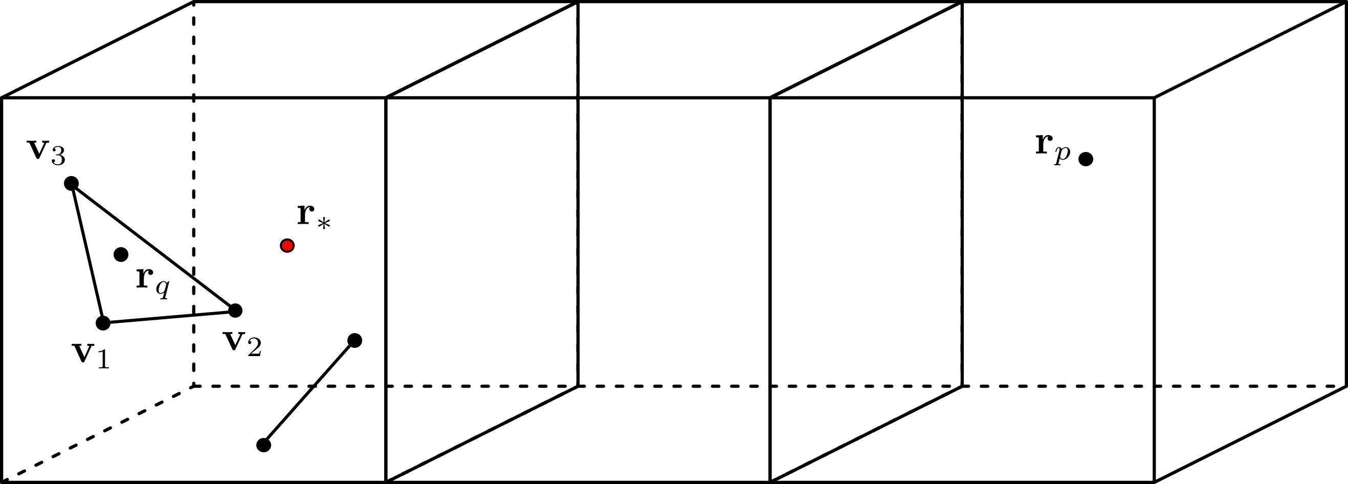
Recently, Gumerov et al. introduced Quadrature to Expansion (Q2X), a recursive method for the analytical evaluation of integrals of spherical basis functions for the Laplace equation in ${\mathbb{R}}^{3}$, aka solid harmonics, over $d$-simplex elements for $d\in\{1,2,3\}$ with constant densities [1]. This method achieves exact integration of all bases up to truncation degree $p_{\mathrm{s}}$ with optimal complexity $O(p_{\mathrm{s}}^{2})$ per element for any $d$ in $\{1,2,3\}$. This is useful for the Boundary Element Method (BEM) [2] coupled with the Fast Multipole Method (FMM) [3]. The conventional FMM performs an approximate summation of monopoles and dipoles centered at points $\mathbf{r}_{q}$ distributed in space, by expanding them into truncated multipole expansions centered at points $\mathbf{r}_{p}$. Many such expansions are consolidated into one to achieve efficiency. In the Q2X approach, recently introduced by Gumerov et al. [1], surface layer potential integrals over a surface or a line discretized via simplices were represented as such expansions, with the expansion coefficients, obtained by quadrature over the simplex, evaluated analytically via an optimal recursive procedure. Fig. 1 shows the geometrical relation of the elements with respect to the expansion center $\mathbf{r}_{*}$ of the solid harmonics, which is typically the centroid of a cell in an octree data structure to which the elements belong. Recursive analytical methods for high order surface elements have been developed for the close evaluation of layer potential integrals [4], and such a method is also desired for the integration of regular solid harmonics commonly arising in the FMM-BEM. [5] discusses a related method for quadrilateral elements, however a full algorithm for computing integrals for all harmonics and all monomial densities with finite degrees has not been described. Here, we extend the Q2X method to elements with polynomial densities which allows the evaluation of integrals for all regular solid harmonics up to degree $p_{\mathrm{s}}$ and all monomial density functions up to degree $p_{\mathrm{d}}$ with optimal complexity $O(p_{\mathrm{s}}^{2}p_{\mathrm{d}}^{d})$ per element. All formulation is done for ${\mathbb{R}}^{3}$.

The BEM is widely used for numerical solution of partial differential equations, e.g. the Poisson equation:

with field $u$ in domain $\Omega\subset{\mathbb{R}}^{3}$, and source $f$ ($=0$ for Laplace). The weak form of 1 can be written in terms of single- and double layer potentials $L$, $M$ [2]:

with $c_{p}=1/2$ on a smooth boundary, $\mathbf{n}_{q}$ the outward unit normal, $\gamma_{0}$ and $\gamma_{1}$ the boundary trace and normal derivative operators, respectively, $N_{0}$ the Newton potential operator, and $G(\mathbf{r}_{p},\mathbf{r}_{q})$ the Green function for the Laplace equation:

In the BEM the boundary $\Gamma$ is discretized into boundary elements which can be either flat or curved surfaces. The layer potential integrals over these elements are evaluated to form the linear system of equations. The densities $\sigma$ are approximated via local, typically polynomial, functions with unknown coefficients which must be determined. In the present work we assume the boundary $\Gamma=\partial\Omega$ is a union of boundary elements $\Gamma=\bigcup_{i}S_{i}$, where each $S_{i}$ is a flat triangular element with polynomial density functions.

Similarly, in vortex methods the Bio-Savart integral is used to compute potentials due to line elements $\Lambda_{q}$:

where $\mathbf{I}_{q}$ is the circulation of the $q$-th line element.

For $d=2$, we denote the vertices of the 2-simplex element as $\{\mathbf{v}_{1},\mathbf{v}_{2},\mathbf{v}_{3}\}$ and use the parametrization:

In contrast to [1] which used constant parametrization, we extend the method to density functions $\sigma$ defined over the elements which are polynomials of the form:

The integrand of the integrals $L_{n}^{m},M_{n}^{m}$ have the form:

We set the origin of the coordinate system so that $\mathbf{r}_{\ast}=\mathbf{0}$. The goal is to derive an algorithm for efficient analytical evaluation of integrals 16 for $\sigma=N_{b}^{c}(u,v)$:

for all index tuples $(n,m,b,c)$ satisfying $0\leq n\leq p_{\mathrm{s}}$, $|m|\leq n$, $0\leq b$, $0\leq c$, and $b+c\leq p_{\mathrm{d}}$. The coefficients $K_{n,b}^{m}$ for the case $d=1$ can be expressed by setting $c=0$, $\mathbf{r}_{q}=\mathbf{r}_{u}u+\mathbf{v}_{1}$, and replacing $S_{q}$ by $\Lambda_{q}$ in $L_{n,b}^{m,c}$.

We first describe the case $d=2$. The Q2X method [1] was derived by utilizing the fact that the regular spherical basis functions $R_{n}^{m}$ are homogeneous polynomials of degree $n$ of arguments $(x,y,z)$. Similarly, $N_{b}^{c}$ are also homogeneous polynomials of $(u,v)$ with degree $b+c$. Hence, by considering $\mathbf{r}$ and $(u,v)$ as functions of $(\xi,\eta,z)$, Euler’s homogeneous function theorem gives:

With $a_{s,t}$ the $(s,t)$ entry of $A^{-1}$, $\alpha_{s}^{(\pm)}\equiv a_{s,1}\pm ia_{s,2}$, $\mathbf{a}_{s}$ the $s$-th row of $A^{-1}$, and $\beta_{s}\equiv\mathbf{a}_{s}\cdot\mathbf{v}_{1}$ we obtain:

We define $\xi=\xi_{u}u+\xi_{v}v+\xi_{0}$, $\eta=\eta_{u}u+\eta_{v}v+\eta_{0}$, and $z=z_{u}u+z_{v}v+z_{0}$, where the subscripts $u$ and $v$ denote partial derivatives with respect to these variables, and

Q2XP was tested for the case $d=2$ on a configuration given by: $\mathbf{r}_{c}=\left(\sqrt{3}/2,0,0\right)^{T}$, $\mathbf{v}_{1}=\mathbf{r}_{c}+r_{t}\left(1,0,0\right)^{T}$, $\mathbf{v}_{2,3}=\mathbf{r}_{c}+r_{t}\left(-1/2,\pm\sqrt{3}/2,0\right)^{T}$, and $r_{t}=0.1$. The wall clock times for running a Python implementation of Q2XP for polynomial degrees of up to $p_{\mathrm{s}}=p_{\mathrm{d}}=20$ are shown in Fig. 2. Given a complexity expression $t=Cp_{\mathrm{s}}^{\alpha}p_{\mathrm{d}}^{\beta}$ with $t$ the computation time and $C$ a constant, the exponents are extracted as $\alpha=1.75$ and $\beta=1.83$ from the numerical experiment.

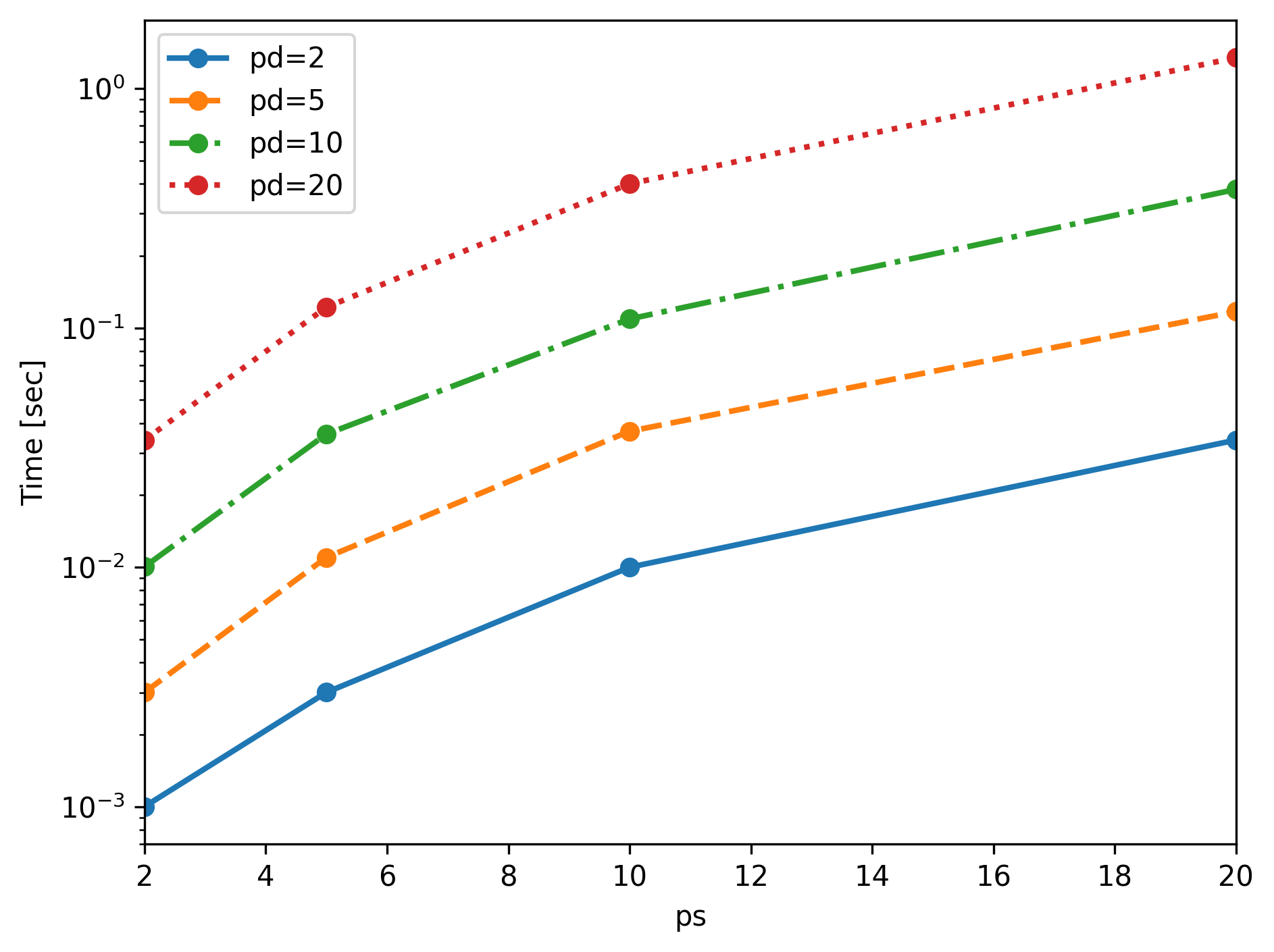
The maximum relative difference over the $L_{n,b}^{m,c}$ and $M_{n,b}^{m,c}$ coefficients for truncation degrees $p_{\mathrm{s}}=p_{\mathrm{d}}=10$ computed by exact Gauss-Legendre quadrature and Q2XP was $2.7\times 10^{-14}$, indicating good accuracy.

We have extended the recursive algorithm presented in [1] for the analytical evaluation of integrals of spherical basis functions over high order $d$-simplex elements arising in the FMM-BEM for the Laplace equation in ${\mathbb{R}}^{3}$ to the case of polynomial density functions. All multipole expansion coefficients are evaluated analytically up to spherical basis degree of $p_{\mathrm{s}}$ and the density’s polynomial degree of $p_{\mathrm{d}}$ with optimal complexity $O(p_{\mathrm{s}}^{2}p_{\mathrm{d}}^{d})$. This complexity was confirmed via numerical experiments. While we limited the discussion to $d\in\{1,2\}$, the case $d=3$ could also be supported by following the formulation presented here and in [1].

This work is supported by Cooperative Research Agreement W911NF2020213 between the University of Maryland and the Army Research Laboratory, with David Hull and Steven Vinci as Technical monitors. Shoken Kaneko thanks Japan Student Services Organization and Watanabe Foundation for scholarships.

References

• [1] Nail A Gumerov, Shoken Kaneko, and Ramani Duraiswami. Recursive Computation of the Multipole Expansions of Layer Potential Integrals over Simplices for Efficient Fast Multipole Accelerated Boundary Elements. Journal of Computational Physics, 486(1):112118, 2023.
• [2] Stefan A Sauter and Christoph Schwab. Boundary element methods. In Boundary Element Methods, pages 183–287. Springer, 2010.
• [3] Leslie Greengard and Vladimir Rokhlin. A fast algorithm for particle simulations. Journal of computational physics, 73(2):325–348, 1987.
• [4] Shoken Kaneko, Nail A Gumerov, and Ramani Duraiswami. Recursive Analytical Quadrature of Laplace and Helmholtz Layer Potentials in 3\mathbb{R}^{3}. arXiv preprint arXiv:2302.02196, 2023.
• [5] John Nicholas Newman. Distributions of sources and normal dipoles over a quadrilateral panel. Journal of Engineering Mathematics, 20(2):113–126, 1986.
• [6] Milton Abramowitz, Irene A Stegun, and Robert H Romer. Handbook of mathematical functions with formulas, graphs, and mathematical tables, volume 56. Americal Journal of Physics, 1988.
• [7] Nail A. Gumerov and Ramani Duraiswami. Fast multipole method for the biharmonic equation in three dimensions. Journal of Computational Physics, 215(1):363–383, 2006.