Efficient Quantum Walk on a Quantum Processor
Abstract
The random walk formalism is used across a wide range of applications, from modelling share prices to predicting population genetics. Likewise quantum walks have shown much potential as a framework for developing new quantum algorithms. In this paper, we present explicit efficient quantum circuits for implementing continuous-time quantum walks on the circulant class of graphs. These circuits allow us to sample from the output probability distributions of quantum walks on circulant graphs efficiently. We also show that solving the same sampling problem for arbitrary circulant quantum circuits is intractable for a classical computer, assuming conjectures from computational complexity theory. This is a new link between continuous-time quantum walks and computational complexity theory and it indicates a family of tasks which could ultimately demonstrate quantum supremacy over classical computers. As a proof of principle we have experimentally implemented the proposed quantum circuit on an example circulant graph using a two-qubit photonics quantum processor.
Quantum walks are the quantum mechanical analogue to the well-known classical random walk and they have established roles in quantum information processing farhi1998quantum ; kempe2003quantum ; childs2013universal . In particular, they are central to quantum algorithms created to tackle database search childs2004spatial , graph isomorphism douglas2008 ; gamble2010two ; berry2011 , network analysis and navigation Berry2010 ; sanchez2012quantum , and quantum simulation lloyd1996universal ; berry2012black ; schreiber20122d , as well as modelling biological processes engel2007evidence ; rebentrost2009environment . Meanwhile, physical properties of quantum walks have been demonstrated in a variety of systems, such as nuclear magnetic resonance du2003experimental ; ryan2005experimental , bulk do2005experimental and fiber schreiber2010photons optics, trapped ions xue2009quantum ; schmitz2009quantum ; zahringer2010realization , trapped neutral atoms karski2009quantum , and photonics perets2008realization ; carolan2014experimental . Almost all physical implementations of quantum walk so far followed an analog approach as for quantum simulation qwbook2014 ; qubitImplementationQW , whereby the apparatus is dedicated to implement specific instances of Hamiltonians without translation onto quantum logic. However, there is no existing method to implement analog quantum simulations with error correction or fault tolerance, and they do not scale efficiently in resources when simulating broad classes of large graphs.
In this paper, we present efficient quantum circuits for implementing continuous time quantum walks (CTQWs) on circulant graphs with an eigenvalue spectrum that can be classically computed efficiently. These quantum circuits provide the time-evolution states of CTQWs on circulant graphs exponentially faster than best previously known methods ng2004iterative . We report a proof-of-principle experiment, where we implement CTQWs on an example circulant graph (namely the complete graph of four vertices) using a two-qubit photonics quantum processor to sample the probability distributions and perform state tomography on the output state of a CTQW. We also provide evidence from computational complexity theory that the probability distributions that are output from the circuits of this circulant form are hard to sample from using a classical computer, implying our scheme also provides an exponential speedup for sampling.
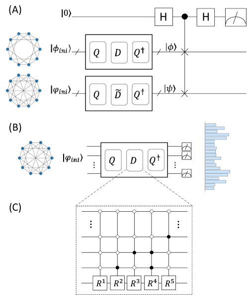
Efficient quantum circuit implementations of CTQWs have been presented for sparse and efficiently row-computable graphs aharonov2003adiabatic ; berry2007efficient , and specific non-sparse graphs childs2009limitations ; childs2010relationship . However, the design of quantum circuits for implementing CTQWs is in general difficult, since the time-evolution operator is time-dependent and non-local farhi1998quantum . A subset of circulant graphs have the property that their eigenvalues and eigenvectors can be classically computed efficiently gray2006toeplitz ; ng2004iterative . This enables us to construct a scheme that efficiently outputs the quantum state , which corresponds to the time evolution state of a CTQW on corresponding graphs. One can then either perform direct measurements on or implement further quantum circuit operations to extract physically meaningful information. For example the “SWAP test” buhrman2001quantum can be used to estimate the similarity of dynamical behaviors of two circulant Hamiltonians operating on two different initial states, as shown in Figure 1(A). This procedure can also be adapted to study the stability of quantum dynamics of circulant molecules (for example, the DNA Möbius strips han2010folding ) in a perturbational environment peres1984stability ; prosen2002stability .
On the other hand, when measuring in the computational basis we can sample the probability distribution
| (1) |
that describes the probability of observing the quantum walker at position —an -bit string, corresponding to the vertices of the given graph, as shown in Figure 1(B). Sampling of this form is sufficient to solve various search and characterization problems childs2004spatial ; sanchez2012quantum , and can be used to deduce critical parameters of the quantum walk, such as mixing time kempe2003quantum . It is unlikely for a classical computer to be able to efficiently sample from . We adapt the similar methodology of refs. aaronson2011computational ; bremner2010classical ; bremner2015average to show that if there did exist a classical sampler for a somewhat more general class of circuits, this would have the following unlikely complexity-theoretic implication: the infinite tower of complexity classes known as the polynomial hierarchy would collapse. This evidence of hardness exists despite the classical efficiency with which properties of the CTQW, such as the eigenvalues of circulant graphs, can be computed on a classical machine.
For an undirected graph of vertices, a quantum particle (or “quantum walker”) placed on evolves into a superposition of states in the orthonormal basis that correspond to vertices of . The exact evolution of the CTQW is governed by connections between the vertices of : where the Hamiltonian is given by for hopping rate per edge per unit time and where is the -by- symmetric adjacency matrix, whose entries are , if vertices and are connected by an edge in , and otherwise farhi1998quantum .
Circulant graphs are defined by symmetric circulant adjacency matrices for which each row when right-rotated by one element, equals the next row —for example complete graphs, cycle graphs and Mobius ladder graphs are all subclasses of circulant graphs. It follows that Hamiltonians for CTQWs on any circulant graph have a symmetric circulant matrix representation, which can be diagonalized by the unitary Fourier transform gray2006toeplitz , i.e. , where
| (2) |
and is a diagonal matrix containing eigenvalues of , which are all real and whose order is determined by the order of the eigenvectors in . Consequently, we have , where the time dependence of is confined to the diagonal unitary operator .
The Fourier transformation can be implemented efficiently by the well-known QFT quantum circuit nielsen2010quantum . For a circulant graph that has vertices, the required QFT of dimension can be implemented with quantum gates acting on qubits. To implement the inverse QFT, the same circuit is used in reverse order with phase gates of opposite sign. can be implemented using at most controlled-phase gates with phase values being a linear function of , because an arbitrary phase can be applied to an arbitrary basis state, conditional on at most qubits. Given a circulant graph that has non-zero eigenvalues, only controlled-phase gates are needed to implement . If the given circulant graph has distinct eigenvalues, which can be characterised efficiently (such as the cycle graphs and Mobius ladder graphs), we are still able to implement the diagonal unitary operator using polynomial quantum resources. A general construction of efficient quantum circuits for was given by Childs childs2004quantum , and is shown in the Appendix for completeness. Thus, the quantum circuit implementations of CTQWs on circulant graphs can be constructed, which have an overall complexity of , and act on at most qubits. Compared with the best known classical algorithm based on fast Fourier transform, that has the computational complexity of ng2004iterative , the proposed quantum circuit implementation generates the evolution state with an exponential advantage in speed.
Consider a circuit of the form , where is a diagonal matrix made up of controlled-phase gates. Define
| (3) |
represents a family of circuits having the following structure: each qubit line begins and ends with a Hadamard () gate, and, in between, every gate is diagonal in the computational basis. This class of circuits is known as instantaneous quantum polynomial time (IQP) shepherd2009temporally ; bremner2010classical . It is known that computing for arbitrary diagonal unitaries made up of circuits of gates, even if each acts on qubits, is #P-hard bremner2015average ; fujii13 ; goldberg14 . This hardness result even holds for approximating up to any multiplicative error strictly less than fujii13 ; goldberg14 , where is said to approximate up to multiplicative error if
| (4) |
Towards a contradiction, assume that there exists a polynomial-time randomized classical algorithm which samples from . Then a classic result of Stockmeyer stockmeyer1985on states that there is an algorithm in the complexity class FBPP which can approximate any desired probability to within multiplicative error . This complexity class FBPP—described as polynomial-time randomized classical computation equipped with an oracle to solve arbitrary NP problems—sits within the infinite tower of complexity classes known as the polynomial(-time) hierarchy papadimitriou1994computational . Combining with the above hardness result of approximating , we find that the assumption implies that an FBPP algorithm solves a #P-hard problem, so P would be contained within FBPP, and therefore the polynomial hierarchy would collapse to its third level. This consequence is considered very unlikely in computational complexity theory papadimitriou1994computational .
We therefore conclude that a polynomial-time randomized classical sampler from the distribution is unlikely to exist. Further, this even holds for classical algorithms which sample from any distribution which approximates up to multiplicative error strictly less than in each probability . It is worth noting that if the output distribution results from measurements on only qubits van2011simulating , or obeys the sparsity promise that only a -sized, and a priori unknown, subset of the measurement probabilities are nonzero schwarz2013simulating , it could be classically efficiently sampled. The proof of hardness here does not hold for the approximate sampling from up to small additive error. It is an interesting open question whether similar techniques to aaronson2011computational ; bremner2015average can be used to prove hardness of the approximate case, perhaps conditioned on other conjectures in complexity theory.
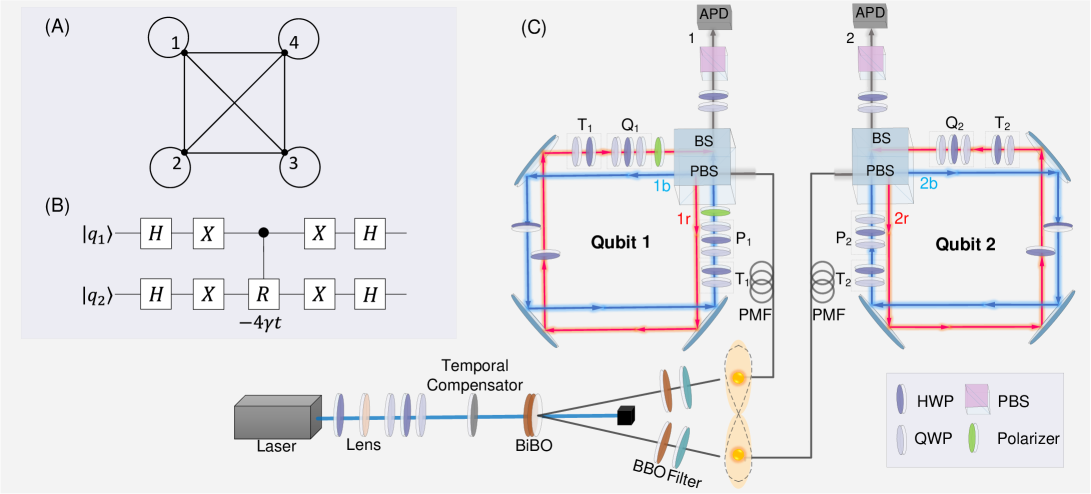
As an experimental demonstration, we used a photonic quantum logic to simulate CTQWs on the graph—a complete graph with self loops on four vertices (Figure 2(A)). Complete graphs are a special kind of circulant graph, with an adjacency matrix where for all . The Hamiltonian of a complete graph on vertices has only 2 distinct eigenvalues, 0 and . Therefore, the diagonal matrix of eigenvalues of is . Following the aforementioned discussion, we can readily construct the quantum circuit for implementing CTQWs on graph based on diagonalization using the QFT matrix. However, the choice of using the QFT matrix as the eigenbasis of Hamiltonian is not strictly necessary – any equivalent eigenbasis can be selected. Through the diagonalization using Hadamard eigenbasis, an alternative efficient quantum circuit for implementing CTQWs on graph is shown in Figure 2(B), which can be easily extended to the complete graph on vertices.
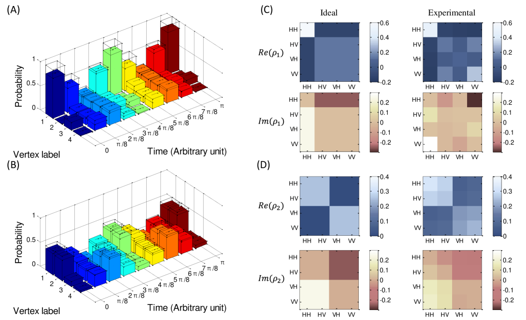
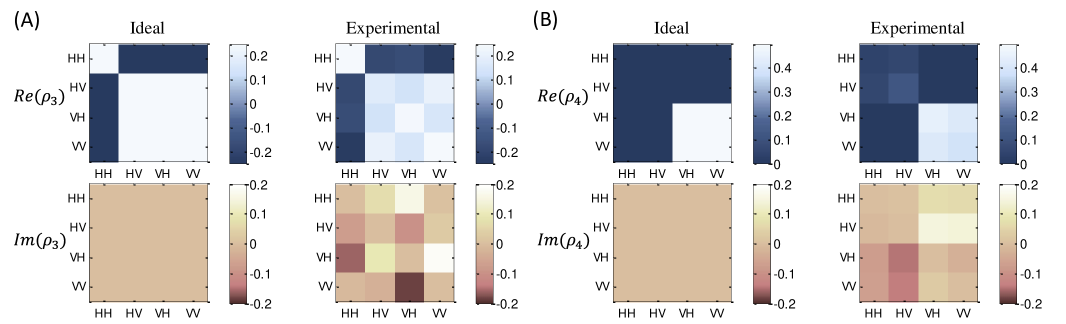
We built a configurable two-qubit photonics quantum processor (Figure 2(C)), adapting the entanglement-based technique presented in zhou2011adding , and implemented CTQWs on graph with various evolving times and initial states. Specifically, we prepared two different initial states and , which represent the quantum walker starting from vertex 1, and the superposition of vertices 1 and 2 respectively. We chose the evolution time following the list , which covers the whole periodical characteristics of CTQWs on graph. For each evolution, we sampled the corresponding probability distribution with fixed integration time, shown in Figure 3(A) and (B). To measure how close the experimental and ideal probability distributions are, we calculated the average fidelities defined as . The achieved average fidelities for the samplings with two distinct initial states are 96.680.27% and 95.820.25% respectively. Through the proposed circuit implementation, we are also able to examine the evolution states using quantum state tomography, which is generally difficult for the analog simulations. For two specific evolution states and , we performed quantum state tomography and reconstructed the density matrices using the maximum likelihood estimation technique. The two reconstructed density matrices achieve fidelities of 85.811.08% and 88.440.97% respectively, shown in Figure 3(C) and (D).
In this paper, we have described how CTQWs on circulant graphs can be efficiently implemented on a quantum computer, if the eigenvalues of the graphs can be characterised efficiently classically. In fact, we can construct an efficient quantum circuit to implement CTQWs on any graph whose adjacency matrix is efficiently diagonalisable, in other words, as long as the matrix of column eigenvectors and the diagonal matrix of the eigenvalue exponentials can be implemented efficiently. We have shown that the problem of sampling from the output probability distributions of quantum circuits of the form is hard for classical computers, based on a highly plausible conjecture that the polynomial hierarchy does not collapse. This observation is particularly interesting from both perspectives of CTQW and computational complexity theory, as it provides new insights into the CTQW framework and also helps to classify and identify new problems in computational complexity theory. For the CTQWs on the circulant graphs of non-zero eigenvalues, the proposed quantum circuit implementations do not need a fully universal quantum computer, and thus can be viewed as an intermediate model of quantum computation. Although the hardness of the approximate case of the sampling problem is unknown, the evidence we provided for the exact case indicates a promising candidate for experimentally establishing quantum supremacy over classical computers, and further evidence against the extended Church-Turing thesis. Compared with other intermediate models such as the one clean qubit model knill1998power , IQP and boson sampling aaronson2011computational , the quantum circuit implementation of CTQWs is also more appealing due to available methods in fault tolerance and error correction, which are difficult to implement for other models rohde2012error . This may also lead onto other practical applications through the use of CTQWs for quantum algorithm design.
Experimental Setup A diagonally polarized, 120 mW, continuous-wave laser beam with central wavelength of 404 nm is focused at the centre of paired type-I BiBO crystals with their optical axes orthogonally aligned to each other, to create the polarization entangled photon-pairs rangarajan2009optimizing . Through the spontaneous parametric down-conversion process, the photon pairs are generated in the state of , where and represent horizontal and vertical polarization respectively. The photons pass through the polarization beam-splitter (PBS) part of the dual PBS/beam-splitter (BS) cubes on both arms to generate two-photon four-mode state of the form ( and label red and blue paths shown in Figure 2(C)). Rotations and on each path, consisting of half wave-plate (HWP) and quarter wave-plate (QWP), convert the state into , where and can be arbitrary single-qubit states. The four spatial modes , , and pass through four single-qubit quantum gates , , and respectively, where each of the four gates is implemented through three wave plates: QWP, HWP and QWP. The spatial modes and ( and ) are then mixed on the BS part of the cube. By post-selecting the case where the two photons exit at ports 1 and 2, we obtain the state . In this way, we implement a two-qubit quantum operation of the form on the initialized state .
As shown in Figure 2(B), the quantum circuit for implementing CTQW on the graph consists of Hadamard gates (H), Pauli-X gates (X) and controlled-phase gate (CP). CP is implemented by configuring , , , , where and are implemented by polarizers. Together with combining the operation before CP with state preparation and the operation after CP with measurement setting, we implement the whole quantum circuit on the experimental setup. The evolution time of CTQW is controlled by the phase value of , which is determined by setting the three wave plates of in Figure 2(C) to QWP(), HWP(), QWP(), where the angle of HWP equals to the phase of . The evolution time is then given by
Acknowledgements.
References
- (1) Farhi, E. & Gutmann, S. Quantum computation and decision trees. Phys. Rev. A 58, 915 (1998).
- (2) Kempe, J. Quantum random walks: an introductory overview. Contemp. Phys. 44, 307-327 (2003).
- (3) Childs, A. M., Gosset, D. & Webb, Z. Universal computation by multiparticle quantum walk. Science 339, 791-794 (2013).
- (4) Childs, A. M. & Goldstone, J. Spatial search by quantum walk. Phys. Rev. A 70, 022314 (2004).
- (5) Douglas, B. L. & Wang, J. B. A classical approach to the graph isomorphism problem using quantum walks. J. Phys. A 41, 075303 (2008).
- (6) Gamble, J. K., Friesen, M., Zhou, D., Joynt, R. & Coppersmith, S. N. Two-particle quantum walks applied to the graph isomorphism problem. Phys. Rev. A 81, 052313 (2010).
- (7) Berry, S. D. & Wang, J. B. Two-particle quantum walks: Entanglement and graph isomorphism testing. Phys. Rev. A 83, 042317 (2011).
- (8) Berry, S. D. & Wang, J. B. Quantum-walk-based search and centrality. Phys. Rev. A 82, 042333 (2010).
- (9) Sánchez-Burillo, E., Duch, J., Gómez-Gardeñes, J. & Zueco, D. Quantum navigation and ranking in complex networks. Sci. Rep. 2, 605 (2012).
- (10) Lloyd, S. Universal quantum simulators. Science 273, 1073-1078 (1996).
- (11) Berry, D. W. & Childs, A. M. Black-box hamiltonian simulation and unitary implementation. Quantum Inf. Comput. 12, 29-62 (2012).
- (12) Schreiber, A. et al. A 2D quantum walk simulation of two-particle dynamics. Science 336, 55-58 (2012).
- (13) Engel, G. S. et al. Evidence for wavelike energy transfer through quantum coherence in photosynthetic systems. Nature 446, 782-786 (2007).
- (14) Rebentrost, P. et al. Environment-assisted quantum transport. New J. Phys. 11, 033003 (2009).
- (15) Du, J. et al. Experimental implementation of the quantum random-walk algorithm. Phys. Rev. A 67, 042316 (2003).
- (16) Ryan, C. A. et al. Experimental implementation of a discrete-time quantum random walk on an NMR quantum-information processor. Phys. Rev. A 72, 062317 (2005).
- (17) Do, B. et al. Experimental realization of a quantum quincunx by use of linear optical elements. J. Opt. Soc. Am. B 22, 499-504 (2005).
- (18) Schreiber, A. et al. Photons walking the line: a quantum walk with adjustable coin operations. Phys. Rev. Lett. 104, 050502 (2010).
- (19) Xue, P., Sanders, B. C. & Leibfried, D. Quantum walk on a line for a trapped ion. Phys. Rev. Lett. 103, 183602 (2009).
- (20) Schmitz, H. et al. Quantum walk of a trapped ion in phase space. Phys. Rev. Lett. 103, 090504 (2009).
- (21) Zähringer, F. et al. Realization of a quantum walk with one and two trapped ions. Phys. Rev. Lett. 104, 100503 (2010).
- (22) Karski, M. et al. Quantum walk in position space with single optically trapped atoms. Science 325, 174-177 (2009).
- (23) Perets, H. B. et al. Realization of quantum walks with negligible decoherence in waveguide lattices. Phys. Rev. Lett. 100, 170506 (2008).
- (24) Carolan, J. et al. On the experimental verification of quantum complexity in linear optics. Nat. Photonics 8, 621 (2014).
- (25) Manouchehri, K. & Wang, J. B. Physical Implementation of Quantum Walks. Springer-Verlag, Berlin, (2014).
- (26) Exceptions, such as du2003experimental , adopted the qubit model, but there was no discussion on potentially efficient implementation of quantum walks.
- (27) Ng, M. K. Iterative Methods for Toeplitz Systems. Oxford University Press New York, (2004).
- (28) Aharonov, D. & Ta-Shma, A. Adiabatic quantum state generation and statistical zero knowledge. In Proceedings of the thirty-fifth annual ACM symposium on Theory of computing 20-29. ACM (2003).
- (29) Berry, D. W., Ahokas, G., Cleve, R. & Sanders, B. C. Efficient quantum algorithms for simulating sparse hamiltonians. Commun. Math. Phys. 270, 359-371 (2007).
- (30) Childs, A. M. & Kothari, R. Limitations on the simulation of non-sparse hamiltonians. Quantum Inf. Comput. 10, 669-684 (2009).
- (31) Childs, A. M. On the relationship between continuous-and discrete-time quantum walk. Commun. Math. Phys. 294, 581-603 (2010).
- (32) Gray, R. M. Toeplitz and Circulant Matrices: A Review. Now Publishers Inc., (2006).
- (33) Buhrman, H., Cleve, R., Watrous, J. & De Wolf, R. Quantum fingerprinting. Phys. Rev. Lett. 87, 167902 (2001).
- (34) Han, D. et al. Folding and cutting DNA into reconfigurable topological nanostructures. Nat. Nanotechnol 5, 712-717 (2010).
- (35) Peres, A. Stability of quantum motion in chaotic and regular systems. Phys. Rev. A 30, 1610 (1984).
- (36) Prosen, T. & Znidaric, M. Stability of quantum motion and correlation decay. J. Phys. A: Math. Gen. 35, 1455 (2002).
- (37) Aaronson, S. & Arkhipov, A. The computational complexity of linear optics. In Proceedings of the forty-third annual ACM symposium on Theory of computing 333–342. ACM (2011).
- (38) Bremner, M. J., Jozsa, R. & Shepherd, D. J. Classical simulation of commuting quantum computations implies collapse of the polynomial hierarchy. Proceedings of the Royal Society A: Mathematical, Physical and Engineering Science, rspa.2010.0301 (2010).
- (39) Bremner, M. J., Montanaro, A. & Shepherd, D. J. Average-case complexity versus approximate simulation of commuting quantum computations, Preprint at http://arxiv.org/abs/1504.07999 (2015).
- (40) Nielsen, N. A. & Chuang, I. L. Quantum Computation and Quantum Information. Cambridge University Press, (2010).
- (41) Childs, A. M. Quantum information processing in continuous time. PhD Thesis, Massachusetts Institute of Technology (2004).
- (42) Shepherd, D. & Bremner, M. J. Temporally unstructured quantum computation. Proceedings of the Royal Society A: Mathematical, Physical and Engineering Science 465, 1413-1439 (2009).
- (43) Fujii, K. & Morimae, T. Quantum commuting circuits and complexity of Ising partition functions, Preprint at http://arxiv.org/abs/1311.2128 (2013).
- (44) Goldberg, L. A. & Guo, H. The complexity of approximating complex-valued Ising and Tutte partition functions, Preprint at http://arxiv.org/abs/1409.5627 (2014).
- (45) Stockmeyer, L. J. On approximation algorithms for #P. SIAM J. Comput. 14, 849-861 (1985).
- (46) Papadimitriou, C. Computational Complexity. Addison-Wesley, (1994).
- (47) Nest, M. Simulating quantum computers with probabilistic methods. Quantum Inf. Comput. 11, 784-812 (2011).
- (48) Schwarz, M. & Nest, M. Simulating quantum circuits with sparse output distributions, Preprint at http://arxiv.org/abs/1310.6749 (2013).
- (49) Zhou, X. Q. et al. Adding control to arbitrary unknown quantum operations. Nat. Commun. 2, 413 (2011).
- (50) Knill, E., & Laflamme, R. Power of one bit of quantum information. Phys. Rev. Lett. 81, 5672 (1998).
- (51) Rohde, P. P. & Ralph, T. C. Error tolerance of the boson-sampling model for linear optics quantum computing. Phys. Rev. A 85, 022332 (2012).
- (52) Rangarajan, R., Goggin, M. & Kwiat, P. Optimizing type-I polarization-entangled photons. Opt. Express 17, 18920-18933 (2009).
Appendix
I Further Details on Circulant Graphs and Other Examples
A circulant graph of vertices is fully described by an -by- symmetric circulant adjacency matrix defined as follows.
| (A6) |
where . Obviously, every circulant matrix can be generated given any row of the matrix – conventionally we use the first row of the matrix, denoted as . It is clear that has at most distinct eigenvalues which are given by , where and ng2004iterative_appendix . If is singular, some of the eigenvalues of are zeros. The complete graph and complete bipartite graph are straightforward examples of circulant graphs with few distinct eigenvalues.
There are also some other interesting examples of circulant graph such as self-complementary circulant graphs and Paley graphs with prime order zhou2011self ; rajasingh2013spanning . Both of these two families of graphs are also strongly regular graphs which have only three distinct eigenvalues. For example, the Paley graph on 13 vertices has three distinct eigenvalues: 6 (with multiplicity 1) and (both with multiplicity 6), and thus the diagonal unitary can be implemented efficiently. We note here it is required to implement QFT (and its inverse) for the dimension of 13, which does not have the form of . The QFT on general dimensions can be implemented by means of amplitude amplification with extra qubit registers to perform the computation mosca2004exact . Alternatively, approximate versions of the QFT on general dimensions have also been developed hales2000improved .
II Implementation of the Diagonal Unitary Operator
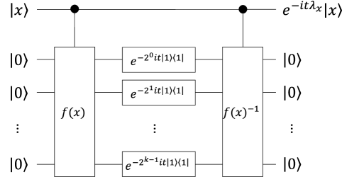
We say that the eigenvalues of a circulant graph can be characterised efficiently, if they can be calculated efficiently classically. In other words, the eigenvalue matrix of the given circulant Hamiltonian can be efficiently computed, and thus the diagonal unitary operator can be efficiently implemented childs2004quantum . Specifically, there exists a quantum circuit shown in Figure A1, which transforms a computational basis state , together with a -qubit ancilla for , as
| (A7) |
where . Note that here we assume can be expressed exactly as a rational number with bits of precision. If this is not the case, truncating to bits of precision will introduce an error which can be made arbitrarily small by taking large enough . The function returns for any given . is always a real number since the adjacency matrix is symmetric.
For example, for the case of the cycle graph of vertices, there are essentially distinct eigenvalues simply given by , where . And then will be the cosine function that can be computed with a number of operations polynomial in , using a reversible equivalent of classical algorithms to compute trigonometric functions, e.g. the Taylor approximation. In general, given a sparse circulant graph which has only s in the first row of its adjacency matrix, an efficient function can be given as
| (A8) |
where is the set of positions for which the first row in nonzero. is a sum of numbers, taking time to compute. For a non-sparse circulant graph, its eigenvalues are still possible to be calculated efficiently classically. Some straightforward examples are complete graph, complete bipartite graph and cocktail party graph. Therefore, together with the quantum circuits of QFT and the inverse of QFT, we construct an efficient quantum circuit for implementing CTQW on the circulant graph whose eigenvalues can be computed efficiently classically.
III Complexity Analysis of “SWAP test”
Unlike the sampling problem we discussed in the main text, the scenario of “SWAP test”, where we compare two unitary processes and , could sometimes be easier for a classical computer. Imagine we start each process in the state . Then the overlap between the resulting output states approximated by the SWAP test satisfies
| (A9) |
where is the value at position on the diagonal of . can be approximated by a classical algorithm up to additive error. The algorithm simply takes the average of values of the product for uniformly random . For each , this value can be computed exactly in polynomial time.
This highlights that the complexity of comparing and depends on the choice of input states and . In full generality, one could allow these to be arbitrary states produced by a polynomial-time quantum computation; the state comparison problem would then be BQP-complete, but for rather trivial reasons. We expect that the problem would remain classically hard for choices of initial states relevant, for example, to quantum-chemistry applications. On the other hand, the SWAP test can still be used as in Scenario (B) in the main text to compare the evolution of two Hamiltonians, one of which is not circulant but is efficiently implementable. In this case, the comparison problem is also BQP-complete, and hence expected to be hard for a classical computer.
IV Further Experimental Results
We present the ideal and experimentally sampled probability distributions of CTQW with initial states , (mentioned in the main text), , , , , in Table I. The achieved average fidelities between ideal and experimental probability distributions are 96.680.27%, 95.820.25%, 92.610.21%, 96.360.16%, 98.760.17% and 97.270.24% respectively. In the main text, we reconstructed the density matrices for the two quantum states and , through performing quantum state tomography. Here we also present the reconstructed density matrices for another two evolution states and , with the achieved fidelities of 88.631.24% and 91.530.53% respectively. See in Figure A2. The four reconstructed density matrices , , and for quantum states , , and are shown as follows.
| Node/T | 0 | ||||||||
|---|---|---|---|---|---|---|---|---|---|
| 1 | 0.625 | 0.25 | 0.625 | 1 | 0.625 | 0.25 | 0.625 | 1 | |
| 0 | 0.125 | 0.25 | 0.125 | 0 | 0.125 | 0.25 | 0.125 | 0 | |
| 0 | 0.125 | 0.25 | 0.125 | 0 | 0.125 | 0.25 | 0.125 | 0 | |
| 0 | 0.125 | 0.25 | 0.125 | 0 | 0.125 | 0.25 | 0.125 | 0 | |
| 0.8225 | 0.5014 | 0.2139 | 0.5759 | 0.8482 | 0.4583 | 0.2414 | 0.549 | 0.858 | |
| 0.003 | 0.1388 | 0.2254 | 0.1455 | 0.0078 | 0.2167 | 0.2375 | 0.1324 | 0.0114 | |
| 0.1598 | 0.153 | 0.2659 | 0.2105 | 0.1284 | 0.1333 | 0.2299 | 0.1912 | 0.1193 | |
| 0.0148 | 0.2068 | 0.2948 | 0.0681 | 0.0156 | 0.1917 | 0.2912 | 0.1275 | 0.0114 |
| Node/T | 0 | ||||||||
|---|---|---|---|---|---|---|---|---|---|
| 0.5 | 0.25 | 0 | 0.25 | 0.5 | 0.25 | 0 | 0.25 | 0.5 | |
| 0.5 | 0.25 | 0 | 0.25 | 0.5 | 0.25 | 0 | 0.25 | 0.5 | |
| 0 | 0.25 | 0.5 | 0.25 | 0 | 0.25 | 0.5 | 0.25 | 0 | |
| 0 | 0.25 | 0.5 | 0.25 | 0 | 0.25 | 0.5 | 0.25 | 0 | |
| 0.4386 | 0.2796 | 0.0682 | 0.2927 | 0.4375 | 0.2823 | 0.0669 | 0.2338 | 0.434 | |
| 0.4189 | 0.2607 | 0.0746 | 0.2717 | 0.4103 | 0.3008 | 0.0605 | 0.2 | 0.4415 | |
| 0.1031 | 0.2156 | 0.3945 | 0.2482 | 0.0679 | 0.2058 | 0.4108 | 0.2923 | 0.0566 | |
| 0.0395 | 0.2441 | 0.4627 | 0.1874 | 0.0842 | 0.2111 | 0.4618 | 0.2738 | 0.0679 |
| Node/T | 0 | ||||||||
|---|---|---|---|---|---|---|---|---|---|
| 0.5 | 0.5 | 0.5 | 0.5 | 0.5 | 0.5 | 0.5 | 0.5 | 0.5 | |
| 0.5 | 0.5 | 0.5 | 0.5 | 0.5 | 0.5 | 0.5 | 0.5 | 0.5 | |
| 0 | 0 | 0 | 0 | 0 | 0 | 0 | 0 | 0 | |
| 0 | 0 | 0 | 0 | 0 | 0 | 0 | 0 | 0 | |
| 0.4147 | 0.3918 | 0.3865 | 0.4289 | 0.4156 | 0.382 | 0.4058 | 0.4356 | 0.4123 | |
| 0.4627 | 0.474 | 0.4679 | 0.4348 | 0.4359 | 0.4697 | 0.4507 | 0.4189 | 0.4416 | |
| 0.0601 | 0.0671 | 0.0722 | 0.0782 | 0.0898 | 0.0877 | 0.0792 | 0.0933 | 0.0823 | |
| 0.0625 | 0.0671 | 0.0734 | 0.0581 | 0.0587 | 0.0606 | 0.0642 | 0.0522 | 0.0639 |
| Node/T | 0 | ||||||||
|---|---|---|---|---|---|---|---|---|---|
| 0.5 | 0.125 | 0.25 | 0.625 | 0.5 | 0.125 | 0.25 | 0.625 | 0.5 | |
| 0.5 | 0.625 | 0.25 | 0.125 | 0.5 | 0.625 | 0.25 | 0.125 | 0.5 | |
| 0 | 0.125 | 0.25 | 0.125 | 0 | 0.125 | 0.25 | 0.125 | 0 | |
| 0 | 0.125 | 0.25 | 0.125 | 0 | 0.125 | 0.25 | 0.125 | 0 | |
| 0.4178 | 0.1655 | 0.1969 | 0.4932 | 0.4729 | 0.1492 | 0.1977 | 0.4217 | 0.4332 | |
| 0.3541 | 0.548 | 0.2749 | 0.1504 | 0.3824 | 0.6258 | 0.2503 | 0.1085 | 0.4308 | |
| 0.1376 | 0.1015 | 0.211 | 0.1467 | 0.0594 | 0.1047 | 0.2316 | 0.2796 | 0.0734 | |
| 0.0904 | 0.185 | 0.3171 | 0.2096 | 0.0853 | 0.1203 | 0.3205 | 0.1902 | 0.0626 |
| Node/T | 0 | ||||||||
|---|---|---|---|---|---|---|---|---|---|
| 0.25 | 0.5 | 0.25 | 0 | 0.25 | 0.5 | 0.25 | 0 | 0.25 | |
| 0.25 | 0 | 0.25 | 0.5 | 0.25 | 0 | 0.25 | 0.5 | 0.25 | |
| 0.25 | 0.5 | 0.25 | 0 | 0.25 | 0.5 | 0.25 | 0 | 0.25 | |
| 0.25 | 0 | 0.25 | 0.5 | 0.25 | 0 | 0.25 | 0.5 | 0.25 | |
| 0.2642 | 0.4163 | 0.2227 | 0.0172 | 0.2191 | 0.4136 | 0.2167 | 0.0591 | 0.2476 | |
| 0.2724 | 0.0156 | 0.3 | 0.4678 | 0.2367 | 0.0227 | 0.2808 | 0.4864 | 0.199 | |
| 0.2561 | 0.5525 | 0.2409 | 0.0043 | 0.3145 | 0.5545 | 0.2266 | 0.0227 | 0.3204 | |
| 0.2073 | 0.0156 | 0.2364 | 0.5107 | 0.2297 | 0.0091 | 0.2759 | 0.4318 | 0.233 |
| Node/T | 0 | ||||||||
|---|---|---|---|---|---|---|---|---|---|
| 0.25 | 0.625 | 0.5 | 0.125 | 0.25 | 0.625 | 0.5 | 0.125 | 0.25 | |
| 0.25 | 0.125 | 0 | 0.125 | 0.25 | 0.125 | 0 | 0.125 | 0.25 | |
| 0.25 | 0.125 | 0 | 0.125 | 0.25 | 0.125 | 0 | 0.125 | 0.25 | |
| 0.25 | 0.125 | 0.5 | 0.625 | 0.25 | 0.125 | 0.5 | 0.625 | 0.25 | |
| 0.2056 | 0.4226 | 0.3307 | 0.1129 | 0.168 | 0.4883 | 0.3425 | 0.1321 | 0.3347 | |
| 0.1542 | 0.2469 | 0.0906 | 0.0887 | 0.127 | 0.1596 | 0.0827 | 0.0566 | 0.3431 | |
| 0.2477 | 0.1674 | 0.0354 | 0.1411 | 0.3238 | 0.1643 | 0.0276 | 0.1358 | 0.1715 | |
| 0.3925 | 0.1632 | 0.5433 | 0.6573 | 0.3811 | 0.1878 | 0.5472 | 0.6755 | 0.1506 |
References
- (1) Ng, M. K. Iterative Methods for Toeplitz Systems. Oxford University Press New York, (2004).
- (2) Zhou, H. On self-complementary of circulant graphs. In Theoretical and Mathematical Foundations of Computer Science 464-471, Springer (2011).
- (3) Rajasingh, I. & Natarajan, P. Spanning trees in circulant networks. 2013.
- (4) Mosca, M. & Zalka, C. Exact quantum fourier transforms and discrete logarithm algorithms. Int. J. Quantum Inf. 2 91-100 (2004).
- (5) Hales, L. & Hallgren, S. An improved quantum fourier transform algorithm and applications. In Foundations of Computer Science, 2000. Proceedings. 41st Annual Symposium on 515-525, IEEE (2000).
- (6) Childs, A. M. Quantum information processing in continuous time. PhD Thesis, Massachusetts Institute of Technology (2004).