Efficient Relation-aware Scoring Function Search for Knowledge Graph Embedding
Abstract
The scoring function, which measures the plausibility of triplets in knowledge graphs (KGs), is the key to ensure the excellent performance of KG embedding, and its design is also an important problem in the literature. Automated machine learning (AutoML) techniques have recently been introduced into KG to design task-aware scoring functions, which achieve the state-of-the-art performance in KG embedding. However, the effectiveness of searched scoring functions is still not as good as desired. In this paper, observing that existing scoring functions can exhibit distinct performance on different semantic patterns, we are motivated to explore such semantics by searching relation-aware scoring functions. But the relation-aware search requires a much larger search space than the previous one. Hence, we propose to encode the space as a supernet and propose an efficient alternative minimization algorithm to search through the supernet in a one-shot manner. Finally, experimental results on benchmark datasets demonstrate that the proposed method can efficiently search relation-aware scoring functions, and achieve better embedding performance than state-of-the-art methods. 111The work was done when S. Di was an intern in 4Paradigm Inc. mentored by Q. Yao; and Correspondence is to Q.Yao.
Index Terms:
Knowledge Graph, Knowledge Graph Embedding, Neural Architecture Search, Automated Machine LearningI Introduction
Knowledge Graph (KG) [1, 2], as one of the most effective ways to explore and organize knowledge base, applies to various problems, such as question answering [3], recommendation [4], and few-shot learning [5]. In KGs, every edge represents a knowledge triplet in the form of (head entity, relation, tail entity), or for simplicity. Given a triplet, several crucial tasks in KGs, such as link prediction and triplet classification [1, 2], can be used to verify whether such a fact exists to form this triplet. KG embedding has been proposed to address this issue. Basically, KG embedding targets to embed entities and relations into low-dimensional vector space such as . Then based on the embeddings, a scoring function is employed to compute a score to verify whether a triplet is a fact. Triplets with higher scores are more likely to be facts.
In the last decade, various scoring functions have been proposed to significantly improve the quality of embeddings [6, 1, 2]. TransE [7], as a representative scoring function, interprets the relation as a translation from head entity to tail entity , and optimizes the embeddings to satisfy . However, TransE [7] and its variants [8, 9] are not fully expressive and their empirical performance is inferior to the others as mentioned in [10]. Recently, some works [11, 12, 13] employ neural networks to design universal scoring functions. But these scoring functions are not well-regularized for the KG properties and are expensive to general predictions [14]. Furthermore, bilinear models (BLMs) [15, 16, 17, 18, 19] are proposed to compute the score by the weighted sum of pairwise interactions of embeddings. Currently, BLMs are the most powerful in terms of both empirical results and theoretical guarantees [19] on expressiveness [10, 17].
Generally, the models in BLMs share the form as , where returns a square matrix referring to the relation . DistMult [15] regularizes to be diagonal, such as , in order to solve the overfitting problem. ComplEx [16] extends the embeddings to be complex values. SimplE [17] is another variant that regularizes the matrix with a simpler but valid constraint. More recently, TuckER [20] extends BLMs to tensor models for KG embedding. However, the designing of scoring functions is still challenging because of the diversity of KGs [2]. A scoring function performs well on one task may not adapt well to the other tasks since different KGs usually own distinct patterns [14], especially the relation patterns [2].
Recently, automated machine learning (AutoML) [21, 22], as demonstrated via automated hyperparameter tuning [23] and neural architecture search (NAS) [24], has shown to be very useful in the design of machine learning models. Inspired by such a success, a pioneered work, AutoSF [14], has proposed to search an appropriate scoring function for any given KG data using AutoML techniques. AutoSF first defines the manual scoring functions design problem as a scoring function search problem and then proposes a search algorithm. It empirically shows that the searched scoring functions are KG dependent and outperform the state-of-the-art ones designed by human experts. In short, AutoSF can search for proper scoring functions, which depend on the given KG data and evaluation metric. In other words, AutoSF is task-aware, while traditional scoring functions are not.
| Scoring functions | Effectiveness | Efficiency | ||||
| expressive | task-aware | relation-aware | inference time | model complexity | ||
| TransE [7] | ||||||
| Hand-designed | DistMult [15] | |||||
| NTN [11] | ||||||
| TuckER [20] | ||||||
| ComplEx [16] | ||||||
| HypER [25] | ||||||
| Searched | AutoSF [14] | |||||
| (by AutoML) | ERAS | |||||
However, the task-aware method AutoSF still follows the classic way that forcing all relations to share one scoring function. This is not relation-aware and may cause the effectiveness issue. Generally, common KG relations can be roughly categorized into different patterns based on their semantic properties, such as symmetry [15], anti-symmetry [16, 26], general asymmetry [18], and inversion [17]. Traditional models design universal scoring functions to cover more and more relation patterns. For example, DistMult [15] only handles symmetric relations, while TransE [7] covers another three kinds of relations except for symmetric relations. Furthermore, ComplEx [16] and SimplE [17] are able to cover all these four common relation patterns. Intuitively, the more patterns covered by the scoring function, the stronger ability it has to learn KGs. However, there are some potential risks in the pursuit of universal scoring functions. A universal scoring function may not perform well on certain relation patterns even though it can handle all kinds of relations [27]. For instance, it has been reported in [28] that HolEX [29] achieves unsatisfactory performance on symmetric relations in the FB15K data set [7], despite HolEX being a universal scoring function. This indicates that forcing all relations to share one scoring function may not be able to fully express the interactions between entities with different relations. As compared in Table I, none of the existing methods cover all the aspects in terms of the effectiveness.
Unfortunately, it is hard to extend the task-aware method (i.e., AutoSF [14]) to be relation-aware due to the efficiency issue. AutoSF adopts a progressive greedy search approach to find a universal scoring function. It requires separately training hundreds of scoring functions to convergence, which suffers from a lot of computational overhead. In general, AutoSF takes more than one GPU day to search on the smallest benchmark data set WN18RR, while it requires more than 9 GPU days on the larger data set YAGO. But the relation-aware search problem requires a much larger search space than the space of AutoSF. Therefore, a much more efficient search algorithm is needed for the relation-aware search.
In this paper, to address the issues mentioned above, we propose the Efficient search method for Relation-Aware Scoring functions (ERAS) in KG embedding. We propose to search multiple scoring functions, which are expressive, task-aware, and relation-aware, for common relation patterns in any given KG data. More concretely, we propose a supernet to model the relation-aware search space and introduce an efficient search approach to the supernet. We suggest sharing KG embeddings on the supernet, so as to avoid training hundreds of candidate scoring functions from scratch as AutoSF does. In summary, we list the contribution we have made in this work as follows:
-
•
Previous works mainly emphasize the expressiveness of scoring functions, which also motivates AutoSF to design task-aware scoring functions. However, they ignore that scoring functions should also be relation-aware as they model the semantics of relations. In this paper, to address such a problem, we propose an AutoML-based method to design relation-aware scoring functions.
-
•
We define a novel supernet representation to model the relation-aware search space, where the relations are assigned into different groups and each group has a unique scoring function. The simple but effective supernet not only enables us to share KG embeddings to significantly accelerate the search but also protects our search from negative effects.
-
•
Inspired by the one-shot architecture search (OAS) algorithms, we propose a stochastic algorithm, i.e., ERAS, that is efficient and suitable for the automated scoring function search task. It optimizes the search problem through alternative minimization, where embeddings are stochastically updated in the supernet, groups are assigned by Expectation-Maximization clustering, and scoring functions are updated by reinforcement learning.
-
•
We conduct extensive experiments on five popular benchmark data sets on link prediction and triplet classification tasks. Experimental results demonstrate that ERAS can achieve state-of-the-art performance by designing relation-aware scoring functions. Especially, ERAS can consistently outperform literature at the relation type level of a given KG data. Besides, the search is much more efficient compared with AutoSF and the other popular automated methods.
II Related Works
| Symbols | Meanings |
|---|---|
| The entity set and relation set. | |
| The KB triples , where and . | |
| The triple-dot product . | |
| The set of embeddings and . | |
| The scoring function, such as . | |
| The performance measurement. | |
| The number of relation blocks and relation groups. | |
| The operation set . | |
| The weight of architecture. | |
| The weight of relation assignment. |
II-A Neural Architecture Search (NAS)
II-A1 General Principles
Generally, Neural Architecture Search (NAS) [21, 24, 22] is formed as a bi-level optimization problem [30] where we need to update the neural architectures on the upper-level and train the model parameters in the lower-level. Subsequently, three important aspects should be considered in NAS:
-
•
Search space: it defines what network architectures in principle should be searched, e.g., Convolutional Neural Networks (CNNs) [31] and Recurrent Neural Networks (RNNs) [32]. A well-defined search space should be expressive enough to enable powerful models to be searched. But it cannot be too large to search.
-
•
Search algorithm: it aims to efficiently search in the above space, e.g., bayesian optimization [33], reinforcement learning [24], evolution algorithm [34]. A search algorithm is required to perform an efficient search over the search space and be able to find architectures that achieve good performance.
-
•
Evaluation mechanism: it determines how to evaluate the searched architectures in the search strategy. Fast and accurate evaluation of candidate architectures can significantly boost the search efficiency.
Unfortunately, classic NAS [34, 24] methods are computationally consuming since candidate architectures are trained by the stand-alone way, i.e., many architectures are trained from scratch to convergence and are evaluated separately.
II-A2 One-shot Architecture Search (OAS)
More recently, One-shot Architecture Search (OAS) methods [35, 36, 37], have been proposed to significantly reduce the search cost in NAS. OAS first represents the whole search space by a supernet [35], which is formed by a directed acyclic graph (DAG), where the nodes are the operations in neural networks (e.g., conv in CNNs). Every neural architecture in the space can be represented by a path in the DAG. Then, instead of training independent model weights of each candidate architecture like the stand-alone approach, OAS keeps weights for the supernet and forces different architectures to share the same weights if they share the same edges in the DAG (i.e., parameter-sharing [35, 38]). In this way, architectures can be searched by training the supernet once (i.e., the one-shot manner), which makes NAS much faster.
Generally, OAS methods unify the search space with the form of DAG but differ in their way to search the optimal subgraph of DAG. Sampling OAS (e.g., ENAS [35]) employs a controller to sample architectures and search an optimal subgraph of the whole DAG, which maximizes the expected reward of the subgraph on the validation set. Instead of involving controllers, differentiable OAS (e.g., DARTS [36] and NASP [37]) relaxes the search space to be continuous so that the architectures can be optimized by gradient descent. However, differentiable OAS may not able to derive an architecture that results in high evaluation performance when the evaluation metric is not differentiable. In comparison, sampling OAS is more suitable for the non-differentiable scenario since it utilizes the policy gradient [39] to optimize the controller.
| SF Type | Methods | Symmetric relations | Anti-symmetric relations | ||||||
|---|---|---|---|---|---|---|---|---|---|
| WN18 | WN18RR | FB15k | FB15k237 | WN18 | WN18RR | FB15k | FB15k237 | ||
| Non-universal | TransE [7] | 0.0 | 0.0 | 0.0 | 5.0 | 51.0 | 3.0 | 55.0 | 27.0 |
| DistMult [15] | 93.0 | 90.0 | 73.0 | 7.0 | 65.0 | 9.0 | 74.0 | 25.0 | |
| Universal | ConvE [12] | 93.0 | 93.0 | 42.0 | 1.0 | 94.0 | 6.0 | 61.0 | 25.0 |
| TuckER [20] | 94.0 | 93.0 | 67.0 | 2.0 | 95.0 | 12.0 | 73.0 | 22.0 | |
| ComplEx [16] | 94.0 | 94.0 | 88.0 | 2.0 | 95.0 | 11.0 | 80.0 | 23.0 | |
| SimplE [17] | 92.0 | 93.0 | 74.0 | 5.0 | 94.0 | 5.0 | 64.0 | 13.0 | |
| Analogy [18] | 93.0 | 92.0 | 52.0 | 6.0 | 93.0 | 2.0 | 66.0 | 27.0 | |
| AutoSF [14] | 93.2 | 93.5 | 85.8 | 5.7 | 94.8 | 11.5 | 81.1 | 26.7 | |
II-B AutoSF: Searching Task-aware Scoring Functions
Given a KG, it is very empirical to choose a suitable scoring function from the above manual methods. To better adapt to different KG tasks, AutoSF [14] leverages the AutoML techniques to design and customize a proper scoring function on the given KG.
II-B1 Search Problem
Motivated by the expressiveness guarantee and computational efficiency of BLMs, AutoSF proposes to partition embeddings into splits (e.g., where ), and represents scoring functions as:
| (1) |
where with . Note that computes the triple-dot product and is named as the multiplicative item. Then previous outstanding scoring functions [40, 15, 18, 16, 17] can be unified in with different choices of [14]. This indicates that is general enough to represent good scoring functions which are designed manually. In this way, AutoSF generalizes from human wisdom and allows the discovery of better scoring functions, which are not visited in the literature. Subsequently, the search problem is defined as:
Definition 1 (AutoSF problem [14])
Let denote the desired scoring function and denote the set of all possible scoring functions in AutoSF expressed by (1). Then the scoring function search problem is defined as follows:
where and measure the performance of scoring function and KG embeddings on corresponding KG data (e.g., training set and validation set ), respectively.
Given the embeddings learned on the training data , AutoSF aims to search for a better scoring function which leads to higher performance on the validation set . Hence, AutoSF can find task-aware scoring functions that can achieve impressive performance on different KG tasks. However, it is non-trivial to efficiently search a proper scoring function from the AutoSF’s search space due to its size .
II-B2 Search Algorithm
Since a large number of possible scoring functions exist in the unified scoring function search space, AutoSF then proposes a progressive greedy search algorithm to find a proper scoring function according to an inductive rule:
| (2) |
where is the burget of non-zero multiplicative terms (i.e., ) in (1). The intuition behind (2) is to gradually add nonzero multiplicative terms to achieve the final desired . Each greedy step in the search algorithm mainly contains two parts: sampling scoring functions and evaluate the sampled scoring functions. We summarize the search algorithm in Algorithm 1.
However, there are several issues in AutoSF. First, the evaluation mechanism in AutoSF is inefficient. In every greedy step, AutoSF trains all candidate scoring functions under budget to convergence for performance evaluation, i.e., step 5 of Algorithm 1. Then well-trained embeddings of all scoring functions will be discarded in the next greedy search. It wastes a lot of effort to train KG embeddings for performance evaluation. Moreover, within the budget , the predictor in AutoSF search algorithm can only leverage the prior experience that is smaller than the budget , i.e., step 4 of Algorithm 1, which may also bring unnecessary KG embeddings training due to inaccurate prediction. Second, AutoSF pursuits a universal scoring function over a given KG data. A universal scoring function that can learn certain relationships does not necessarily mean that this scoring function can perform well on them [28, 27]. This will be further discussed in Section III-A.
III Problem Definition
In this section, to further illustrate the motivation of relation-aware scoring functions, we first discuss the performance of existing scoring functions at the relation pattern level. Then, we formulate a relation-aware scoring function search problem.
III-A Motivation of Relation-aware Scoring Functions
As introduced in Section I, traditional scoring functions and AutoSF try to design universal scoring functions to cover as many as relation patterns as possible. However, being expressive does not mean achieving good performance as relations exhibit different patterns [28, 27]. We summarize the experimental results reported by Figure 14 and 15 from [27] in Table III, which demonstrate the performance (the higher the better) of popular scoring functions on symmetric and anti-symmetric relations (e.g., Table IV).
| Relation Patterns | WN18/WN18RR | FB15k/FB15k237 |
|---|---|---|
| Symmetric | similar_to, synset_of | spouse_of |
| Anti-symmetric | hypernym, hyponym | child_of |
From Table III, it is worth noting that universal scoring functions may perform even worse than non-universal scoring functions at the relation pattern level. First, TransE performs badly on symmetric relations on all benchmark data sets [7, 41, 12] since it cannot handle the symmetric relations. But it achieves better performance on symmetric relations of FB15k237 [41] than several universal scoring functions, such as ConvE, TuckER, ComplEx.
Second, DistMult only covers symmetric relations. Therefore, DistMult achieves good performance on symmetric relations, while it performs unsatisfactorily on anti-symmetric relations. However, as reported in Table III, there are several cases that universal scoring functions perform worse than DistMult on anti-symmetric relations:
In summary, universal scoring functions may achieve unsatisfactory performance on specific relation patterns of certain KG. Such observation motivates us to design relation-aware scoring functions.
III-B Problem Formulation
Inspired by the observation in Section III-A and the task-aware method AutoSF, we here propose to search relation-aware scoring functions for different relation patterns over any given KG data.
Recall that AutoSF targets to find a scoring function that can achieve high for given triplets . But in relation-aware search, it is also important to assign relations to appropriate groups to better cover relation patterns. Let record the relation assignment, where if the is assigned to -th group otherwise , and denote the scoring function for relations in -th group. Then, relation-aware search aims to find a set of scoring functions and relation assignments that can achieve high . Formally, the problem in this paper is defined as:
Definition 2 (ERAS problem)
Let denote the total number of relation groups, and denote the set of all possible relation-aware scoring functions. Then the relation-aware scoring function search problem is defined as:
| (3) | ||||
| (4) |
where is the loss of relation assignments, and , measures the performance on the training set and validation set , respectively.
Generally, the relation-aware scoring function search problem is based on the bi-level optimization problem in Definition 2. Compared with the single-level objective, bi-level optimization allows the model to optimize parameters in different ways, which is more suitable for deriving scoring functions, embeddings, and relation assignments. This definition looks similar to AutoSF in Definition 1, but it is quite different in essence. First, we need to assign relations to proper relation groups in the lower-level objective (4). Second, there are multiple targeted scoring functions for handling relation groups. Therefore, the search space for ERAS with size is much larger than that for AutoSF with size . The larger search space requires ERAS to have a more efficient search algorithm.
IV Search Algorithm
Here, we propose a new algorithm to solve the search problem in Definition 2. We can see that there are three types of parameters need to be simultaneously optimized in (3), i.e.,
-
•
Group Assignments: The relation assignment mechanism should be flexible enough to update during the whole search procedure.
-
•
Architectures: We pursue with high performance. But it is difficult to maximize (3) because performance evaluation in KG embedding is usually non-differentiable.
-
•
Embeddings: Training KG embeddings for evaluating candidate scoring functions consume a lot of computation overhead in AutoSF. It is essential to tackle this issue since ERAS has a much larger search space than AutoSF.
Due to these challenges, neither AutoSF nor other existing NAS algorithms can be applied (see discussions in Section IV-D1 and IV-D2). Thus, we propose to deal with the above challenges using alternative minimization. Specifically, we incorporate three key components in search algorithm: Expectation-Maximization (EM) clustering for updating , policy gradient for searching , and embedding sharing for updating . Details are in the sequel.


IV-A Update Group Assignments by EM Clustering
In this part, we illustrate how to assign relations to proper groups in the search procedure. Intuitively, relations with similar semantic meanings should be grouped. Since the KG embeddings are designed to encode the semantic meanings [7, 2], we propose to assign relations based on the given KG embeddings , i.e., minimizing in Definition 2. Specifically, given a set of relations and groups, let denote the vector representation of the -th group (i.e., for all groups), and define the degree of membership between the relation with -th group. Then, the objective for relation clustering in Definition 2 is defined as:
| (5) |
which can be solved by the Expectation-Maximization (EM) algorithm [42].
IV-B Updating Architectures by Reinforcement Learning
Our target in (3) is to derive an optimal relation-aware scoring function , which maximizes the evaluation performance on the given KG data. It is natural that we use Mean Reciprocal Ranking (MRR) on the validation data as the evaluation measurement . However, MRR is non-differentiable, which indicates that directly optimizing (3) by gradient descent (e.g., differentiable OAS [36, 37]) is not suitable (see discussions in Section V-E1).
IV-B1 Reinforcement Learning Formulation
To handle the non-differentiable MRR, we first formulate the search problem of as a multi-step decision problem. Then we adopt reinforcement learning to solve (3).
Recall that each is a summation of multiplication terms in (1). We can sequentially determine which operation is selected for the -th multiplicative item in . Let v denote the index of all multiplicative items in and denote the operation selected for the v-th multiplicative item. Then, as shown in Figure 1 (a), the search process of can be viewed as a multi-step decision problem: a list of tokens () that needs to be predicted. It is intuitive to adopt reinforcement learning to solve this problem. Let , where if chooses -th operation in otherwise . Then (3) can be reformulated as:
| (6) |
where is a policy parameterized by for generating , and measures MRR performance as:
Note that measures MRR of a triplet and is the -th scoring function based on . Then, the gradient of in (6) can be computed by REINFORCE gradient [39] as
| (7) |
where denotes , is -th sampled architecture from , is a moving average baseline to reduce variance, and denote the number of sampled scoring functions. We can see that solving (6) has been converted to optimize in (7), and whether is differentiable does not affect the gradient computation w.r.t .
Inspired by [24, 35], we also adopt a Long Short-term Memory (LSTM) [43] to parameterize for learning the policy . Specifically, the controller samples decisions in an autogressive way: the decided operation in the previous multiplicative item is carried out and then fed into the next to predict (see Figure 1 (a)). Finally, (7) is used to update the LSTM policy network .
IV-B2 Encoding Prior of Architectures
To fully evaluate the search space, we expect that every relation segmentation must be selected at least once in the searched scoring functions, named as the exploitative constraint. Thus, we constrain with this exploitative constraint. If the sampled does not satisfy it, we will directly set the reward to 0.
IV-C Update Embedding in Shared Supernet
AutoSF follows the classic NAS way to evaluate the stand-alone performance of candidate scoring functions, which requires separately training KG embeddings hundreds of times. As discussed in Section II-A2, OAS methods propose a more efficient evaluation mechanism by forcing all candidates sharing parameters. Inspired by OAS works, we design a simple but effective supernet that enables candidate scoring functions sharing the KG embeddings for accelerating search.
| space | algorithm | evaluation | ||
| size | property | |||
| AutoSF | task-aware | progressive greedy search | by stand-alone | |
| ERAS | task-/relation-aware | alternative minimization (EM cluster + reinforcement learning) | in embedding shared supernet | |
IV-C1 Design of Supernet
To enable fast evaluation, we propose a supernet view of the relation-aware scoring function search space. Specifically, the is represented as:
| (8) |
Recall that v is the index of multiplicative items in and is the index of operations in . Then, as shown in Figure 1 (b), we can take as the adjacency matrix of a bipartite graph (i.e., supernet) from above (8), where multiplicative items and operations are nodes, and records the edge weight between multiplicative items and operations. Based on the supernet design, Figure 1 (c) illustrates that any relation-aware can be realized by taking subgraphs of the supernet. Then ERAS forces all subgraphs to share embeddings, thereby different scoring functions can be evaluated based on the same KG embedding. It enables us to evaluate candidate scoring functions faster by avoiding repetitive embedding training.
IV-C2 Update Embeddings
Given the fixed controller’s policy and relation assignment , we propose to solve in objective (4) by minimizing the expected loss on the training data, such as . Then stochastic gradient descent (SGD) can be performed to optimize . We approximate the gradient according to:
| (9) |
where is the number sampled scoring functions, and
Note that is the multiclass log-loss [19] and is the -th scoring function based on sampled . Hence, (9) can be represented as:
IV-C3 Performance Evaluation
Recall that denotes the reward of the -th sampled scoring function in (7). In the supernet, every sampled scoring function can be regarded as a subgraph of the supernet where some edges are activated. Hence, we can evaluate based on the sampled scoring functions by activating the subgraph on the supernet.
IV-D Complete Algorithm
The proposed algorithm ERAS is summarized in Algorithm 2, where KG embedding , relation assignments and architectures are alternatively updated in every epoch. To improve the efficiency of scoring function search, we represent the search space as a supernet and propose to share KG embeddings across different scoring functions in step 3 (see Section IV-C). Thus, ERAS is capable of avoiding wasting a lot of computation on training embeddings from scratch. To enable relation-aware scoring function search, we introduce EM clustering in step 4 to dynamically assign relations based on the learned embeddings (see Section IV-A). To handle the non-differentiable measurement of scoring functions, we use reinforcement learning and perform policy gradient in step 5-6 (see Section IV-B). After searching, we derive several sampled scoring functions with the well-trained controller and compute its reward on a mini-batch of the validation data in step 9-11. Finally, we take the scoring functions with the highest reward and re-train it from scratch.
IV-D1 Comparison with AutoSF
To compare ERAS with the pioneering work AutoSF, we summarize them from the perspective of NAS principles in Table V. First, to capture the inherent properties of relation patterns in KGs, ERAS targets to solve the relation-aware scoring function search problem in this paper. This leads to the larger search space in ERAS than that in AutoSF. Second, ERAS proposes an alternative minimization way to solve the non-differentiable problem of . Finally, AutoSF evaluates every scoring function based on their stand-alone performance, which requires repeatedly training KG embeddings hundreds of times. On the contrary, ERAS shares KG embeddings across different scoring functions, which extremely reduces time expense for performance evaluation of candidate scoring functions.
IV-D2 Comparison with Existing OAS Algorithms
Inspired by parameter sharing in OAS works, we propose to share KG embedding in the supernet, thereby ERAS avoids repeatedly training KG embedding hundreds of times. However, there exist some concerns about parameter-sharing in OAS [44, 38]. Specifically, while parameter sharing enables an alternative way to train all architectures in the search space in a cheaper way, it can lead to a biased evaluation problem: the evaluation of candidate architectures in the search phase (i.e., ) is inconsistent with the stand-alone training phase. Especially, the correlation between one-shot and stand-alone performance will probably be unstable as the supernet goes deep and complex.
Therefore, to make parameter sharing work for our problem, we first construct a search space, which can be represented by a supernet in (8). Then, to avoid the supernet being deep and complex, we design a shallow and simple supernet with the form of a bipartite graph, which differs from the complex DAG supernet in classic OAS works. We demonstrate that the ERAS’s supernet design does not suffer from a biased evaluation problem in Section V-E1. In summary, we leverage the domain-knowledge of KG embedding to make embedding sharing works.
| type | model | WN18 | WN18RR | FB15k | FB15k237 | YAGO3-10 | ||||||||||
|---|---|---|---|---|---|---|---|---|---|---|---|---|---|---|---|---|
| MRR | Hit@1 | Hit@10 | MRR | Hit@1 | Hit@10 | MRR | Hit@1 | Hit@10 | MRR | Hit@1 | Hit@10 | MRR | Hit@1 | Hit@10 | ||
| TransE♣ | 0.500 | - | 94.1 | 0.178 | - | 45.1 | 0.495 | - | 77.4 | 0.256 | - | 41.9 | - | - | - | |
| TDMs | TransH♣ | 0.521 | - | 94.5 | 0.186 | 45.1 | 0.452 | - | 76.6 | 0.233 | - | 40.1 | - | - | - | |
| RotatE† | 0.949 | 94.4 | 95.9 | 0.476 | 42.8 | 57.1 | 0.797 | 74.6 | 88.4 | 0.338 | 24.1 | 53.3 | - | - | - | |
| NTN | 0.53 | - | 66.1 | - | - | - | 0.25 | - | 41.4 | - | - | - | - | - | ||
| NNMs | ConvE♢ | 0.942 | 93.5 | 95.5 | 0.460 | 39.0 | 48.0 | 0.745 | 67.0 | 87.3 | 0.316 | 23.9 | 49.1 | 0.520 | 45.0 | 66.0 |
| HypER§ | 0.951 | 94.7 | 95.8 | 0.465 | 43.6 | 52.2 | 0.790 | 73.4 | 88.5 | 0.341 | 25.2 | 52.0 | 0.533 | 45.5 | 67.8 | |
| TBMs | TuckER | 0.953 | 94.9 | 95.8 | 0.470 | 44.3 | 52.6 | 0.795 | 74.1 | 89.2 | 0.358 | 26.6 | 54.4 | - | - | - |
| HolEX+ | 0.938 | 93.0 | 94.9 | - | - | - | 0.800 | 75.0 | 88.6 | - | - | - | - | - | - | |
| QuatE♠ | 0.950 | 94.5 | 95.9 | 0.488 | 43.8 | 58.2 | 0.782 | 71.1 | 90.0 | 0.348 | 24.8 | 55.0 | - | - | - | |
| DistMult♣ | 0.821 | 71.7 | 95.2 | 0.443 | 40.4 | 50.7 | 0.817 | 77.7 | 89.5 | 0.349 | 25.7 | 53.7 | 0.552 | 47.6 | 69.4 | |
| ComplEx♣ | 0.951 | 94.5 | 95.7 | 0.471 | 43.0 | 55.1 | 0.831 | 79.6 | 90.5 | 0.347 | 25.4 | 54.1 | 0.566 | 49.1 | 70.9 | |
| Analogy♣ | 0.950 | 94.6 | 95.7 | 0.472 | 43.3 | 55.8 | 0.829 | 79.3 | 90.5 | 0.348 | 25.6 | 54.7 | 0.565 | 49.0 | 71.3 | |
| SimplE♣ | 0.950 | 94.5 | 95.9 | 0.468 | 42.9 | 55.2 | 0.830 | 79.8 | 90.3 | 0.350 | 26.0 | 54.4 | 0.565 | 49.1 | 71.0 | |
| Rule-based | AnyBURL | 0.950 | 94.6 | 95.9 | 0.480 | 44.6 | 55.5 | 0.830 | 80.8 | 87.6 | 0.310 | 23.3 | 48.6 | 0.540 | 47.7 | 67.3 |
| AutoML | AutoSF♣ | 0.952 | 94.7 | 96.1 | 0.490 | 45.1 | 56.7 | 0.853 | 82.1 | 91.0 | 0.360 | 26.7 | 55.2 | 0.571 | 50.1 | 71.5 |
| 0.951 | 94.7 | 96.0 | 0.490 | 45.0 | 56.8 | 0.853 | 82.0 | 91.2 | 0.361 | 26.6 | 55.2 | 0.570 | 50.2 | 71.5 | ||
| ERAS | 0.953 | 95.0 | 96.2 | 0.492 | 45.2 | 56.8 | 0.855 | 82.3 | 91.4 | 0.365 | 26.8 | 55.5 | 0.577 | 50.3 | 71.7 | |
V Empirical Study
Here we mainly show that ERAS can improve effectiveness in KG embedding with high efficiency, and provide some insight views. All codes are implemented with PyTorch [47] and experiments are run on a single TITAN Xp GPU.
V-A Experiment Setup
V-A1 Data Sets
In our experiments, we mainly conduct experiments on five public benchmarks data sets: WN18 [7], WN18RR [12], FB15k [7], FB15k237 [41], and YAGO3-10 [12], that have been employed to compare KG embedding models in [7, 17, 18, 16, 15]. Note that WN18RR and FB15k237 remove duplicate and inverse duplicate relations from WN18 and FB15k, respectively. The statistics of five data sets are summarized in Table VII.
| Data set | #relation | #entity | #training | #validation | #testing |
|---|---|---|---|---|---|
| WN18 | 18 | 40,943 | 141,442 | 5,000 | 5,000 |
| WN18RR | 11 | 40,943 | 86,835 | 3,034 | 3,134 |
| FB15k | 1,345 | 14,951 | 484,142 | 50,000 | 59,071 |
| FB15k237 | 237 | 14,541 | 272,115 | 17,535 | 20,466 |
| YAGO3-10 | 37 | 123,188 | 1,079,040 | 5,000 | 5,000 |
V-A2 Hyperparameter Settings
The hyperparameters in this work can be mainly categorized into searching and evaluation parameters. To fairly compare existing scoring functions, including human-designed and searched ones, we search a stand-alone parameter set on the SimplE with the help of HyperOpt, a hyperparameter optimization framework [33]. The tuned parameter set includes: learning rate, L2 penalty, decay rate, batch size, embedding dimensions. Then we compare the stand-alone performance of different scoring functions on the tuned parameter set. Besides, the searching parameters of ERAS are the number of segments , relation groups , sampled scoring functions in (7) and (9). Moreover, we optimize embeddings with Adagrad [48] algorithm and the controller with Adam [49] algorithm.


V-B Comparison with KG Embedding Methods
As in [14, 20, 46], we perform experiments with link prediction and triplet classification task, as they are important testing bed for scoring functions.
V-B1 Link Prediction
We first test the performance of our proposed method on the link prediction task. This is the test bed to measure KG embedding models and works as an important task in KG completion. Given the triplet , the KG embedding model obtains the rank of through computing the score of for all entities, and the same for . We adopt the classic metrics [7, 8]:
-
•
Mean Reciprocal Ranking (MRR): , where is the ranking result; and
-
•
Hit@1, i.e., , and Hit@10, i.e., , where is the indicator function.
Note that the higher MRR, Hit@1 and Hit@10 values mean better embedding quality. We compare the proposed ERAS (Algorithm 2) with the popular KG embedding models mentioned in Section I:
| Methods | Symmetric relations | Anti-symmetric relations | ||||
|---|---|---|---|---|---|---|
| WN18RR | FB15k | FB15k237 | WN18RR | FB15k | FB15k237 | |
| Best in Table III | 94.0 | 88.0 | 7.0 | 12.0 | 81.0 | 27.0 |
| 93.2 | 86.5 | 5.3 | 11.6 | 80.4 | 26.9 | |
| ERAS | 94.3 | 90.0 | 8.8 | 13.2 | 82.1 | 27.9 |
| Methods | AutoSF | ERAS | Handed-designed | |||||
| greedy search | evaluation | supernet training | evaluation | supernet training | evaluation | DistMult | QuatE | |
| WN18 | 65.73.0 | 5.50.5 | 3.290.2 | 2.10.1 | 3.540.1 | 2.20.1 | 1.90.1 | 2.00.1 |
| FB15K | 127.15.2 | 20.5 1.3 | 4.550.2 | 19.00.2 | 4.860.2 | 19.490.3 | 8.360.2 | 11.10.4 |
| WN18RR | 38.61.9 | 3.720.6 | 2.970.2 | 0.500.1 | 3.190.1 | 0.520.1 | 0.420.1 | 0.950.1 |
| FB15k237 | 61.12.8 | 8.50.4 | 3.220.1 | 4.70.1 | 3.540.1 | 4.80.2 | 2.60.1 | 5.00.3 |
| YAGO | 219.95.1 | 18.92.0 | 17.50.3 | 29.51.1 | 19.80.3 | 30.31.9 | 26.41.5 | 32.62.0 |
The comparison of the global effectiveness between ERAS and other methods is in Table VI. Firstly, it is clear that traditional scoring functions, such as TDMs, NNMs, and TBMs, are not task-aware since no scoring functions can perform consistently over the benchmark data sets. This indicates that a single scoring function is hard to adapt to different KGs even though it is a universal scoring function like, as discussed in Table III. The task-aware method AutoSF can search the KG-dependent scoring functions on five data sets and perform consistently better than traditional scoring functions. Then, we compare AutoSF with a variant of ERAS, i.e., , that aims to search a universal scoring function since all relations are assigned into one group (i.e., only task-aware as AutoSF). For five benchmark data set, shows almost the same performance with AutoSF. Moreover, as a task-aware and relation-aware method, ERAS performs better than AutoSF and other manually designed scoring functions.
As discussed in Section III-A, the existing scoring functions may achieve unsatisfactory performance on specific relation types of certain KG data. Corresponding to Table III, we investigate the performance of and ERAS at the relation type level in Table VIII. Obviously, the relation-aware method ERAS can consistently achieve outstanding performance on various relation types of any KG data. Especially, ERAS improves the performance of symmetric relations in FB15k and FB15k237. However, since the fact of symmetric relation only accounts for 3% of the test data in FB15k and FB15k237 [27], the global improvement is not so notable.
V-B2 Triplet Classification
To further demonstrate the effectiveness of ERAS, we also conduct the triplet classification experiments on FB15k, WN18RR, and FB15k237, where the positive and negative triplets are provided. We compare our methods with those that have reported results in public papers. This task aims to answer whether a given exists or not. In this task, we utilize the accuracy to evaluate the scoring functions. We set the same decision rule of classification in literature [14]: predicting a is positive if otherwise negative, where is a relation-specific threshold and is inferred by maximizing the accuracy on . As shown in Table X, the scoring function searched by relation-aware ERAS consistently outperforms other BLMs or searched scoring functions.
| Data set | FB15k | WN18RR | FB15k237 |
|---|---|---|---|
| DistMult♣ | 80.8 | 84.6 | 79.8 |
| Analogy♣ | 82.1 | 86.1 | 79.7 |
| ComplEx♣ | 81.8 | 86.6 | 79.6 |
| SimplE♣ | 81.5 | 85.7 | 79.6 |
| AutoSF♣ | 82.7 | 87.7 | 81.2 |
| ERAS | 82.9 | 88.0 | 81.4 |
V-C Comparison with AutoML Search Methods
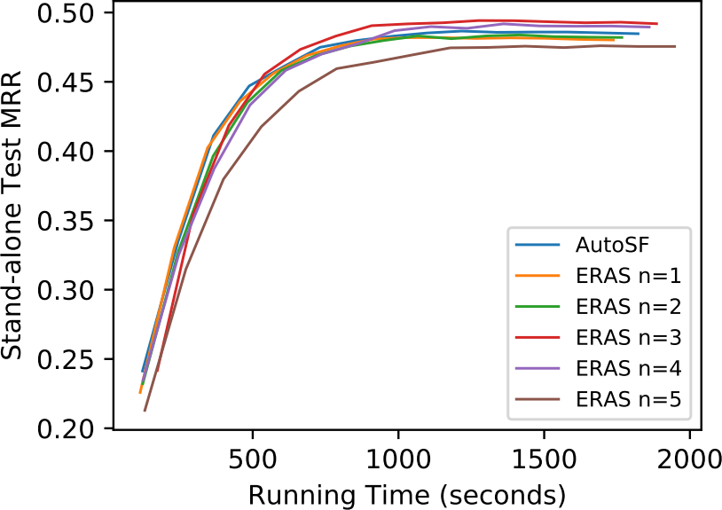
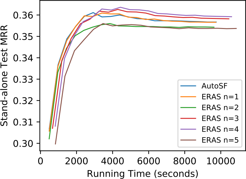
ERAS enables embedding sharing to improve the scoring function search efficiency. Hence we also compare the scoring function search efficiency of ERAS and with other automated search algorithms, i.e. AutoSF [14], random search [44], and Bayes algorithm [33], over three benchmark datasets. As shown in the Figure 2, both ERAS and complete the search very quickly. That is because other AutoML methods have to train hundreds of candidate scoring functions to convergence, while ERAS and avoids the time-consuming training by one-shot way. Compared with ERAS, convergess faster in search procedure since it does not dynamically assign relations and search corresponding scoring functions for different groups. It is worth noting that ERAS has unstable performance at beginning of the search. That is because FB15k237 has much more relations than another 2 data sets. It takes some time to find proper relation assignments at the start. Furthermore, other automated methods can achieve higher performance than ERAS in the search strategy. ERAS consistently updates the candidate scoring functions in every mini-batch data, which results in that the searched scoring functions cannot be well trained with one or several mini-batches. But other automated methods train the searched scoring functions with all training data until convergence.
We also summarize the running time on the five data sets in Table IX. AutoSF sets the embedding dimension to 64 for all data sets, while ERAS enables much faster search and hence sets . The larger dimensionality enables us to evaluate the scoring function more accurately. As shown in Table IX, the search time of AutoSF is significantly reduced by . But recall that the effectiveness of is the same with AutoSF in Table VI. This indicates that can extremely shorten the task-aware search time but maintain the same effectiveness with AutoSF. Moreover, although ERAS searches from a larger search space that is relation-aware, it reduces the search time of AutoSF by one order with a large dimension size and improves effectiveness as in Table VI. In summary, ERAS can more efficiently search for more effective scoring functions.
V-D Case Study: The Searched scoring functions
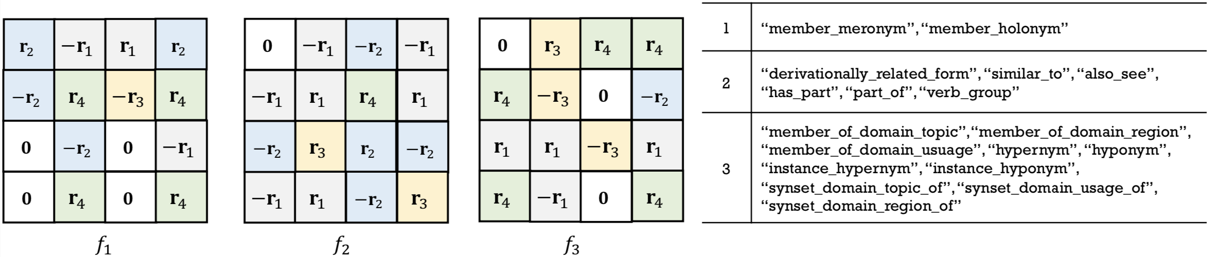
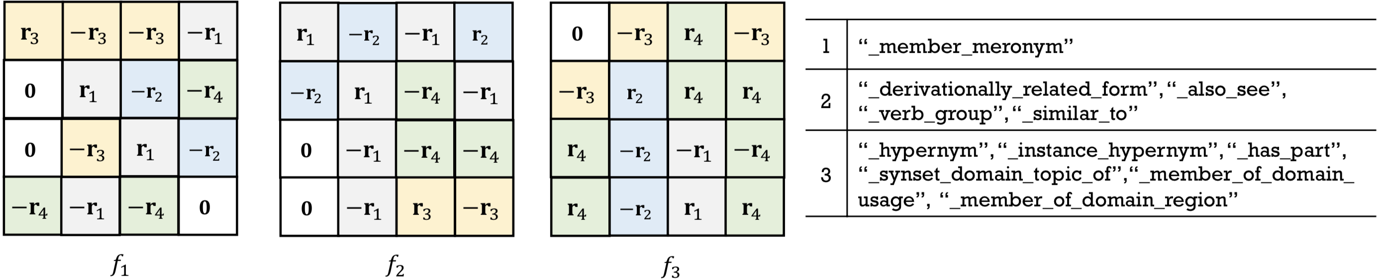
To show the searched scoring functions by ERAS are relation-aware, we use searched scoring functions from WN18 and WN18RR as examples and plot them in Figure 3 and 4. As we can see, the three searched scoring functions have distinct patterns and are relation-aware. Moreover, the relations are grouped into general asymmetry, symmetry, and anti-symmetry. And the three SFs searched have distinct patterns and can handle their corresponding relations.
V-E Ablation Study
To investigate the influence of different components of ERAS, we conduct several ablation studies.
V-E1 Impact of Evaluation Measurement and Optimization Algorithm
As discussed in Section IV-D2, the deep and complex supernet design will probably lead to the biased evaluation problem. In Figure 5(a), we first demonstrate the correlation between stand-alone validation MRR with one-shot validation MRR (i.e., ) of various scoring functions in ERAS. It is obvious that one-shot validation MRR has near positive correlation with the stand-alone validation MRR. Therefore, the simplified design of supernet makes embedding sharing work, and there is no biased evaluation problem.
To further investigate the impact of and optimization algorithms, we compare ERAS with following variants:
-
•
utilizes the validation loss to replace . Other steps are same with ERAS.
- •
We show the correlation between stand-alone validation MRR with different settings in Figure 5. Obviously, compared with using MRR as in Figure 5 (a), Figure 5 (b) shows that using as has a low correlation with stand-alone validation MRR. This indicates that validation loss in search strategy cannot well evaluate the stand-alone performance of scoring functions. Subsequently, in Table XI, we can observe that the performance of ERAS using MRR as is better than that of two variants, i.e., and . Moreover, is worse than because optimizing loss with the RL approach could not make use of the differentiable nature of .


| Section | Variant | WN18 | WN18RR | FB15K | FB15k237 | YAGO3-10 |
|---|---|---|---|---|---|---|
| MRR | MRR | MRR | MRR | MRR | ||
| V-E1 | 0.944 | 0.485 | 0.840 | 0.344 | 0.560 | |
| 0.949 | 0.485 | 0.848 | 0.355 | 0.565 | ||
| V-E2 | 0.945 | 0.480 | 0.844 | 0.338 | 0.559 | |
| V-E3 | 0.950 | 0.489 | 0.850 | 0.349 | 0.570 | |
| 0.948 | 0.485 | 0.845 | 0.347 | 0.565 | ||
| ERAS | 0.953 | 0.492 | 0.855 | 0.365 | 0.577 |
V-E2 Impact of Optimization Level
In this paper, Definition 2 formulates the problem with a bi-level optimization objective. As stated in Section III-B, bi-level optimization can benefit ERAS by updating the scoring functions and embeddings separately. To investigate the impact of optimization level, we add another variant of ERAS as , which utilizes the training set to update (3) in Definition 2 (i.e., single-level problem). In Table XI, compared with , ERAS demonstrates the bi-level optimization is needed because optimizing scoring functions on the validation set encourages ERAS to select scoring functions that generalize well rather than scoring functions that overfit on the training data.
V-E3 Impact of Grouping Approaches
To explore more about the influence of different grouping approaches, we set two variants of ERAS as follows:
-
•
does not update during search. Instead, it fixes groupings based on the embedding trained from SimplE.
-
•
groups relations based on their semantic meanings (i.e., symmetric, anti-symmetric, asymmetric and inverse).
We compare these two variants with ERAS as shown in Table XI. Generally, the performance of is unsatisfactory due to the bias between human understanding of relation groups with the proper groups derived from data. In short, the performance comparison also indicates the importance of dynamically assigning relation groups in the search strategy, which encourages relations to be assigned to the appropriate scoring function.
V-E4 Impact of Grouping Numbers
To investigate the impact of grouping numbers in ERAS, we summarize the performance of searched scoring functions by AutoSF and different settings of ERAS in Figure 6, i.e., () on WN18RR and FB15k237. Generally, the more groups there are, the longer the running time is. And ERAS achieves the best performance when or . Comparing AutoSF and , they have a similar learning curve since their model complexities are the same.
V-E5 Impact of Block Numbers
AutoSF fixes the block number to 4 due to the efficiency issue. Once is changed (e.g., or ), all design details in AutoSF must be re-done. On the contrary, the efficiency of ERAS allows more flexible settings of . Here we try in order to learn more about how the block number influences the ERAS performance. As shown in Figure 7, we can observe that does have excellent performance among .


VI Conclusion
In this paper, we propose a new automated machine learning (AutoML) method for designing scoring functions (scoring functions) in knowledge graph embedding. First, we design a relation-aware search space, which is motivated by our analysis of how existing scoring functions adapt to different relations. Then, we represent the new search space as a supernet in the form of a graph and propose to search through the supernet by one-shot architecture search methods. Experimental results on benchmark data sets well demonstrate not only the efficiency of our approach but also the competitive effectiveness.
VII Acknowledgements
This work is partially supported by National Key Research and Development Program of China Grant no. 2018AAA0101100, the Hong Kong RGC GRF Project 16202218 , CRF Project C6030-18G, C1031-18G, C5026-18G, AOE Project AoE/E-603/18, China NSFC No. 61729201, Guangdong Basic and Applied Basic Research Foundation 2019B151530001, Hong Kong ITC ITF grants ITS/044/18FX and ITS/470/18FX, Microsoft Research Asia Collaborative Research Grant, Didi-HKUST joint research lab project, and Wechat and Webank Research Grants.
References
- [1] M. Nickel, K. Murphy, V. Tresp, and E. Gabrilovich, “A review of relational machine learning for knowledge graphs,” Proceedings of the IEEE, vol. 104, no. 1, pp. 11–33, 2015.
- [2] Q. Wang, Z. Mao, B. Wang, and L. Guo, “Knowledge graph embedding: A survey of approaches and applications,” TKDE, vol. 29, no. 12, pp. 2724–2743, 2017.
- [3] D. Lukovnikov, A. Fischer, J. Lehmann, and S. Auer, “Neural network-based question answering over knowledge graphs on word and character level,” in WWW, pp. 1211–1220, 2017.
- [4] F. Zhang, N. J. Yuan, D. Lian, X. Xie, and W.-Y. Ma, “Collaborative knowledge base embedding for recommender systems,” in SIGKDD, pp. 353–362, 2016.
- [5] X. Wang, Y. Ye, and A. Gupta, “Zero-shot recognition via semantic embeddings and knowledge graphs,” in ICPR, pp. 6857–6866, 2018.
- [6] Y. Lin, X. Han, R. Xie, Z. Liu, and M. Sun, “Knowledge representation learning: A quantitative review,” tech. rep., 2018.
- [7] A. Bordes, N. Usunier, A. Garcia-Duran, J. Weston, and O. Yakhnenko, “Translating embeddings for modeling multi-relational data,” in NIPS, pp. 2787–2795, 2013.
- [8] Z. Wang, J. Zhang, J. Feng, and Z. Chen, “Knowledge graph embedding by translating on hyperplanes,” in AAAI, 2014.
- [9] Y. Lin, Z. Liu, M. Sun, Y. Liu, and X. Zhu, “Learning entity and relation embeddings for knowledge graph completion,” in AAAI, 2015.
- [10] Y. Wang, R. Gemulla, and H. Li, “On multi-relational link prediction with bilinear models,” in AAAI, 2018.
- [11] R. Socher, D. Chen, C. Manning, and A. Ng, “Reasoning with neural tensor networks for knowledge base completion,” in NIPS, 2013.
- [12] T. Dettmers, P. Minervini, P. Stenetorp, and S. Riedel, “Convolutional 2D knowledge graph embeddings,” in AAAI, 2018.
- [13] X. Dong, E. Gabrilovich, G. Heitz, W. Horn, N. Lao, K. Murphy, T. Strohmann, S. Sun, and W. Zhang, “Knowledge vault: A web-scale approach to probabilistic knowledge fusion,” in SIGKDD, 2014.
- [14] Y. Zhang, Q. Yao, W. Dai, and L. Chen, “AutoSF: Searching scoring functions for knowledge graph embedding,” in ICDE, pp. 433–444, 2020.
- [15] B. Yang, W. Yih, X. He, J. Gao, and L. Deng, “Embedding entities and relations for learning and inference in knowledge bases,” in ICLR, 2015.
- [16] T. Trouillon, C. R., É. Gaussier, J. Welbl, S. Riedel, and G. Bouchard, “Knowledge graph completion via complex tensor factorization,” JMLR, vol. 18, no. 1, pp. 4735–4772, 2017.
- [17] S. Kazemi and D. Poole, “Simple embedding for link prediction in knowledge graphs,” in NeurIPS, pp. 4284–4295, 2018.
- [18] H. Liu, Y. Wu, and Y. Yang, “Analogical inference for multi-relational embeddings,” in ICML, pp. 2168–2178, JMLR. org, 2017.
- [19] T. Lacroix, N. Usunier, and G. Obozinski, “Canonical tensor decomposition for knowledge base completion,” in ICML, pp. 2863–2872, 2018.
- [20] I. Balazevic, C. Allen, and T. Hospedales, “Tucker: Tensor factorization for knowledge graph completion,” in EMNLP-IJCNLP, pp. 5188–5197, 2019.
- [21] F. Hutter, L. Kotthoff, and J. Vanschoren, Automated Machine Learning: Methods, Systems, Challenges. Springer, 2018.
- [22] Q. Yao and M. Wang, “Taking human out of learning applications: A survey on automated machine learning,” tech. rep., arXiv:1810.13306, 2018.
- [23] M. Feurer, A. Klein, K. Eggensperger, J. Springenberg, M. Blum, and F. Hutter, “Efficient and robust automated machine learning,” in NIPS, pp. 2962–2970, 2015.
- [24] B. Zoph and Q. Le, “Neural architecture search with reinforcement learning,” in ICLR, 2016.
- [25] I. Balažević, C. Allen, and T. Hospedales, “Hypernetwork knowledge graph embeddings,” in ICANN, pp. 553–565, Springer, 2019.
- [26] M. Nickel, L. Rosasco, and T. Poggio, “Holographic embeddings of knowledge graphs,” in AAAI, 2016.
- [27] A. Rossi, D. Firmani, A. Matinata, P. Merialdo, and D. Barbosa, “Knowledge graph embedding for link prediction: A comparative analysis,” tech. rep., 2020.
- [28] C. Meilicke, M. Fink, Y. Wang, D. Ruffinelli, R. Gemulla, and H. Stuckenschmidt, “Fine-grained evaluation of rule-and embedding-based systems for knowledge graph completion,” in ISWC, pp. 3–20, 2018.
- [29] Y. Xue, Y. Yuan, Z. Xu, and A. Sabharwal, “Expanding holographic embeddings for knowledge completion,” in NeurIPS, pp. 4491–4501, 2018.
- [30] B. Colson, P. Marcotte, and G. Savard, “An overview of bilevel optimization,” Annals of Operations Research, vol. 153, no. 1, pp. 235–256, 2007.
- [31] Y. LeCun, “Gradient-based learning applied to document recognition,” in Proceedings of the IEEE, 1998.
- [32] G. E. H. Rumelhart, David E. and R. J. Williams, “Learning representations by back-propagating errors,” in Nature, 1986.
- [33] J. Bergstra, D. Yamins, and D. D. Cox, “Making a science of model search: Hyperparameter optimization in hundreds of dimensions for vision architectures,” 2013.
- [34] L. Xie and A. Yuille, “Genetic CNN,” in ICCV, pp. 1388–1397, 2017.
- [35] H. Pham, M. Guan, B. Zoph, Q. Le, and J. Dean, “Efficient neural architecture search via parameter sharing,” in ICML, pp. 4092–4101, 2018.
- [36] H. Liu, K. Simonyan, and Y. Yang, “DARTS: Differentiable architecture search,” in ICLR, 2018.
- [37] Q. Yao, J. Xu, W.-W. Tu, and Z. Zhu, “Efficient neural architecture search via proximal iterations,” in AAAI, 2020.
- [38] G. Bender, P.-J. Kinderm, B. Zoph, V. Vasudevan, and Q. Le, “Understanding and simplifying one-shot architecture search,” in ICML, pp. 549–558, 2018.
- [39] R. J. Williams, “Simple statistical gradient-following algorithms for connectionist reinforcement learning,” ML, vol. 8, no. 3-4, pp. 229–256, 1992.
- [40] M. Nickel, V. Tresp, and H. Kriegel, “A three-way model for collective learning on multi-relational data.,” in ICML, vol. 11, pp. 809–816, 2011.
- [41] K. Toutanova and D. Chen, “Observed versus latent features for knowledge base and text inference,” in Workshop on CVSMC, pp. 57–66, 2015.
- [42] A. Dempster, N. M. Laird, and D. Rubin, “Maximum likelihood from incomplete data via the em algorithm,” Journal of the Royal Statistical Society: Series B (Methodological), vol. 39, no. 1, pp. 1–22, 1977.
- [43] S. Hochreiter and J. Schmidhuber, “Long short-term memory,” Neural Computation, vol. 9, no. 8, pp. 1735–1780, 1997.
- [44] L. Li and A. Talwalkar, “Random search and reproducibility for neural architecture search,” tech. rep., 2019.
- [45] Z. Sun, Z. Deng, J. Nie, and J. Tang, “RotatE: Knowledge graph embedding by relational rotation in complex space,” in ICLR, 2019.
- [46] S. Zhang, Y. Tay, L. Yao, and Q. Liu, “Quaternion knowledge graph embeddings,” in NeurIPS, pp. 2731–2741, 2019.
- [47] A. Paszke, S. Gross, F. Massa, A. Lerer, J. Bradbury, G. Chanan, T. Killeen, Z. Lin, N. Gimelshein, L. Antiga, et al., “Pytorch: An imperative style, high-performance deep learning library,” in NeurIPS, pp. 8024–8035, 2019.
- [48] J. Duchi, E. Hazan, and Y. Singer, “Adaptive subgradient methods for online learning and stochastic optimization,” JMLR, vol. 12, no. Jul, pp. 2121–2159, 2011.
- [49] D. Kingma and J. Ba, “Adam: A method for stochastic optimization,” in ICLR, 2014.
- [50] C. Meilicke, M. W. Chekol, D. Ruffinelli, and H. Stuckenschmidt, “Anytime bottom-up rule learning for knowledge graph completion,” in IJCAI, pp. 3137–3143, 2019.
- [51] J. Zhou, G. Cui, Z. Zhang, C. Yang, Z. Liu, L. Wang, C. Li, and M. Sun, “Graph neural networks: A review of methods and applications,” tech. rep., 2018.
- [52] Y. Zhang, Q. Yao, and L. Chen, “Interstellar: Searching recurrent architecture forknowledge graph embedding,” in NeurIPS, 2019.
Details of Implementing
We propose a supernet view of the scoring function search space as in (8). This supernet design allows us to employ differentiable OAS methods when we use the loss as . Following NASP [37], can update the architecture weight by gradient descent as:
Then (3) can be optimized by above equation. Other steps of are same with ERAS.