Efficient Second Order Online Learning by Sketching

Haipeng Luo
Princeton University, Princeton, NJ USA
haipengl@cs.princeton.edu
&Alekh Agarwal
Microsoft Research, New York, NY USA
alekha@microsoft.com
&Nicolò Cesa-Bianchi
Università degli Studi di Milano, Italy
nicolo.cesa-bianchi@unimi.it
&John Langford
Microsoft Research, New York, NY USA
jcl@microsoft.com

Abstract

We propose Sketched Online Newton (SON), an online second order learning algorithm that enjoys substantially improved regret guarantees for ill-conditioned data. SON is an enhanced version of the Online Newton Step, which, via sketching techniques enjoys a running time linear in the dimension and sketch size. We further develop sparse forms of the sketching methods (such as Oja’s rule), making the computation linear in the sparsity of features. Together, the algorithm eliminates all computational obstacles in previous second order online learning approaches.

1 Introduction

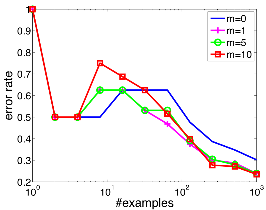
Online learning methods are highly successful at rapidly reducing the test error on large, high-dimensional datasets. First order methods are particularly attractive in such problems as they typically enjoy computational complexity linear in the input size. However, the convergence of these methods crucially depends on the geometry of the data; for instance, running the same algorithm on a rotated set of examples can return vastly inferior results. See Fig. 1 for an illustration.

Second order algorithms such as Online Newton Step (Hazan et al., 2007) have the attractive property of being invariant to linear transformations of the data, but typically require space and update time quadratic in the number of dimensions. Furthermore, the dependence on dimension is not improved even if the examples are sparse. These issues lead to the key question in our work: Can we develop (approximately) second order online learning algorithms with efficient updates? We show that the answer is “yes” by developing efficient sketched second order methods with regret guarantees. Specifically, the three main contributions of this work are:

Refer to caption — Figure 1: Error rate of SON using Oja’s sketch, and AdaGrad on a synthetic ill-conditioned problem. $m$ is the sketch size ( $m=0$ is Online Gradient, $m=d$ resembles Online Newton). SON is nearly invariant to condition number for $m=10$ .

1. Invariant learning setting and optimal algorithms (Section 2).

The typical online regret minimization setting evaluates against a benchmark that is bounded in some fixed norm (such as the $\ell_{2}$ -norm), implicitly putting the problem in a nice geometry. However, if all the features are scaled down, it is desirable to compare with accordingly larger weights, which is precluded by an apriori fixed norm bound. We study an invariant learning setting similar to the paper (Ross et al., 2013) which compares the learner to a benchmark only constrained to generate bounded predictions on the sequence of examples. We show that a variant of the Online Newton Step (Hazan et al., 2007), while quadratic in computation, stays regret-optimal with a nearly matching lower bound in this more general setting.

2. Improved efficiency via sketching (Section 3).

To overcome the quadratic running time, we next develop sketched variants of the Newton update, approximating the second order information using a small number of carefully chosen directions, called a sketch. While the idea of data sketching is widely studied (Woodruff, 2014), as far as we know our work is the first one to apply it to a general adversarial online learning setting and provide rigorous regret guarantees. Two different sketching methods are considered: Frequent Directions (Ghashami et al., 2015; Liberty, 2013) and Oja’s algorithm (Oja, 1982; Oja and Karhunen, 1985), both of which allow linear running time per round. For the first method, we prove regret bounds similar to the full second order update whenever the sketch-size is large enough. Our analysis makes it easy to plug in other sketching and online PCA methods (e.g. (Garber et al., 2015)).

3. Sparse updates (Section 4).

For practical implementation, we further develop sparse versions of these updates with a running time linear in the sparsity of the examples. The main challenge here is that even if examples are sparse, the sketch matrix still quickly becomes dense. These are the first known sparse implementations of the Frequent Directions¹¹1Recent work by (Ghashami et al., 2016) also studies sparse updates for a more complicated variant of Frequent Directions which is randomized and incurs extra approximation error. and Oja’s algorithm, and require new sparse eigen computation routines that may be of independent interest.

Empirically, we evaluate our algorithm using the sparse Oja sketch (called Oja-SON) against first order methods such as diagonalized AdaGrad (Duchi et al., 2011; McMahan and Streeter, 2010) on both ill-conditioned synthetic and a suite of real-world datasets. As Fig. 1 shows for a synthetic problem, we observe substantial performance gains as data conditioning worsens. On the real-world datasets, we find improvements in some instances, while observing no substantial second-order signal in the others.

Related work

Our online learning setting is closest to the one proposed in (Ross et al., 2013), which studies scale-invariant algorithms, a special case of the invariance property considered here (see also (Orabona et al., 2015, Section 5)). Computational efficiency, a main concern in this work, is not a problem there since each coordinate is scaled independently. Orabona and Pál (2015) study unrelated notions of invariance. Gao et al. (2013) study a specific randomized sketching method for a special online learning setting.

The L-BFGS algorithm (Liu and Nocedal, 1989) has recently been studied in the stochastic setting²²2Stochastic setting assumes that the examples are drawn i.i.d. from a distribution. (Byrd et al., 2016; Mokhtari and Ribeiro, 2015; Moritz et al., 2016; Schraudolph et al., 2007; Sohl-Dickstein et al., 2014), but has strong assumptions with pessimistic rates in theory and reliance on the use of large mini-batches empirically. Recent works (Erdogdu and Montanari, 2015; Gonen et al., 2016; Gonen and Shalev-Shwartz, 2015; Pilanci and Wainwright, 2015) employ sketching in stochastic optimization, but do not provide sparse implementations or extend in an obvious manner to the online setting. The Frank-Wolfe algorithm (Frank and Wolfe, 1956; Jaggi, 2013) is also invariant to linear transformations, but with worse regret bounds (Hazan and Kale, 2012) without further assumptions and modifications (Garber and Hazan, 2016).

Notation

Vectors are represented by bold letters (e.g., $\boldsymbol{x}$ , $\boldsymbol{w}$ , …) and matrices by capital letters (e.g., $M$ , $A$ , …). $M_{i,j}$ denotes the $(i,j)$ entry of matrix $M$ . $\boldsymbol{I}_{d}$ represents the $d\times d$ identity matrix, $\boldsymbol{0}_{m\times d}$ represents the $m\times d$ matrix of zeroes, and $\mathrm{diag}\!\left\{{\boldsymbol{x}}\right\}$ represents a diagonal matrix with $\boldsymbol{x}$ on the diagonal. $\lambda_{i}(A)$ denotes the $i$ -th largest eigenvalue of $A$ , $\left\|{\boldsymbol{w}}\right\|_{A}$ denotes $\sqrt{\boldsymbol{w}^{\top}A\boldsymbol{w}}$ , $|A|$ is the determinant of $A$ , $\textsc{tr}({A})$ is the trace of $A$ , $\left\langle{A,B}\right\rangle$ denotes $\sum_{i,j}A_{i,j}B_{i,j}$ , and $A\preceq B$ means that $B-A$ is positive semidefinite. The sign function $\mbox{\sc sgn}(a)$ is $1$ if $a\geq 0$ and $-1$ otherwise.

2 Setup and an Optimal Algorithm

We consider the following setting. On each round $t=1,2\ldots,T$ : (1) the adversary first presents an example $\boldsymbol{x}_{t}\in\mathbb{R}^{d}$ , (2) the learner chooses $\boldsymbol{w}_{t}\in\mathbb{R}^{d}$ and predicts $\boldsymbol{w}_{t}^{\top}\boldsymbol{x}_{t}$ , (3) the adversary reveals a loss function $f_{t}(\boldsymbol{w})=\ell_{t}(\boldsymbol{w}^{\top}\boldsymbol{x}_{t})$ for some convex, differentiable $\ell_{t}:\mathbb{R}\rightarrow\mathbb{R}_{+}$ , and (4) the learner suffers loss $f_{t}(\boldsymbol{w}_{t})$ for this round.

The learner’s regret to a comparator $\boldsymbol{w}$ is defined as $R_{T}(\boldsymbol{w})=\sum_{t=1}^{T}f_{t}(\boldsymbol{w}_{t})-\sum_{t=1}^{T}f_{t}(\boldsymbol{w})$ . Typical results study $R_{T}(\boldsymbol{w})$ against all $\boldsymbol{w}$ with a bounded norm in some geometry. For an invariant update, we relax this requirement and only put bounds on the predictions $\boldsymbol{w}^{\top}\boldsymbol{x}_{t}$ . Specifically, for some pre-chosen constant $C$ we define $\mathcal{K}_{t}\stackrel{{\scriptstyle\rm def}}{{=}}\left\{{\boldsymbol{w}}\,:\,{|\boldsymbol{w}^{\top}\boldsymbol{x}_{t}|\leq C}\right\}.$ We seek to minimize regret to all comparators that generate bounded predictions on every data point, that is:

R_{T}=\sup_{\boldsymbol{w}\in\mathcal{K}}R_{T}(\boldsymbol{w})~~\mbox{ where}~~\mathcal{K}\stackrel{{\scriptstyle\rm def}}{{=}}\bigcap_{t=1}^{T}\mathcal{K}_{t}=\left\{{\boldsymbol{w}}\,:\,{\forall t=1,2,\ldots T,~~|\boldsymbol{w}^{\top}\boldsymbol{x}_{t}|\leq C}\right\}~.

Under this setup, if the data are transformed to $M\boldsymbol{x}_{t}$ for all $t$ and some invertible matrix $M\in\mathbb{R}^{d\times d}$ , the optimal $\boldsymbol{w}^{*}$ simply moves to $(M^{-1})^{\top}\boldsymbol{w}^{*}$ , which still has bounded predictions but might have significantly larger norm. This relaxation is similar to the comparator set considered in (Ross et al., 2013).

We make two structural assumptions on the loss functions.

Assumption 1.

(Scalar Lipschitz) The loss function $\ell_{t}$ satisfies $|\ell_{t}^{{}^{\prime}}(z)|\leq L$ whenever $|z|\leq C$ .

Assumption 2.

(Curvature) There exists $\sigma_{t}\geq 0$ such that for all $\boldsymbol{u},\boldsymbol{w}\in\mathcal{K}$ , $f_{t}(\boldsymbol{w})$ is lower bounded by $f_{t}(\boldsymbol{u})+\nabla f_{t}(\boldsymbol{u})^{\top}(\boldsymbol{w}-\boldsymbol{u})+\frac{\sigma_{t}}{2}\left(\nabla f_{t}(\boldsymbol{u})^{\top}(\boldsymbol{u}-\boldsymbol{w})\right)^{2}.$

Note that when $\sigma_{t}=0$ , Assumption 2 merely imposes convexity. More generally, it is satisfied by squared loss $f_{t}(\boldsymbol{w})=(\boldsymbol{w}^{\top}\boldsymbol{x}_{t}-y_{t})^{2}$ with $\sigma_{t}=\frac{1}{8C^{2}}$ whenever $|\boldsymbol{w}^{\top}\boldsymbol{x}_{t}|$ and $|y_{t}|$ are bounded by $C$ , as well as for all exp-concave functions (see (Hazan et al., 2007, Lemma 3)).

Enlarging the comparator set might result in worse regret. We next show matching upper and lower bounds qualitatively similar to the standard setting, but with an extra unavoidable $\sqrt{d}$ factor. ³³3In the standard setting where $\boldsymbol{w}_{t}$ and $\boldsymbol{x}_{t}$ are restricted such that $\left\|{\boldsymbol{w}_{t}}\right\|\leq D$ and $\left\|{\boldsymbol{x}_{t}}\right\|\leq X$ , the minimax regret is $\mathcal{O}(DXL\sqrt{T})$ . This is clearly a special case of our setting with $C=DX$ .

Theorem 1.

For any online algorithm generating $\boldsymbol{w}_{t}\in\mathbb{R}^{d}$ and all $T\geq d$ , there exists a sequence of $T$ examples $\boldsymbol{x}_{t}\in\mathbb{R}^{d}$ and loss functions $\ell_{t}$ satisfying Assumptions 1 and 2 (with $\sigma_{t}=0$ ) such that the regret $R_{T}$ is at least $CL\sqrt{dT/2}$ .

We now give an algorithm that matches the lower bound up to logarithmic constants in the worst case but enjoys much smaller regret when $\sigma_{t}\neq 0$ . At round $t+1$ with some invertible matrix $A_{t}$ specified later and gradient $\boldsymbol{g}_{t}=\nabla f_{t}(\boldsymbol{w}_{t})$ , the algorithm performs the following update before making the prediction on the example $\boldsymbol{x}_{t+1}$ :

\boldsymbol{u}_{t+1}=\boldsymbol{w}_{t}-A_{t}^{-1}\boldsymbol{g}_{t},\quad\mbox{and}\quad\boldsymbol{w}_{t+1}=\operatorname*{argmin}_{\boldsymbol{w}\in\mathcal{K}_{t+1}}\left\|{\boldsymbol{w}-\boldsymbol{u}_{t+1}}\right\|_{A_{t}}.

(1)

The projection onto the set $\mathcal{K}_{t+1}$ differs from typical norm-based projections as it only enforces boundedness on $\boldsymbol{x}_{t+1}$ at round $t+1$ . Moreover, this projection step can be performed in closed form.

Lemma 1.

For any $\boldsymbol{x}\neq\boldsymbol{0},\boldsymbol{u}\in\mathbb{R}^{d}$ and positive definite matrix $A\in\mathbb{R}^{d\times d}$ , we have

\operatorname*{argmin}_{\boldsymbol{w}\,:\,|\boldsymbol{w}^{\top}\boldsymbol{x}|\leq C}\left\|{\boldsymbol{w}-\boldsymbol{u}}\right\|_{A}=\boldsymbol{u}-\frac{\tau_{C}(\boldsymbol{u}^{\top}\boldsymbol{x})}{\boldsymbol{x}^{\top}A^{-1}\boldsymbol{x}}A^{-1}\boldsymbol{x},~~\mbox{where $\tau_{C}(y)=\mbox{\sc sgn}(y)\max\{|y|-C,0\}$.}

If $A_{t}$ is a diagonal matrix, updates similar to those of Ross et al. (2013) are recovered. We study a choice of $A_{t}$ that is similar to the Online Newton Step (ONS) (Hazan et al., 2007) (though with different projections):

A_{t}=\alpha\boldsymbol{I}_{d}+\sum_{s=1}^{t}(\sigma_{s}+\eta_{s})\boldsymbol{g}_{s}\boldsymbol{g}_{s}^{\top}

(2)

for some parameters $\alpha>0$ and $\eta_{t}\geq 0$ . The regret guarantee of this algorithm is shown below:

Theorem 2.

Under Assumptions 1 and 2, suppose that $\sigma_{t}\geq\sigma\geq 0$ for all $t$ , and $\eta_{t}$ is non-increasing. Then using the matrices (2) in the updates (1) yields for all $\boldsymbol{w}\in\mathcal{K}$ ,

\displaystyle R_{T}(\boldsymbol{w})\leq\frac{\alpha}{2}\left\|{\boldsymbol{w}}\right\|_{2}^{2}+2(CL)^{2}\sum_{t=1}^{T}\eta_{t}+\frac{d}{2(\sigma+\eta_{T})}\ln\left(1+\frac{(\sigma+\eta_{T})\sum_{t=1}^{T}\left\|{\boldsymbol{g}_{t}}\right\|_{2}^{2}}{d\alpha}\right)~.

The dependence on $\left\|{\boldsymbol{w}}\right\|_{2}^{2}$ implies that the method is not completely invariant to transformations of the data. This is due to the part $\alpha\boldsymbol{I}_{d}$ in $A_{t}$ . However, this is not critical since $\alpha$ is fixed and small while the other part of the bound grows to eventually become the dominating term. Moreover, we can even set $\alpha=0$ and replace the inverse with the Moore-Penrose pseudoinverse to obtain a truly invariant algorithm, as discussed in Appendix D. We use $\alpha>0$ in the remainder for simplicity.

The implication of this regret bound is the following: in the worst case where $\sigma=0$ , we set $\eta_{t}=\sqrt{d/C^{2}L^{2}t}$ and the bound simplifies to

\displaystyle R_{T}(\boldsymbol{w})\leq\frac{\alpha}{2}\left\|{\boldsymbol{w}}\right\|_{2}^{2}+\frac{CL}{2}\sqrt{Td}\ln\left(1+\frac{\sum_{t=1}^{T}\left\|{\boldsymbol{g}_{t}}\right\|_{2}^{2}}{\alpha CL\sqrt{Td}}\right)+4CL\sqrt{Td}~,

essentially only losing a logarithmic factor compared to the lower bound in Theorem 1. On the other hand, if $\sigma_{t}\geq\sigma>0$ for all $t$ , then we set $\eta_{t}=0$ and the regret simplifies to

R_{T}(\boldsymbol{w})\leq\frac{\alpha}{2}\left\|{\boldsymbol{w}}\right\|_{2}^{2}+\frac{d}{2\sigma}\ln\left(1+\frac{\sigma\sum_{t=1}^{T}\left\|{\boldsymbol{g}_{t}}\right\|_{2}^{2}}{d\alpha}\right)~,

(3)

extending the $\mathcal{O}(d\ln T)$ results in (Hazan et al., 2007) to the weaker Assumption 2 and a larger comparator set $\mathcal{K}$ .

3 Efficiency via Sketching

Our algorithm so far requires $\Omega(d^{2})$ time and space just as ONS. In this section we show how to achieve regret guarantees nearly as good as the above bounds, while keeping computation within a constant factor of first order methods.

Let $G_{t}\in\mathbb{R}^{t\times d}$ be a matrix such that the $t$ -th row is $\widehat{\boldsymbol{g}}_{t}^{\top}$ where we define $\widehat{\boldsymbol{g}}_{t}=\sqrt{\sigma_{t}+\eta_{t}}\boldsymbol{g}_{t}$ to be the to-sketch vector. Our previous choice of $A_{t}$ (Eq. (2)) can be written as $\alpha\boldsymbol{I}_{d}+G_{t}^{\top}G_{t}$ . The idea of sketching is to maintain an approximation of $G_{t}$ , denoted by $S_{t}\in\mathbb{R}^{m\times d}$ where $m\ll d$ is a small constant called the sketch size. If $m$ is chosen so that $S_{t}^{\top}S_{t}$ approximates $G_{t}^{\top}G_{t}$ well, we can redefine $A_{t}$ as $\alpha\boldsymbol{I}_{d}+S_{t}^{\top}S_{t}$ for the algorithm.

Algorithm 1 Sketched Online Newton (SON)

1:Parameters

C

\alpha

and

m

2:Initialize

\boldsymbol{u}_{1}=\boldsymbol{0}_{d\times 1}

3:Initialize sketch

(S,H)\leftarrow\textbf{SketchInit}(\alpha,m)

4:for

t=1

T

5: Receive example

\boldsymbol{x}_{t}

6: Projection step: compute

\widehat{\boldsymbol{x}}=S\boldsymbol{x}_{t},\;\gamma=\frac{\tau_{C}(\boldsymbol{u}_{t}^{\top}\boldsymbol{x}_{t})}{\boldsymbol{x}_{t}^{\top}\boldsymbol{x}_{t}-{\widehat{\boldsymbol{x}}}^{\top}H\widehat{\boldsymbol{x}}}

and set

\boldsymbol{w}_{t}=\boldsymbol{u}_{t}-\gamma(\boldsymbol{x}_{t}-S^{\top}H\widehat{\boldsymbol{x}})

7: Predict label

y_{t}=\boldsymbol{w}_{t}^{\top}\boldsymbol{x}_{t}

and suffer loss

\ell_{t}(y_{t})

8: Compute gradient

\boldsymbol{g}_{t}=\ell^{\prime}_{t}(y_{t})\boldsymbol{x}_{t}

and the to-sketch vector

\widehat{\boldsymbol{g}}=\sqrt{\sigma_{t}+\eta_{t}}\boldsymbol{g}_{t}

(S,H)\leftarrow

SketchUpdate(

\widehat{\boldsymbol{g}}

10: Update weight:

\boldsymbol{u}_{t+1}=\boldsymbol{w}_{t}-\frac{1}{\alpha}(\boldsymbol{g}_{t}-S^{\top}HS\boldsymbol{g}_{t})

11:end for

To see why this admits an efficient algorithm, notice that by the Woodbury formula one has $A_{t}^{-1}=\frac{1}{\alpha}\bigl{(}\boldsymbol{I}_{d}-S_{t}^{\top}(\alpha\boldsymbol{I}_{m}+S_{t}S_{t}^{\top})^{-1}S_{t}\bigr{)}.$ With the notation $H_{t}=(\alpha\boldsymbol{I}_{m}+S_{t}S_{t}^{\top})^{-1}\in\mathbb{R}^{m\times m}$ and $\gamma_{t}=\tau_{C}(\boldsymbol{u}_{t+1}^{\top}\boldsymbol{x}_{t+1})/(\boldsymbol{x}_{t+1}^{\top}\boldsymbol{x}_{t+1}-\boldsymbol{x}_{t+1}^{\top}S_{t}^{\top}H_{t}S_{t}\boldsymbol{x}_{t+1})$ , update (1) becomes:

\displaystyle\boldsymbol{u}_{t+1}=\boldsymbol{w}_{t}-\tfrac{1}{\alpha}\bigl{(}\boldsymbol{g}_{t}-S_{t}^{\top}H_{t}S_{t}\boldsymbol{g}_{t}\bigr{)},\quad\mbox{and}\quad\boldsymbol{w}_{t+1}

\displaystyle=\boldsymbol{u}_{t+1}-\gamma_{t}\bigl{(}\boldsymbol{x}_{t+1}-S_{t}^{\top}H_{t}S_{t}\boldsymbol{x}_{t+1}\bigr{)}~.

The operations involving $S_{t}\boldsymbol{g}_{t}$ or $S_{t}\boldsymbol{x}_{t+1}$ require only $\mathcal{O}(md)$ time, while matrix vector products with $H_{t}$ require only $\mathcal{O}(m^{2})$ . Altogether, these updates are at most $m$ times more expensive than first order algorithms as long as $S_{t}$ and $H_{t}$ can be maintained efficiently. We call this algorithm Sketched Online Newton (SON) and summarize it in Algorithm 1.

We now discuss two sketching techniques to maintain the matrices $S_{t}$ and $H_{t}$ efficiently, each requiring $\mathcal{O}(md)$ storage and time linear in $d$ .

Frequent Directions (FD).

Algorithm 2 FD-Sketch for FD-SON 1:

S

and

H

. 2: 3:Set

S=\boldsymbol{0}_{m\times d}

and

H=\tfrac{1}{\alpha}\boldsymbol{I}_{m}

. 4:Return

(S,H)

. 1: 2:Insert

\widehat{\boldsymbol{g}}

into the last row of

S

. 3:Compute eigendecomposition:

V^{\top}\Sigma V=S^{\top}S

and set

S=(\Sigma-\Sigma_{m,m}\boldsymbol{I}_{m})^{\frac{1}{2}}V

. 4:Set

H=\mathrm{diag}\!\left\{{\frac{1}{\alpha+\Sigma_{1,1}-\Sigma_{m,m}},\cdots,\frac{1}{\alpha}}\right\}

. 5:Return

(S,H)

Algorithm 3 Oja’s Sketch for Oja-SON 1:

t

\Lambda

V

and

H

. 2: 3:Set

t=0,\Lambda=\boldsymbol{0}_{m\times m},H=\tfrac{1}{\alpha}\boldsymbol{I}_{m}

and

V

to any

m\times d

matrix with orthonormal rows. 4:Return (

\boldsymbol{0}_{m\times d}

H

). 1: 2:Update

t\leftarrow t+1

\Lambda

and

V

as Eqn. 4. 3:Set

S=(t\Lambda)^{\frac{1}{2}}V

. 4:Set

H=\mathrm{diag}\!\left\{{\frac{1}{\alpha+t\Lambda_{1,1}},\cdots,\frac{1}{\alpha+t\Lambda_{m,m}}}\right\}

. 5:Return

(S,H)

Frequent Directions sketch (Ghashami et al., 2015; Liberty, 2013) is a deterministic sketching method. It maintains the invariant that the last row of $S_{t}$ is always $\boldsymbol{0}$ . On each round, the vector $\widehat{\boldsymbol{g}}_{t}^{\top}$ is inserted into the last row of $S_{t-1}$ , then the covariance of the resulting matrix is eigendecomposed into $V_{t}^{\top}\Sigma_{t}V_{t}$ and $S_{t}$ is set to $(\Sigma_{t}-\rho_{t}\boldsymbol{I}_{m})^{\frac{1}{2}}V_{t}$ where $\rho_{t}$ is the smallest eigenvalue. Since the rows of $S_{t}$ are orthogonal to each other, $H_{t}$ is a diagonal matrix and can be maintained efficiently (see Algorithm 2). The sketch update works in $\mathcal{O}(md)$ time (see (Ghashami et al., 2015) and Appendix F) so the total running time is $\mathcal{O}(md)$ per round. We call this combination FD-SON and prove the following regret bound with notation $\Omega_{k}=\sum_{i=k+1}^{d}\lambda_{i}(G_{T}^{\top}G_{T})$ for any $k=0,\dots,m-1$ .

Theorem 3.

Under Assumptions 1 and 2, suppose that $\sigma_{t}\geq\sigma\geq 0$ for all $t$ and $\eta_{t}$ is non-increasing. FD-SON ensures that for any $\boldsymbol{w}\in\mathcal{K}$ and $k=0,\ldots,m-1$ , we have

\displaystyle R_{T}(\boldsymbol{w})\leq\frac{\alpha}{2}\left\|{\boldsymbol{w}}\right\|_{2}^{2}+2(CL)^{2}\sum_{t=1}^{T}\eta_{t}+\frac{m}{2(\sigma+\eta_{T})}\ln\left(1+\frac{\textsc{tr}({S_{T}^{\top}S_{T}})}{m\alpha}\right)+\frac{m\Omega_{k}}{2(m-k)(\sigma+\eta_{T})\alpha}~.

The bound depends on the spectral decay $\Omega_{k}$ , which essentially is the only extra term compared to the bound in Theorem 2. Similarly to previous discussion, if $\sigma_{t}\geq\sigma$ , we get the bound $\frac{\alpha}{2}\left\|{w}\right\|_{2}^{2}+\frac{m}{2\sigma}\ln\left(1+\frac{\textsc{tr}({S_{T}^{\top}S_{T}})}{m\alpha}\right)+\frac{m\Omega_{k}}{2(m-k)\sigma\alpha}~.$ With $\alpha$ tuned well, we pay logarithmic regret for the top $m$ eigenvectors, but a square root regret $\mathcal{O}(\sqrt{\Omega_{k}})$ for remaining directions not controlled by our sketch. This is expected for deterministic sketching which focuses on the dominant part of the spectrum. When $\alpha$ is not tuned we still get sublinear regret as long as $\Omega_{k}$ is sublinear.

Oja’s Algorithm.

Oja’s algorithm (Oja, 1982; Oja and Karhunen, 1985) is not usually considered as a sketching algorithm but seems very natural here. This algorithm uses online gradient descent to find eigenvectors and eigenvalues of data in a streaming fashion, with the to-sketch vector $\widehat{\boldsymbol{g}}_{t}$ ’s as the input. Specifically, let $V_{t}\in\mathbb{R}^{m\times d}$ denote the estimated eigenvectors and the diagonal matrix $\Lambda_{t}\in\mathbb{R}^{m\times m}$ contain the estimated eigenvalues at the end of round $t$ . Oja’s algorithm updates as:

\displaystyle\Lambda_{t}=(\boldsymbol{I}_{m}-\Gamma_{t})\Lambda_{t-1}+\Gamma_{t}\;\mathrm{diag}\!\left\{{V_{t-1}\widehat{\boldsymbol{g}}_{t}}\right\}^{2},\quad\quad V_{t}\xleftarrow{\text{orth}}V_{t-1}+\Gamma_{t}V_{t-1}\widehat{\boldsymbol{g}}_{t}\widehat{\boldsymbol{g}}_{t}^{\top}

(4)

where $\Gamma_{t}\in\mathbb{R}^{m\times m}$ is a diagonal matrix with (possibly different) learning rates of order $\Theta(1/t)$ on the diagonal, and the “ $\xleftarrow{\text{orth}}$ ” operator represents an orthonormalizing step.⁴⁴4For simplicity, we assume that $V_{t-1}+\Gamma_{t}V_{t-1}\widehat{\boldsymbol{g}}_{t}\widehat{\boldsymbol{g}}_{t}^{\top}$ is always of full rank so that the orthonormalizing step does not reduce the dimension of $V_{t}$ . The sketch is then $S_{t}=(t\Lambda_{t})^{\frac{1}{2}}V_{t}$ . The rows of $S_{t}$ are orthogonal and thus $H_{t}$ is an efficiently maintainable diagonal matrix (see Algorithm 3). We call this combination Oja-SON.

The time complexity of Oja’s algorithm is $\mathcal{O}(m^{2}d)$ per round due to the orthonormalizing step. To improve the running time to $\mathcal{O}(md)$ , one can only update the sketch every $m$ rounds (similar to the block power method (Hardt and Price, 2014; Li et al., 2015)). The regret guarantee of this algorithm is unclear since existing analysis for Oja’s algorithm is only for the stochastic setting (see e.g. (Balsubramani et al., 2013; Li et al., 2015)). However, Oja-SON provides good performance experimentally.

4 Sparse Implementation

In many applications, examples (and hence gradients) are sparse in the sense that $\left\|{\boldsymbol{x}_{t}}\right\|_{0}\leq s$ for all $t$ and some small constant $s\ll d$ . Most online first order methods enjoy a per-example running time depending on $s$ instead of $d$ in such settings. Achieving the same for second order methods is more difficult since $A_{t}^{-1}\boldsymbol{g}_{t}$ (or sketched versions) are typically dense even if $\boldsymbol{g}_{t}$ is sparse.

We show how to implement our algorithms in sparsity-dependent time, specifically, in $\mathcal{O}(m^{2}+ms)$ for FD-SON and in $\mathcal{O}(m^{3}+ms)$ for Oja-SON. We emphasize that since the sketch would still quickly become a dense matrix even if the examples are sparse, achieving purely sparsity-dependent time is highly non-trivial and may be of independent interest. Due to space limit, below we only briefly mention how to do it for Oja-SON. Similar discussion for the FD sketch can be found in Appendix F. Note that mathematically these updates are equivalent to the non-sparse counterparts and regret guarantees are thus unchanged.

There are two ingredients to doing this for Oja-SON: (1) The eigenvectors $V_{t}$ are represented as $V_{t}=F_{t}Z_{t}$ , where $Z_{t}\in\mathbb{R}^{m\times d}$ is a sparsely updatable direction (Step 3 in Algorithm 5) and $F_{t}\in\mathbb{R}^{m\times m}$ is a matrix such that $F_{t}Z_{t}$ is orthonormal. (2) The weights $\boldsymbol{w}_{t}$ are split as $\bar{\boldsymbol{w}}_{t}+Z_{t-1}^{\top}\boldsymbol{b}_{t}$ , where $\boldsymbol{b}_{t}\in\mathbb{R}^{m}$ maintains the weights on the subspace captured by $V_{t-1}$ (same as $Z_{t-1}$ ), and $\bar{\boldsymbol{w}}_{t}$ captures the weights on the complementary subspace which are again updated sparsely.

We describe the sparse updates for $\bar{\boldsymbol{w}}_{t}$ and $\boldsymbol{b}_{t}$ below with the details for $F_{t}$ and $Z_{t}$ deferred to Appendix G. Since $S_{t}=(t\Lambda_{t})^{\frac{1}{2}}V_{t}=(t\Lambda_{t})^{\frac{1}{2}}F_{t}Z_{t}$ and $\boldsymbol{w}_{t}=\bar{\boldsymbol{w}}_{t}+Z_{t-1}^{\top}\boldsymbol{b}_{t}$ , we know $\boldsymbol{u}_{t+1}$ is

\displaystyle\boldsymbol{w}_{t}-\big{(}\boldsymbol{I}_{d}-S_{t}^{\top}H_{t}S_{t}\big{)}\tfrac{\boldsymbol{g}_{t}}{\alpha}=\underbrace{\bar{\boldsymbol{w}}_{t}-\tfrac{\boldsymbol{g}_{t}}{\alpha}-(Z_{t}-Z_{t-1})^{\top}\boldsymbol{b}_{t}}_{\stackrel{{\scriptstyle\rm def}}{{=}}\bar{\boldsymbol{u}}_{t+1}}+Z_{t}^{\top}(\underbrace{\boldsymbol{b}_{t}+\tfrac{1}{\alpha}F_{t}^{\top}(t\Lambda_{t}H_{t})F_{t}Z_{t}\boldsymbol{g}_{t}}_{\stackrel{{\scriptstyle\rm def}}{{=}}\boldsymbol{b}_{t+1}^{\prime}})~.

(5)

Since $Z_{t}-Z_{t-1}$ is sparse by construction and the matrix operations defining $\boldsymbol{b}_{t+1}^{\prime}$ scale with $m$ , overall the update can be done in $\mathcal{O}(m^{2}+ms)$ . Using the update for $\boldsymbol{w}_{t+1}$ in terms of $\boldsymbol{u}_{t+1}$ , $\boldsymbol{w}_{t+1}$ is equal to

\displaystyle\boldsymbol{u}_{t+1}-\gamma_{t}(\boldsymbol{I}_{d}-S_{t}^{\top}H_{t}S_{t})\boldsymbol{x}_{t+1}=\underbrace{\bar{\boldsymbol{u}}_{t+1}-\gamma_{t}\boldsymbol{x}_{t+1}}_{\stackrel{{\scriptstyle\rm def}}{{=}}\bar{\boldsymbol{w}}_{t+1}}+Z_{t}^{\top}(\underbrace{\boldsymbol{b}_{t+1}^{\prime}+\gamma_{t}F_{t}^{\top}(t\Lambda_{t}H_{t})F_{t}Z_{t}\boldsymbol{x}_{t+1}}_{\stackrel{{\scriptstyle\rm def}}{{=}}\boldsymbol{b}_{t+1}})~.

(6)

Again, it is clear that all the computations scale with $s$ and not $d$ , so both $\bar{\boldsymbol{w}}_{t+1}$ and $\boldsymbol{b}_{t+1}$ require only $O(m^{2}+ms)$ time to maintain. Furthermore, the prediction $\boldsymbol{w}_{t}^{\top}\boldsymbol{x}_{t}=\bar{\boldsymbol{w}}_{t}^{\top}\boldsymbol{x}_{t}+\boldsymbol{b}_{t}^{\top}Z_{t-1}\boldsymbol{x}_{t}$ can also be computed in $\mathcal{O}(ms)$ time. The $\mathcal{O}(m^{3})$ in the overall complexity comes from a Gram-Schmidt step in maintaining $F_{t}$ (details in Appendix G).

The pseudocode is presented in Algorithms 4 and 5 with some details deferred to Appendix G. This is the first sparse implementation of online eigenvector computation to the best of our knowledge.

Algorithm 4 Sparse Sketched Online Newton with Oja’s Algorithm

1:Parameters

C

\alpha

and

m

2:Initialize

\bar{\boldsymbol{u}}=\boldsymbol{0}_{d\times 1}

and

\boldsymbol{b}=\boldsymbol{0}_{m\times 1}

3:(

\Lambda,F,Z,H)\leftarrow\textbf{SketchInit}(\alpha,m)

(Algorithm 5).

4:for

t=1

T

5: Receive example

\boldsymbol{x}_{t}

6: Projection step: compute

\widehat{\boldsymbol{x}}=FZ\boldsymbol{x}_{t}

and

\gamma=\frac{\tau_{C}(\bar{\boldsymbol{u}}^{\top}\boldsymbol{x}_{t}+\boldsymbol{b}^{\top}Z\boldsymbol{x}_{t})}{\boldsymbol{x}_{t}^{\top}\boldsymbol{x}_{t}-(t-1){\widehat{\boldsymbol{x}}}^{\top}\Lambda H\widehat{\boldsymbol{x}}}

. Obtain

\bar{\boldsymbol{w}}=\bar{\boldsymbol{u}}-\gamma\boldsymbol{x}_{t}

and

\boldsymbol{b}\leftarrow\boldsymbol{b}+\gamma(t-1)F^{\top}\Lambda H\widehat{\boldsymbol{x}}

(Equation 6).

7: Predict label

y_{t}=\bar{\boldsymbol{w}}^{\top}\boldsymbol{x}_{t}+\boldsymbol{b}^{\top}Z\boldsymbol{x}_{t}

and suffer loss

\ell_{t}(y_{t})

8: Compute gradient

\boldsymbol{g}_{t}=\ell^{\prime}_{t}(y_{t})\boldsymbol{x}_{t}

and the to-sketch vector

\widehat{\boldsymbol{g}}=\sqrt{\sigma_{t}+\eta_{t}}\boldsymbol{g}_{t}

9: (

\Lambda

F

Z

H

\boldsymbol{\delta}

)

\leftarrow

SketchUpdate(

\widehat{\boldsymbol{g}}

) (Algorithm 5).

10: Update weight:

\bar{\boldsymbol{u}}=\bar{\boldsymbol{w}}-\tfrac{1}{\alpha}\boldsymbol{g}_{t}-(\boldsymbol{\delta}^{\top}\boldsymbol{b})\widehat{\boldsymbol{g}}

and

\boldsymbol{b}\leftarrow\boldsymbol{b}+\tfrac{1}{\alpha}tF^{\top}\Lambda HFZ\boldsymbol{g}_{t}

(Equation 5).

11:end for

Algorithm 5 Sparse Oja’s Sketch

t

\Lambda

F

Z

H

and

K

3:Set

t=0,\Lambda=\boldsymbol{0}_{m\times m},F=K=\alpha H=\boldsymbol{I}_{m}

and

Z

to any

m\times d

matrix with orthonormal rows.

4:Return (

\Lambda

F

Z

H

2:Update

t\leftarrow t+1

. Pick a diagonal stepsize matrix

\Gamma_{t}

to update

\Lambda\leftarrow(\boldsymbol{I}-\Gamma_{t})\Lambda+\Gamma_{t}\;\mathrm{diag}\!\left\{{FZ\widehat{\boldsymbol{g}}}\right\}^{2}

3:Set

\boldsymbol{\delta}=A^{-1}\Gamma_{t}FZ\widehat{\boldsymbol{g}}

and update

K\leftarrow K+\boldsymbol{\delta}\widehat{\boldsymbol{g}}^{\top}Z^{\top}+Z\widehat{\boldsymbol{g}}\boldsymbol{\delta}^{\top}+(\widehat{\boldsymbol{g}}^{\top}\widehat{\boldsymbol{g}})\boldsymbol{\delta}\boldsymbol{\delta}^{\top}

4:Update

Z\leftarrow Z+\boldsymbol{\delta}\widehat{\boldsymbol{g}}^{\top}

(L,Q)\leftarrow\text{Decompose}(F,K)

(Algorithm 11), so that

LQZ=FZ

and

QZ

is orthogonal. Set

F=Q

6:Set

H\leftarrow\mathrm{diag}\!\left\{{\frac{1}{\alpha+t\Lambda_{1,1}},\cdots,\frac{1}{\alpha+t\Lambda_{m,m}}}\right\}

7:Return (

\Lambda

F

Z

H

\boldsymbol{\delta}

5 Experiments

Preliminary experiments revealed that out of our two sketching options, Oja’s sketch generally has better performance (see Appendix H). For more thorough evaluation, we implemented the sparse version of Oja-SON in Vowpal Wabbit.⁵⁵5An open source machine learning toolkit available at http://hunch.net/ṽw We compare it with AdaGrad (Duchi et al., 2011; McMahan and Streeter, 2010) on both synthetic and real-world datasets. Each algorithm takes a stepsize parameter: $\tfrac{1}{\alpha}$ serves as a stepsize for Oja-SON and a scaling constant on the gradient matrix for AdaGrad. We try both methods with the parameter set to $2^{j}$ for $j=-3,-2,\ldots,6$ and report the best results. We keep the stepsize matrix in Oja-SON fixed as $\Gamma_{t}=\frac{1}{t}\boldsymbol{I}_{m}$ throughout. All methods make one online pass over data minimizing square loss.

5.1 Synthetic Datasets

To investigate Oja-SON’s performance in the setting it is really designed for, we generated a range of synthetic ill-conditioned datasets as follows. We picked a random Gaussian matrix $Z\sim\mathbb{R}^{T\times d}$ ( $T=10,\!000$ and $d=100$ ) and a random orthonormal basis $V\in\mathbb{R}^{d\times d}$ . We chose a specific spectrum $\boldsymbol{\lambda}\in\mathbb{R}^{d}$ where the first $d-10$ coordinates are 1 and the rest increase linearly to some fixed condition number parameter $\kappa$ . We let $X=Z\mathrm{diag}\!\left\{{\boldsymbol{\lambda}}\right\}^{\frac{1}{2}}V^{\top}$ be our example matrix, and created a binary classification problem with labels $y=\mbox{sign}(\boldsymbol{\theta}^{\top}\boldsymbol{x})$ , where $\boldsymbol{\theta}\in\mathbb{R}^{d}$ is a random vector. We generated 20 such datasets with the same $Z,V$ and labels $y$ but different values of $\kappa\in\{10,20,\ldots,200$ }. Note that if the algorithm is truly invariant, it would have the same behavior on these 20 datasets.

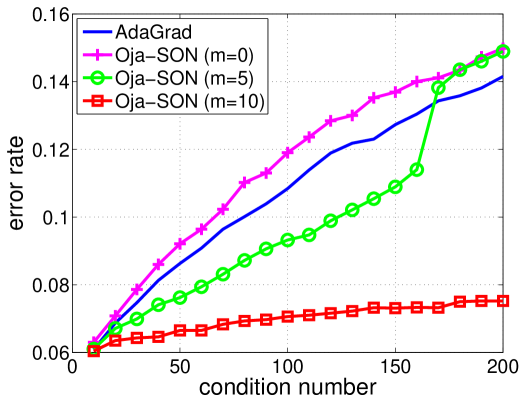
Fig. 1 (in Section 1) shows the final progressive error (i.e. fraction of misclassified examples after one pass over data) for AdaGrad and Oja-SON (with sketch size $m=0,5,10$ ) as the condition number increases. As expected, the plot confirms the performance of first order methods such as AdaGrad degrades when the data is ill-conditioned. The plot also shows that as the sketch size increases, Oja-SON becomes more accurate: when $m=0$ (no sketch at all), Oja-SON is vanilla gradient descent and is worse than AdaGrad as expected; when $m=5$ , the accuracy greatly improves; and finally when $m=10$ , the accuracy of Oja-SON is substantially better and hardly worsens with $\kappa$ .

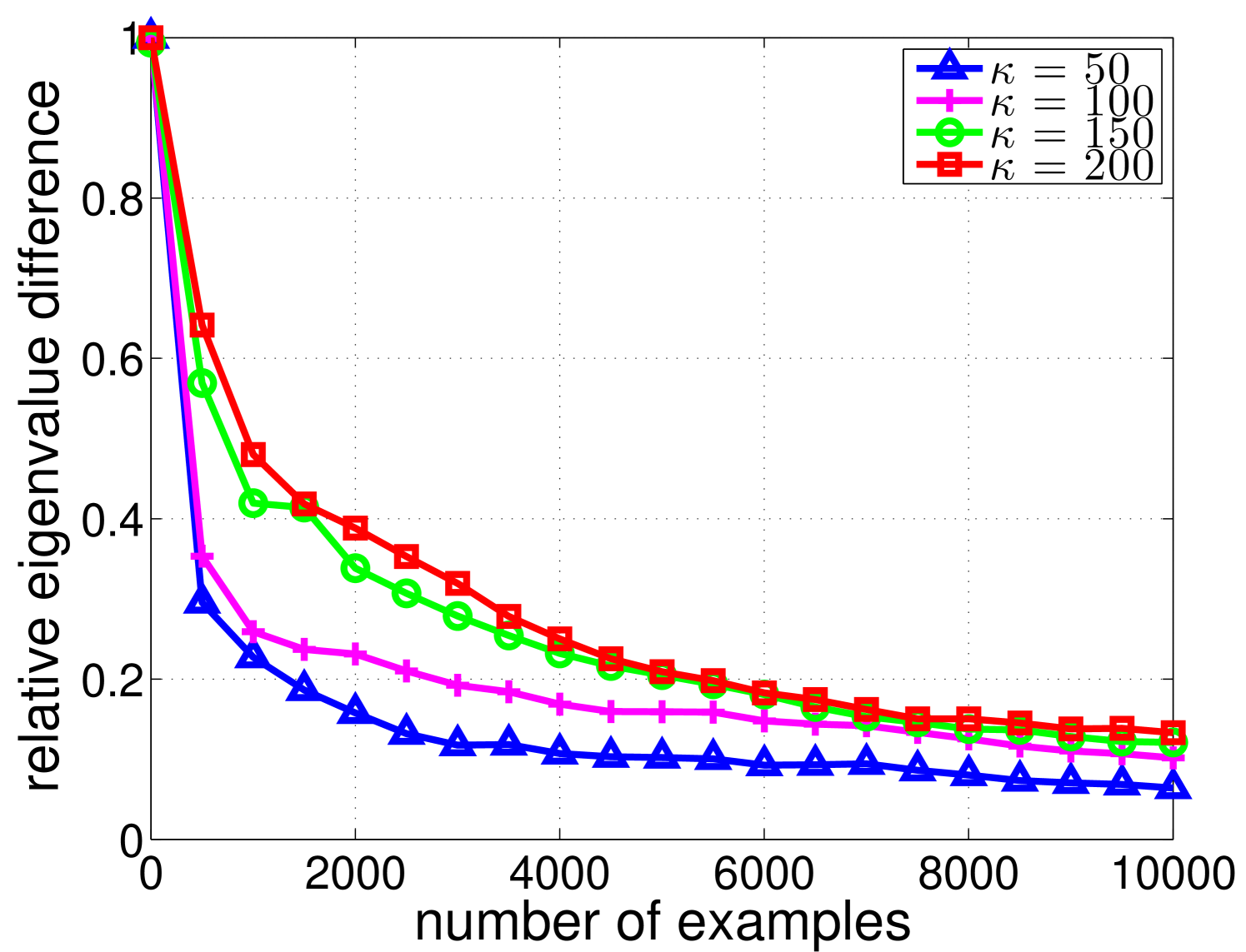
To further explain the effectiveness of Oja’s algorithm in identifying top eigenvalues and eigenvectors, the plot in Fig. 2 shows the largest relative difference between the true and estimated top 10 eigenvalues as Oja’s algorithm sees more data. This gap drops quickly after seeing just 500 examples.

5.2 Real-world Datasets

Next we evaluated Oja-SON on 23 benchmark datasets from the UCI and LIBSVM repository (see Appendix H for description of these datasets). Note that some datasets are very high dimensional but very sparse (e.g. for 20news, $d\approx 102,000$ and $s\approx 94$ ), and consequently methods with running time quadratic (such as ONS) or even linear in dimension rather than sparsity are prohibitive.

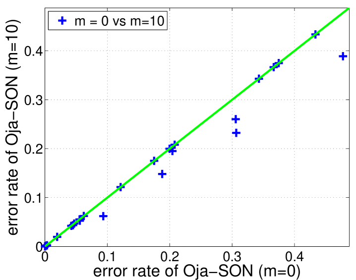
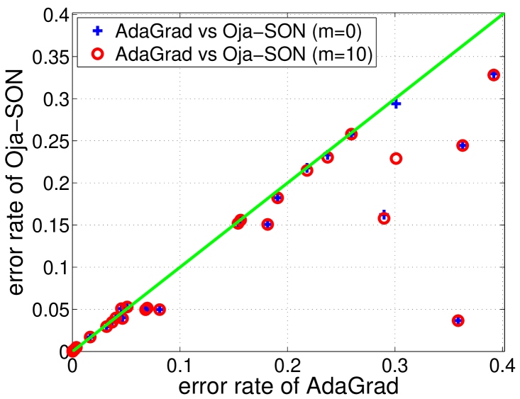
In Fig. 3, we show the effect of using sketched second order information, by comparing sketch size $m=0$ and $m=10$ for Oja-SON (concrete error rates in Appendix H). We observe significant improvements in 5 datasets (acoustic, census, heart, ionosphere, letter), demonstrating the advantage of using second order information. However, we found that Oja-SON was outperformed by AdaGrad on most datasets, mostly because the diagonal adaptation of AdaGrad greatly reduces the condition number on these datasets. Moreover, one disadvantage of SON is that for the directions not in the sketch, it is essentially doing vanilla gradient descent. We expect better results using diagonal adaptation as in AdaGrad in off-sketch directions.

To incorporate this high level idea, we performed a simple modification to Oja-SON: upon seeing example $\boldsymbol{x}_{t}$ , we feed $D_{t}^{-\frac{1}{2}}\boldsymbol{x}_{t}$ to our algorithm instead of $\boldsymbol{x}_{t}$ , where $D_{t}\in\mathbb{R}^{d\times d}$ is the diagonal part of the matrix $\sum_{\tau=1}^{t-1}\boldsymbol{g}_{\tau}\boldsymbol{g}_{\tau}^{\top}$ .⁶⁶6 $D_{1}$ is defined as $0.1\times\boldsymbol{I}_{d}$ to avoid division by zero. The intuition is that this diagonal rescaling first homogenizes the scales of all dimensions. Any remaining ill-conditioning is further addressed by the sketching to some degree, while the complementary subspace is no worse-off than with AdaGrad. We believe this flexibility in picking the right vectors to sketch is an attractive aspect of our sketching-based approach.

With this modification, Oja-SON outperforms AdaGrad on most of the datasets even for $m=0$ , as shown in Fig. 3 (concrete error rates in Appendix H). The improvement on AdaGrad at $m=0$ is surprising but not impossible as the updates are not identical–our update is scale invariant like Ross et al. (2013). However, the diagonal adaptation already greatly reduces the condition number on all datasets except splice (see Fig. 4 in Appendix H for detailed results on this dataset), so little improvement is seen for sketch size $m=10$ over $m=0$ . For several datasets, we verified the accuracy of Oja’s method in computing the top-few eigenvalues (Appendix H), so the lack of difference between sketch sizes is due to the lack of second order information after the diagonal correction.

The average running time of our algorithm when $m=10$ is about 11 times slower than AdaGrad, matching expectations. Overall, SON can significantly outperform baselines on ill-conditioned data, while maintaining a practical computational complexity.

Acknowledgements

This work was done when Haipeng Luo and Nicolò Cesa-Bianchi were at Microsoft Research, New York. We thank Lijun Zhang for pointing out our mistake in the regret proof of another sketching method that appeared in an earlier version.

References

Balsubramani et al. [2013] A. Balsubramani, S. Dasgupta, and Y. Freund. The fast convergence of incremental pca. In NIPS, 2013.
Byrd et al. [2016] R. H. Byrd, S. Hansen, J. Nocedal, and Y. Singer. A stochastic quasi-newton method for large-scale optimization. SIAM Journal on Optimization, 26:1008–1031, 2016.
Cesa-Bianchi and Lugosi [2006] N. Cesa-Bianchi and G. Lugosi. Prediction, Learning, and Games. Cambridge University Press, 2006.
Cesa-Bianchi et al. [2005] N. Cesa-Bianchi, A. Conconi, and C. Gentile. A second-order perceptron algorithm. SIAM Journal on Computing, 34(3):640–668, 2005.
Duchi et al. [2011] J. Duchi, E. Hazan, and Y. Singer. Adaptive subgradient methods for online learning and stochastic optimization. JMLR, 12:2121–2159, 2011.
Erdogdu and Montanari [2015] M. A. Erdogdu and A. Montanari. Convergence rates of sub-sampled newton methods. In NIPS, 2015.
Frank and Wolfe [1956] M. Frank and P. Wolfe. An algorithm for quadratic programming. Naval research logistics quarterly, 3(1-2):95–110, 1956.
Gao et al. [2013] W. Gao, R. Jin, S. Zhu, and Z.-H. Zhou. One-pass auc optimization. In ICML, 2013.
Garber and Hazan [2016] D. Garber and E. Hazan. A linearly convergent conditional gradient algorithm with applications to online and stochastic optimization. SIAM Journal on Optimization, 26:1493–1528, 2016.
Garber et al. [2015] D. Garber, E. Hazan, and T. Ma. Online learning of eigenvectors. In ICML, 2015.
Ghashami et al. [2015] M. Ghashami, E. Liberty, J. M. Phillips, and D. P. Woodruff. Frequent directions: Simple and deterministic matrix sketching. SIAM Journal on Computing, 45:1762–1792, 2015.
Ghashami et al. [2016] M. Ghashami, E. Liberty, and J. M. Phillips. Efficient frequent directions algorithm for sparse matrices. In KDD, 2016.
Gonen and Shalev-Shwartz [2015] A. Gonen and S. Shalev-Shwartz. Faster sgd using sketched conditioning. arXiv:1506.02649, 2015.
Gonen et al. [2016] A. Gonen, F. Orabona, and S. Shalev-Shwartz. Solving ridge regression using sketched preconditioned svrg. In ICML, 2016.
Hardt and Price [2014] M. Hardt and E. Price. The noisy power method: A meta algorithm with applications. In NIPS, 2014.
Hazan and Kale [2012] E. Hazan and S. Kale. Projection-free online learning. In ICML, 2012.
Hazan et al. [2007] E. Hazan, A. Agarwal, and S. Kale. Logarithmic regret algorithms for online convex optimization. Machine Learning, 69(2-3):169–192, 2007.
Jaggi [2013] M. Jaggi. Revisiting frank-wolfe: Projection-free sparse convex optimization. In ICML, 2013.
Li et al. [2015] C.-L. Li, H.-T. Lin, and C.-J. Lu. Rivalry of two families of algorithms for memory-restricted streaming pca. arXiv:1506.01490, 2015.
Liberty [2013] E. Liberty. Simple and deterministic matrix sketching. In KDD, 2013.
Liu and Nocedal [1989] D. C. Liu and J. Nocedal. On the limited memory bfgs method for large scale optimization. Mathematical programming, 45(1-3):503–528, 1989.
McMahan and Streeter [2010] H. B. McMahan and M. Streeter. Adaptive bound optimization for online convex optimization. In COLT, 2010.
Mokhtari and Ribeiro [2015] A. Mokhtari and A. Ribeiro. Global convergence of online limited memory bfgs. JMLR, 16:3151–3181, 2015.
Moritz et al. [2016] P. Moritz, R. Nishihara, and M. I. Jordan. A linearly-convergent stochastic l-bfgs algorithm. In AISTATS, 2016.
Oja [1982] E. Oja. Simplified neuron model as a principal component analyzer. Journal of mathematical biology, 15(3):267–273, 1982.
Oja and Karhunen [1985] E. Oja and J. Karhunen. On stochastic approximation of the eigenvectors and eigenvalues of the expectation of a random matrix. Journal of mathematical analysis and applications, 106(1):69–84, 1985.
Orabona and Pál [2015] F. Orabona and D. Pál. Scale-free algorithms for online linear optimization. In ALT, 2015.
Orabona et al. [2015] F. Orabona, K. Crammer, and N. Cesa-Bianchi. A generalized online mirror descent with applications to classification and regression. Machine Learning, 99(3):411–435, 2015.
Pilanci and Wainwright [2015] M. Pilanci and M. J. Wainwright. Newton sketch: A linear-time optimization algorithm with linear-quadratic convergence. arXiv:1505.02250, 2015.
Ross et al. [2013] S. Ross, P. Mineiro, and J. Langford. Normalized online learning. In UAI, 2013.
Schraudolph et al. [2007] N. N. Schraudolph, J. Yu, and S. Günter. A stochastic quasi-newton method for online convex optimization. In AISTATS, 2007.
Sohl-Dickstein et al. [2014] J. Sohl-Dickstein, B. Poole, and S. Ganguli. Fast large-scale optimization by unifying stochastic gradient and quasi-newton methods. In ICML, 2014.
Woodruff [2014] D. P. Woodruff. Sketching as a tool for numerical linear algebra. Foundations and Trends in Machine Learning, 10(1-2):1–157, 2014.

Supplementary material for
“Efficient Second Order Online Learning by Sketching”

Appendix A Proof of Theorem 1

Proof.

Assuming $T$ is a multiple of $d$ without loss of generality, we pick $\boldsymbol{x}_{t}$ from the basis vectors $\{\boldsymbol{e}_{1},\ldots,\boldsymbol{e}_{d}\}$ so that each $\boldsymbol{e}_{i}$ appears $T/d$ times (in an arbitrary order). Note that now $\mathcal{K}$ is just a hypercube:

\mathcal{K}=\left\{{\boldsymbol{w}}\,:\,{|\boldsymbol{w}^{\top}\boldsymbol{x}_{t}|\leq C,\;\;\forall t}\right\}=\left\{{\boldsymbol{w}}\,:\,{\left\|{\boldsymbol{w}}\right\|_{\infty}\leq C}\right\}.

Let $\xi_{1},\dots,\xi_{T}$ be independent Rademacher random variables such that $\Pr(\xi_{t}=+1)=\Pr(\xi_{t}=-1)=\tfrac{1}{2}$ . For a scalar $\theta$ , we define loss function⁷⁷7By adding a suitable constant, these losses can always be made nonnegative while leaving the regret unchanged. $\ell_{t}(\theta)=(\xi_{t}L)\theta$ , so that Assumptions 1 and 2 are clearly satisfied with $\sigma_{t}=0$ . We show that, for any online algorithm,

\mathbb{E}[R_{T}]=\mathbb{E}\left[\sum_{t=1}^{T}\ell_{t}\bigl{(}\boldsymbol{w}_{t}^{\top}\boldsymbol{x}_{t}\bigr{)}-\inf_{\boldsymbol{w}\in\mathcal{K}}\sum_{t=1}^{T}\ell_{t}\bigl{(}\boldsymbol{w}^{\top}\boldsymbol{x}_{t}\bigr{)}\right]\geq CL\sqrt{\frac{dT}{2}}

which implies the statement of the theorem.

First of all, note that $\mathbb{E}\Bigl{[}\ell_{t}\bigl{(}\boldsymbol{w}_{t}^{\top}\boldsymbol{x}_{t}\bigr{)}\,\Big{|}\,\xi_{1},\dots,\xi_{t-1}\Bigr{]}=0$ for any $\boldsymbol{w}_{t}$ . Hence we have

\displaystyle\mathbb{E}\left[\sum_{t=1}^{T}\ell_{t}\bigl{(}\boldsymbol{w}_{t}^{\top}\boldsymbol{x}_{t}\bigr{)}-\inf_{\boldsymbol{w}\in\mathcal{K}}\sum_{t=1}^{T}\ell_{t}\bigl{(}\boldsymbol{w}^{\top}\boldsymbol{x}_{t}\bigr{)}\right]

\displaystyle=\mathbb{E}\left[\sup_{\boldsymbol{w}\in\mathcal{K}}\sum_{t=1}^{T}-\ell_{t}\bigl{(}\boldsymbol{w}^{\top}\boldsymbol{x}_{t}\bigr{)}\right]=L\,\mathbb{E}\left[\sup_{\boldsymbol{w}\in\mathcal{K}}\boldsymbol{w}^{\top}\sum_{t=1}^{T}\xi_{t}\boldsymbol{x}_{t}\right],

which, by the construction of $\boldsymbol{x}_{t}$ , is

CL\,\mathbb{E}\left[\left\|{\sum_{t=1}^{T}\xi_{t}\boldsymbol{x}_{t}}\right\|_{1}\right]=CLd\,\mathbb{E}\left[\left|\sum_{t=1}^{T/d}\xi_{t}\right|\right]\geq CLd\sqrt{\frac{T}{2d}}=CL\sqrt{\frac{dT}{2}},

where the final bound is due to the Khintchine inequality (see e.g. Lemma 8.2 in Cesa-Bianchi and Lugosi [2006]). This concludes the proof. ∎

Appendix B Projection

We prove a more general version of Lemma 1 which does not require invertibility of the matrix $A$ here.

Lemma 2.

For any $\boldsymbol{x}\neq\boldsymbol{0},\boldsymbol{u}\in\mathbb{R}^{d\times 1}$ and positive semidefinite matrix $A\in\mathbb{R}^{d\times d}$ , we have

\boldsymbol{w}^{*}=\operatorname*{argmin}_{\boldsymbol{w}:|\boldsymbol{w}^{\top}\boldsymbol{x}|\leq C}\left\|{\boldsymbol{w}-\boldsymbol{u}}\right\|_{A}=\left\{\begin{array}[]{cl}\boldsymbol{u}-\frac{\tau_{C}(\boldsymbol{u}^{\top}\boldsymbol{x})}{\boldsymbol{x}^{\top}A^{\dagger}\boldsymbol{x}}A^{\dagger}\boldsymbol{x}&\text{if $\boldsymbol{x}\in\operatorname*{range}(A)$}\\ \\ \boldsymbol{u}-\frac{\tau_{C}(\boldsymbol{u}^{\top}\boldsymbol{x})}{\boldsymbol{x}^{\top}(\boldsymbol{I}-A^{\dagger}A)\boldsymbol{x}}(\boldsymbol{I}-A^{\dagger}A)\boldsymbol{x}&\text{if $\boldsymbol{x}\notin\operatorname*{range}(A)$}\end{array}\right.

where $\tau_{C}(y)=\mbox{\sc sgn}(y)\max\{|y|-C,0\}$ and $A^{\dagger}$ is the Moore-Penrose pseudoinverse of $A$ . (Note that when $A$ is rank deficient, this is one of the many possible solutions.)

Proof.

First consider the case when $\boldsymbol{x}\in\operatorname*{range}(A)$ . If $|\boldsymbol{u}^{\top}\boldsymbol{x}|\leq C$ , then it is trivial that $\boldsymbol{w}^{*}=\boldsymbol{u}$ . We thus assume $\boldsymbol{u}^{\top}\boldsymbol{x}\geq C$ below (the last case $\boldsymbol{u}^{\top}\boldsymbol{x}\leq-C$ is similar). The Lagrangian of the problem is

L(\boldsymbol{w},\lambda_{1},\lambda_{2})=\frac{1}{2}(\boldsymbol{w}-\boldsymbol{u})^{\top}A(\boldsymbol{w}-\boldsymbol{u})+\lambda_{1}(\boldsymbol{w}^{\top}\boldsymbol{x}-C)+\lambda_{2}(\boldsymbol{w}^{\top}\boldsymbol{x}+C)

where $\lambda_{1}\geq 0$ and $\lambda_{2}\leq 0$ are Lagrangian multipliers. Since $\boldsymbol{w}^{\top}\boldsymbol{x}$ cannot be $C$ and $-C$ at the same time, The complementary slackness condition implies that either $\lambda_{1}=0$ or $\lambda_{2}=0$ . Suppose the latter case is true, then setting the derivative with respect to $\boldsymbol{w}$ to $0$ , we get $\boldsymbol{w}^{*}=\boldsymbol{u}-\lambda_{1}A^{\dagger}\boldsymbol{x}+(\boldsymbol{I}-A^{\dagger}A)\boldsymbol{z}$ where $\boldsymbol{z}\in R^{d\times 1}$ can be arbitrary. However, since $A(\boldsymbol{I}-A^{\dagger}A)=0$ , this part does not affect the objective value at all and we can simply pick $z=0$ so that $w^{*}$ has a consistent form regardless of whether $A$ is full rank or not. Now plugging $\boldsymbol{w}^{*}$ back, we have

L(\boldsymbol{w}^{*},\lambda_{1},0)=-\frac{{\lambda_{1}}^{2}}{2}\boldsymbol{x}^{\top}A^{\dagger}\boldsymbol{x}+\lambda_{1}(\boldsymbol{u}^{\top}\boldsymbol{x}-C)

which is maximized when $\lambda_{1}=\frac{\boldsymbol{u}^{\top}\boldsymbol{x}-C}{\boldsymbol{x}^{\top}A^{\dagger}\boldsymbol{x}}\geq 0$ . Plugging this optimal $\lambda_{1}$ into $\boldsymbol{w}^{*}$ gives the stated solution. On the other hand, if $\lambda_{1}=0$ instead, we can proceed similarly and verify that it gives a smaller dual value ( $0$ in fact), proving the previous solution is indeed optimal.

We now move on to the case when $\boldsymbol{x}\notin\operatorname*{range}(A)$ . First of all the stated solution is well defined since $\boldsymbol{x}^{\top}(\boldsymbol{I}-A^{\dagger}A)\boldsymbol{x}$ is nonzero in this case. Moreover, direct calculation shows that $\boldsymbol{w}^{*}$ is in the valid space: $|{\boldsymbol{w}^{*}}^{\top}\boldsymbol{x}|=|\boldsymbol{u}^{\top}\boldsymbol{x}-\tau_{C}(\boldsymbol{u}^{\top}\boldsymbol{x})|\leq C$ , and also it gives the minimal possible distance value $\left\|{\boldsymbol{w}^{*}-\boldsymbol{u}}\right\|_{A}=0$ , proving the lemma. ∎

Appendix C Proof of Theorem 2

We first prove a general regret bound that holds for any choice of $A_{t}$ in update 1:

\begin{split}\boldsymbol{u}_{t+1}&=\boldsymbol{w}_{t}-A_{t}^{-1}\boldsymbol{g}_{t}\\ \boldsymbol{w}_{t+1}&=\operatorname*{argmin}_{\boldsymbol{w}\in\mathcal{K}_{t+1}}\left\|{\boldsymbol{w}-\boldsymbol{u}_{t+1}}\right\|_{A_{t}}~.\end{split}

This bound will also be useful in proving regret guarantees for the sketched versions.

Proposition 1.

For any sequence of positive definite matrices $A_{t}$ and sequence of losses satisfying Assumptions 1 and 2, the regret of updates (1) against any comparator $\boldsymbol{w}\in\mathcal{K}$ satisfies

2R_{T}(\boldsymbol{w})\leq\|\boldsymbol{w}\|_{A_{0}}^{2}+\underbrace{\sum_{t=1}^{T}\boldsymbol{g}_{t}^{T}A_{t}^{-1}\boldsymbol{g}_{t}}_{\text{``Gradient Bound'' $R_{G}$}}+\underbrace{\sum_{t=1}^{T}(\boldsymbol{w}_{t}-\boldsymbol{w})^{\top}(A_{t}-A_{t-1}-\sigma_{t}\boldsymbol{g}_{t}\boldsymbol{g}_{t}^{\top})(\boldsymbol{w}_{t}-\boldsymbol{w})}_{\text{``Diameter Bound'' $R_{D}$}}

Proof.

Since $\boldsymbol{w}_{t+1}$ is the projection of $\boldsymbol{u}_{t+1}$ onto $\mathcal{K}_{t+1}$ , by the property of projections (see for example [Hazan and Kale, 2012, Lemma 8]), the algorithm ensures

\left\|{\boldsymbol{w}_{t+1}-\boldsymbol{w}}\right\|_{A_{t}}^{2}\leq\left\|{\boldsymbol{u}_{t+1}-\boldsymbol{w}}\right\|_{A_{t}}^{2}=\left\|{\boldsymbol{w}_{t}-\boldsymbol{w}}\right\|_{A_{t}}^{2}+\boldsymbol{g}_{t}^{\top}A_{t}^{-1}\boldsymbol{g}_{t}-2\boldsymbol{g}_{t}^{\top}(\boldsymbol{w}_{t}-\boldsymbol{w})

for all $\boldsymbol{w}\in\mathcal{K}\subseteq\mathcal{K}_{t+1}$ . By the curvature property in Assumption 2, we then have that

	$\displaystyle 2R_{T}(\boldsymbol{w})\;$	$\displaystyle\leq\;\sum_{t=1}^{T}2\boldsymbol{g}_{t}^{\top}(\boldsymbol{w}_{t}-\boldsymbol{w})-\sigma_{t}\bigl{(}\boldsymbol{g}_{t}^{\top}(\boldsymbol{w}_{t}-\boldsymbol{w})\bigr{)}^{2}$
		$\displaystyle\leq\;\sum_{t=1}^{T}\boldsymbol{g}_{t}^{\top}A_{t}^{-1}\boldsymbol{g}_{t}+\left\\|{\boldsymbol{w}_{t}-\boldsymbol{w}}\right\\|_{A_{t}}^{2}-\left\\|{\boldsymbol{w}_{t+1}-\boldsymbol{w}}\right\\|_{A_{t}}^{2}-\sigma_{t}\bigl{(}\boldsymbol{g}_{t}^{\top}(\boldsymbol{w}_{t}-\boldsymbol{w})\bigr{)}^{2}$
		$\displaystyle\leq\;\left\\|{\boldsymbol{w}}\right\\|_{A_{0}}^{2}+\sum_{t=1}^{T}\boldsymbol{g}_{t}^{\top}A_{t}^{-1}\boldsymbol{g}_{t}+(\boldsymbol{w}_{t}-\boldsymbol{w})^{\top}(A_{t}-A_{t-1}-\sigma_{t}\boldsymbol{g}_{t}\boldsymbol{g}_{t}^{\top})(\boldsymbol{w}_{t}-\boldsymbol{w}),$

which completes the proof. ∎

Proof of Theorem 2.

We apply Proposition 1 with the choice: $A_{0}=\alpha\boldsymbol{I}_{d}$ and $A_{t}=A_{t-1}+(\sigma_{t}+\eta_{t})\boldsymbol{g}_{t}\boldsymbol{g}_{t}^{T}$ , which gives $\left\|{\boldsymbol{w}}\right\|_{A_{0}}^{2}=\alpha\left\|{\boldsymbol{w}}\right\|_{2}^{2}$ and

R_{D}=\sum_{t=1}^{T}\eta_{t}(\boldsymbol{w}_{t}-\boldsymbol{w})^{\top}\boldsymbol{g}_{t}\boldsymbol{g}_{t}^{\top}(\boldsymbol{w}_{t}-\boldsymbol{w})\leq 4(CL)^{2}\sum_{t=1}^{T}\eta_{t}~,

where the last equality uses the Lipschitz property in Assumption 1 and the boundedness of $\boldsymbol{w}_{t}^{\top}\boldsymbol{x}_{t}$ and $\boldsymbol{w}^{\top}\boldsymbol{x}_{t}$ .

For the term $R_{G}$ , define $\widehat{A}_{t}=\frac{\alpha}{\sigma+\eta_{T}}\boldsymbol{I}_{d}+\sum_{s=1}^{t}\boldsymbol{g}_{s}\boldsymbol{g}_{s}^{\top}$ . Since $\sigma_{t}\geq\sigma$ and $\eta_{t}$ is non-increasing, we have $\widehat{A}_{t}\preceq\frac{1}{\sigma+\eta_{T}}A_{t}$ , and therefore:

	$\displaystyle R_{G}$	$\displaystyle\leq\frac{1}{\sigma+\eta_{T}}\sum_{t=1}^{T}\boldsymbol{g}_{t}^{\top}\widehat{A}_{t}^{-1}\boldsymbol{g}_{t}=\frac{1}{\sigma+\eta_{T}}\sum_{t=1}^{T}\left\langle{\widehat{A}_{t}-\widehat{A}_{t-1},\;\widehat{A}_{t}^{-1}}\right\rangle$
		$\displaystyle\leq\frac{1}{\sigma+\eta_{T}}\sum_{t=1}^{T}\ln\frac{\|\widehat{A}_{t}\|}{\|\widehat{A}_{t-1}\|}=\frac{1}{\sigma+\eta_{T}}\ln\frac{\|\widehat{A}_{T}\|}{\|\widehat{A}_{0}\|}$
		$\displaystyle=\frac{1}{\sigma+\eta_{T}}\sum_{i=1}^{d}\ln\left(1+\frac{(\sigma+\eta_{T})\lambda_{i}\Bigl{(}\sum_{t=1}^{T}\boldsymbol{g}_{t}\boldsymbol{g}_{t}^{\top}\Bigr{)}}{\alpha}\right)$
		$\displaystyle\leq\frac{d}{\sigma+\eta_{T}}\ln\left(1+\frac{(\sigma+\eta_{T})\sum_{i=1}^{d}\lambda_{i}\Bigl{(}\sum_{t=1}^{T}\boldsymbol{g}_{t}\boldsymbol{g}_{t}^{\top}\Bigr{)}}{d\alpha}\right)$
		$\displaystyle=\frac{d}{\sigma+\eta_{T}}\ln\left(1+\frac{(\sigma+\eta_{T})\sum_{t=1}^{T}\left\\|{\boldsymbol{g}_{t}}\right\\|_{2}^{2}}{d\alpha}\right)$

where the second inequality is by the concavity of the function $\ln|X|$ (see [Hazan et al., 2007, Lemma 12] for an alternative proof), and the last one is by Jensen’s inequality. This concludes the proof. ∎

Appendix D A Truly Invariant Algorithm

In this section we discuss how to make our adaptive online Newton algorithm truly invariant to invertible linear transformations. To achieve this, we set $\alpha=0$ and replace $A_{t}^{-1}$ with the Moore-Penrose pseudoinverse $A_{t}^{\dagger}$ : ⁸⁸8See Appendix B for the closed form of the projection step.

\begin{split}\boldsymbol{u}_{t+1}&=\boldsymbol{w}_{t}-A_{t}^{\dagger}\boldsymbol{g}_{t},\\ \boldsymbol{w}_{t+1}&=\operatorname*{argmin}_{\boldsymbol{w}\in\mathcal{K}_{t+1}}\left\|{\boldsymbol{w}-\boldsymbol{u}_{t+1}}\right\|_{A_{t}}~.\end{split}

(7)

When written in this form, it is not immediately clear that the algorithm has the invariant property. However, one can rewrite the algorithm in a mirror descent form:

	$\displaystyle\boldsymbol{w}_{t+1}$	$\displaystyle=\operatorname*{argmin}_{\boldsymbol{w}\in\mathcal{K}_{t+1}}\left\\|{\boldsymbol{w}-\boldsymbol{w}_{t}+A_{t}^{\dagger}\boldsymbol{g}_{t}}\right\\|_{A_{t}}^{2}$
		$\displaystyle=\operatorname*{argmin}_{\boldsymbol{w}\in\mathcal{K}_{t+1}}\left\\|{\boldsymbol{w}-\boldsymbol{w}_{t}}\right\\|_{A_{t}}^{2}+2(\boldsymbol{w}-\boldsymbol{w}_{t})^{\top}A_{t}A_{t}^{\dagger}\boldsymbol{g}_{t}$
		$\displaystyle=\operatorname*{argmin}_{\boldsymbol{w}\in\mathcal{K}_{t+1}}\left\\|{\boldsymbol{w}-\boldsymbol{w}_{t}}\right\\|_{A_{t}}^{2}+2\boldsymbol{w}^{\top}\boldsymbol{g}_{t}$

where we use the fact that $\boldsymbol{g}_{t}$ is in the range of $A_{t}$ in the last step. Now suppose all the data $\boldsymbol{x}_{t}$ are transformed to $M\boldsymbol{x}_{t}$ for some unknown and invertible matrix $M$ , then one can verify that all the weights will be transformed to $M^{-T}\boldsymbol{w}_{t}$ accordingly, ensuring the prediction to remain the same.

Moreover, the regret bound of this algorithm can be bounded as below. First notice that even when $A_{t}$ is rank deficient, the projection step still ensures the following: $\left\|{\boldsymbol{w}_{t+1}-\boldsymbol{w}}\right\|_{A_{t}}^{2}\leq\left\|{\boldsymbol{u}_{t+1}-\boldsymbol{w}}\right\|_{A_{t}}^{2}$ , which is proven in [Hazan et al., 2007, Lemma 8]. Therefore, the entire proof of Theorem 2 still holds after replacing $A_{t}^{-1}$ with $A_{t}^{\dagger}$ , giving the regret bound:

\frac{1}{2}\sum_{t=1}^{T}\boldsymbol{g}_{t}^{\top}A_{t}^{\dagger}\ \boldsymbol{g}_{t}+2(CL)^{2}\eta_{t}~.

(8)

The key now is to bound the term $\sum_{t=1}^{T}\boldsymbol{g}_{t}^{\top}\widehat{A}_{t}^{\dagger}\ \boldsymbol{g}_{t}$ where we define $\widehat{A}_{t}=\sum_{s=1}^{t}\boldsymbol{g}_{s}\boldsymbol{g}_{s}^{\top}$ . In order to do this, we proceed similarly to the proof of [Cesa-Bianchi et al., 2005, Theorem 4.2] to show that this term is of order $\mathcal{O}(d^{2}\ln T)$ in the worst case.

Theorem 4.

Let $\lambda^{*}$ be the minimum among the smallest nonzero eigenvalues of $\widehat{A}_{t}\;(t=1,\ldots,T)$ and $r$ be the rank of $\widehat{A}_{T}$ . We have

\sum_{t=1}^{T}\boldsymbol{g}_{t}^{\top}\widehat{A}_{t}^{\dagger}\ \boldsymbol{g}_{t}\leq r+\frac{(1+r)r}{2}\ln\left(1+\frac{2\sum_{t=1}^{T}\left\|{\boldsymbol{g}_{t}}\right\|^{2}_{2}}{(1+r)r\lambda^{*}}\right)~.

Proof.

First by Cesa-Bianchi et al. [2005, Lemma D.1], we have

\boldsymbol{g}_{t}^{\top}\widehat{A}_{t}^{\dagger}\ \boldsymbol{g}_{t}=\left\{\begin{array}[]{cl}1&\text{if $\boldsymbol{g}_{t}\notin\operatorname*{range}(\widehat{A}_{t-1})$}\\ 1-\frac{\operatorname*{det_{+}}(\widehat{A}_{t-1})}{\operatorname*{det_{+}}(\widehat{A}_{t})}<1&\text{if $\boldsymbol{g}_{t}\in\operatorname*{range}(\widehat{A}_{t-1})$}\end{array}\right.

where $\operatorname*{det_{+}}(M)$ denotes the product of the nonzero eigenvalues of matrix $M$ . We thus separate the steps $t$ such that $\boldsymbol{g}_{t}\in\operatorname*{range}(\widehat{A}_{t-1})$ from those where $\boldsymbol{g}_{t}\notin\operatorname*{range}(\widehat{A}_{t-1})$ . For each $k=1,\dots,r$ let $T_{k}$ be the first time step $t$ in which the rank of $A_{t}$ is $k$ (so that $T_{1}=1$ ). Also let $T_{r+1}=T+1$ for convenience. With this notation, we have

	$\displaystyle\sum_{t=1}^{T}\boldsymbol{g}_{t}^{\top}\widehat{A}_{t}^{\dagger}\ \boldsymbol{g}_{t}$	$\displaystyle=\sum_{k=1}^{r}\left(\boldsymbol{g}_{T_{k}}^{\top}\widehat{A}_{T_{k}}^{\dagger}\boldsymbol{g}_{T_{k}}+\sum_{t=T_{k}+1}^{T_{k+1}-1}\boldsymbol{g}_{t}^{\top}\widehat{A}_{t}^{\dagger}\ \boldsymbol{g}_{t}\right)$
		$\displaystyle=\sum_{k=1}^{r}\left(1+\sum_{t=T_{k}+1}^{T_{k+1}-1}\left(1-\frac{\operatorname{det_{+}}(\widehat{A}_{t-1})}{\operatorname{det_{+}}(\widehat{A}_{t})}\right)\right)$
		$\displaystyle=r+\sum_{k=1}^{r}\sum_{t=T_{k}+1}^{T_{k+1}-1}\left(1-\frac{\operatorname{det_{+}}(\widehat{A}_{t-1})}{\operatorname{det_{+}}(\widehat{A}_{t})}\right)$
		$\displaystyle\leq r+\sum_{k=1}^{r}\sum_{t=T_{k}+1}^{T_{k+1}-1}\ln\frac{\operatorname{det_{+}}(\widehat{A}_{t})}{\operatorname{det_{+}}(\widehat{A}_{t-1})}$
		$\displaystyle=r+\sum_{k=1}^{r}\ln\frac{\operatorname{det_{+}}(\widehat{A}_{T_{k+1}-1})}{\operatorname{det_{+}}(\widehat{A}_{T_{k}})}~.$

Fix any $k$ and let $\lambda_{k,1},\dots,\lambda_{k,k}$ be the nonzero eigenvalues of $\widehat{A}_{T_{k}}$ and $\lambda_{k,1}+\mu_{k,1},\dots,\lambda_{k,k}+\mu_{k,k}$ be the nonzero eigenvalues of $\widehat{A}_{T_{k+1}-1}$ . Then

\displaystyle\ln\frac{\operatorname*{det_{+}}(\widehat{A}_{T_{k+1}-1})}{\operatorname*{det_{+}}(\widehat{A}_{T_{k}})}=\ln\prod_{i=1}^{k}\frac{\lambda_{k,i}+\mu_{k,i}}{\lambda_{k,i}}=\sum_{i=1}^{k}\ln\left(1+\frac{\mu_{k,i}}{\lambda_{k,i}}\right)~.

Hence, we arrive at

\displaystyle\sum_{t=1}^{T}\boldsymbol{g}_{t}^{\top}\widehat{A}_{t}^{+}\boldsymbol{g}_{t}\leq r+\sum_{k=1}^{r}\sum_{i=1}^{k}\ln\left(1+\frac{\mu_{k,i}}{\lambda_{k,i}}\right)~.

To further bound the latter quantity, we use $\lambda^{*}\leq\lambda_{k,i}$ and Jensen’s inequality :

	$\displaystyle\sum_{k=1}^{r}\sum_{i=1}^{k}\ln\left(1+\frac{\mu_{k,i}}{\lambda_{k,i}}\right)$	$\displaystyle\leq\sum_{k=1}^{r}\sum_{i=1}^{k}\ln\left(1+\frac{\mu_{k,i}}{\lambda^{*}}\right)$
		$\displaystyle\leq\frac{(1+r)r}{2}\ln\left(1+\frac{2\sum_{k=1}^{r}\sum_{i=1}^{k}\mu_{k,i}}{(1+r)r\lambda^{*}}\right)~.$

Finally noticing that

\sum_{i=1}^{k}\mu_{k,i}=\textsc{tr}({\widehat{A}_{T_{k+1}-1}})-\textsc{tr}({\widehat{A}_{T_{k}}})=\sum_{t=T_{k}+1}^{T_{k+1}-1}\textsc{tr}({\boldsymbol{g}_{t}\boldsymbol{g}_{t}^{\top}})=\sum_{t=T_{k}+1}^{T_{k+1}-1}\left\|{\boldsymbol{g}_{t}}\right\|^{2}_{2}

completes the proof. ∎

Taken together, Eq. (8) and Theorem 4 lead to the following regret bounds (recall the definitions of $\lambda^{*}$ and $r$ from Theorem 4).

Corollary 1.

If $\sigma_{t}=0$ for all $t$ and $\eta_{t}$ is set to be $\frac{1}{CL}\sqrt{\frac{d}{t}}$ , then the regret of the algorithm defined by Eq. (7) is at most

\frac{CL}{2}\sqrt{\frac{T}{d}}\left(r+\frac{(1+r)r}{2}\ln\left(1+\frac{2\sum_{t=1}^{T}\left\|{\boldsymbol{g}_{t}}\right\|^{2}_{2}}{(1+r)r\lambda^{*}}\right)\right)+4CL\sqrt{Td}.

On the other hand, if $\sigma_{t}\geq\sigma>0$ for all $t$ and $\eta_{t}$ is set to be $0$ , then the regret is at most

\frac{1}{2\sigma}\left(r+\frac{(1+r)r}{2}\ln\left(1+\frac{2\sum_{t=1}^{T}\left\|{\boldsymbol{g}_{t}}\right\|^{2}_{2}}{(1+r)r\lambda^{*}}\right)\right)~.

Appendix E Proof of Theorem 3

Proof.

We again first apply Proposition 1 (recall the notation $R_{G}$ and $R_{D}$ stated in the proposition). By the construction of the sketch, we have

A_{t}-A_{t-1}=S_{t}^{\top}S_{t}-S_{t-1}^{\top}S_{t-1}=\widehat{\boldsymbol{g}}_{t}\widehat{\boldsymbol{g}}_{t}^{\top}-\rho_{t}V_{t}^{\top}V_{t}\preceq\widehat{\boldsymbol{g}}_{t}\widehat{\boldsymbol{g}}_{t}^{\top}.

It follows immediately that $R_{D}$ is again at most $4(CL)^{2}\sum_{t=1}^{T}\eta_{t}$ . For the term $R_{G}$ , we will apply the following guarantee of Frequent Directions (see the proof of Theorem 1.1 of [Ghashami et al., 2015]): $\sum_{t=1}^{T}\rho_{t}\leq\frac{\Omega_{k}}{m-k}.$ Specifically, since $\textsc{tr}({V_{t}A_{t}^{-1}V_{t}^{\top}})\leq\frac{1}{\alpha}\textsc{tr}({V_{t}V_{t}^{\top}})=\frac{m}{\alpha}$ we have

	$\displaystyle R_{G}$	$\displaystyle=\sum_{t=1}^{T}\frac{1}{\sigma_{t}+\eta_{t}}\left\langle{A_{t}^{-1},A_{t}-A_{t-1}+\rho_{t}V_{t}^{\top}V_{t}}\right\rangle$
		$\displaystyle\leq\frac{1}{\sigma+\eta_{T}}\sum_{t=1}^{T}\left(\left\langle{A_{t}^{-1},A_{t}-A_{t-1}+\rho_{t}V_{t}^{\top}V_{t}}\right\rangle\right)$
		$\displaystyle=\frac{1}{\sigma+\eta_{T}}\sum_{t=1}^{T}\left(\left\langle{A_{t}^{-1},A_{t}-A_{t-1}}\right\rangle+\rho_{t}\textsc{tr}({V_{t}A_{t}^{-1}V_{t}^{\top}})\right)$
		$\displaystyle\leq\frac{1}{(\sigma+\eta_{T})}\sum_{t=1}^{T}\left\langle{A_{t}^{-1},A_{t}-A_{t-1}}\right\rangle+\frac{m\Omega_{k}}{(m-k)(\sigma+\eta_{T})\alpha}~.$

Finally for the term $\sum_{t=1}^{T}\left\langle{A_{t}^{-1},A_{t}-A_{t-1}}\right\rangle$ , we proceed similarly to the proof of Theorem 2:

	$\displaystyle\sum_{t=1}^{T}\left\langle{A_{t}^{-1},A_{t}-A_{t-1}}\right\rangle$	$\displaystyle\leq\sum_{t=1}^{T}\ln\frac{\|A_{t}\|}{\|A_{t-1}\|}=\ln\frac{\|A_{T}\|}{\|A_{0}\|}=\sum_{i=1}^{d}\ln\left(1+\frac{\lambda_{i}(S_{T}^{\top}S_{T})}{\alpha}\right)$
		$\displaystyle=\sum_{i=1}^{m}\ln\left(1+\frac{\lambda_{i}(S_{T}^{\top}S_{T})}{\alpha}\right)\leq m\ln\left(1+\frac{\textsc{tr}({S_{T}^{\top}S_{T}})}{m\alpha}\right)$

where the first inequality is by the concavity of the function $\ln|X|$ , the second one is by Jensen’s inequality, and the last equality is by the fact that $S_{T}^{\top}S_{T}$ is of rank $m$ and thus $\lambda_{i}(S_{T}^{\top}S_{T})=0$ for any $i>m$ . This concludes the proof. ∎

Appendix F Sparse updates for FD sketch

The sparse version of our algorithm with the Frequent Directions option is much more involved. We begin by taking a detour and introducing a fast and epoch-based variant of the Frequent Directions algorithm proposed in [Ghashami et al., 2015]. The idea is the following: instead of doing an eigendecomposition immediately after inserting a new $\widehat{\boldsymbol{g}}$ every round, we double the size of the sketch (to $2m$ ), keep up to $m$ recent $\widehat{\boldsymbol{g}}$ ’s, do the decomposition only at the end of every $m$ rounds and finally keep the top $m$ eigenvectors with shrunk eigenvalues. The advantage of this variant is that it can be implemented straightforwardly in $\mathcal{O}(md)$ time on average without doing a complicated rank-one SVD update, while still ensuring the exact same guarantee with the only price of doubling the sketch size.

Algorithm 6 shows the details of this variant and how we maintain $H$ . The sketch $S$ is always represented by two parts: the top part ( $DV$ ) comes from the last eigendecomposition, and the bottom part ( $G$ ) collects the recent to-sketch vector $\widehat{\boldsymbol{g}}$ ’s. Note that within each epoch, the update of $H^{-1}$ is a rank-two update and thus $H$ can be updated efficiently using Woodbury formula (Lines 4 and 5 of Algorithm 6).

Algorithm 6 Frequent Direction Sketch (epoch version)

\tau,D,V,G

and

H

3:Set

\tau=1,D=\boldsymbol{0}_{m\times m},G=\boldsymbol{0}_{m\times d},H=\tfrac{1}{\alpha}\boldsymbol{I}_{2m}

and let

V

be any

m\times d

matrix whose rows are orthonormal.

4:Return

(\boldsymbol{0}_{2m\times d},H)

2:Insert

\widehat{\boldsymbol{g}}

into the

\tau

-th row of

G

3:if

\tau<m

then

4: Let

\boldsymbol{e}

be the

2m\times 1

basis vector whose

(m+\tau)

-th entry is 1 and

\boldsymbol{q}=S\widehat{\boldsymbol{g}}-\tfrac{\widehat{\boldsymbol{g}}^{\top}\widehat{\boldsymbol{g}}}{2}\boldsymbol{e}

5: Update

H\leftarrow H-\frac{H\boldsymbol{q}\boldsymbol{e}^{\top}H}{1+\boldsymbol{e}^{\top}H\boldsymbol{q}}

and

H\leftarrow H-\frac{H\boldsymbol{e}\boldsymbol{q}^{\top}H}{1+\boldsymbol{q}^{\top}H\boldsymbol{e}}

6: Update

\tau\leftarrow\tau+1

7:else

(V,\Sigma)\leftarrow\textbf{ComputeEigenSystem}\left(\left(\begin{array}[]{c}DV\\ G\end{array}\right)\right)

(Algorithm 7).

9: Set

D

to be a diagonal matrix with

D_{i,i}=\sqrt{\Sigma_{i,i}-\Sigma_{m,m}},\;\forall i\in[m]

10: Set

H\leftarrow\mathrm{diag}\!\left\{{\frac{1}{\alpha+D_{1,1}^{2}},\cdots,\frac{1}{\alpha+D_{m,m}^{2}},\frac{1}{\alpha},\ldots,\frac{1}{\alpha}}\right\}

11: Set

G=\boldsymbol{0}_{m\times d}

12: Set

\tau=1

13:end if

14:Return

\left(\left(\begin{array}[]{c}DV\\ G\end{array}\right),H\right)

Although we can use any available algorithm that runs in $\mathcal{O}(m^{2}d)$ time to do the eigendecomposition (Line 8 in Algorithm 6), we explicitly write down the procedure of reducing this problem to eigendecomposing a small square matrix in Algorithm 7, which will be important for deriving the sparse version of the algorithm. Lemma 3 proves that Algorithm 7 works correctly for finding the top $m$ eigenvector and eigenvalues.

Algorithm 7 ComputeEigenSystem

(S)

S=\left(\begin{array}[]{c}DV\\ G\end{array}\right)

V^{\prime}\in\mathbb{R}^{m\times d}

and diagonal matrix

\Sigma\in\mathbb{R}^{m\times m}

such that the

i

-th row of

V^{\prime}

and the

i

-th entry of the diagonal of

\Sigma

are the

i

-th eigenvector and eigenvalue of

S^{\top}S

respectively.

3:Compute

M=GV^{\top}

4:Decompose

G-MV

into the form

LQ

where

L\in\mathbb{R}^{m\times r}

Q

is a

r\times d

matrix whose rows are orthonormal and

r

is the rank of

G-MV

(e.g. by a Gram-Schmidt process).

5:Compute the top

m

eigenvectors (

U\in\mathbb{R}^{m\times(m+r)}

) and eigenvalues (

\Sigma\in\mathbb{R}^{m\times m}

) of the matrix

\left(\begin{array}[]{cc}D^{2}&\boldsymbol{0}_{m\times r}\\ \boldsymbol{0}_{r\times m}&\boldsymbol{0}_{r\times r}\end{array}\right)+\left(\begin{array}[]{c}M^{\top}\\ L^{\top}\end{array}\right)\left(\begin{array}[]{cc}M&L\end{array}\right)

6:Return

(V^{\prime},\Sigma)

where

V^{\prime}=U\left(\begin{array}[]{c}V\\ Q\end{array}\right)

Lemma 3.

The outputs of Algorithm 7 are such that the $i$ -th row of $V^{\prime}$ and the $i$ -th entry of the diagonal of $\Sigma$ are the $i$ -th eigenvector and eigenvalue of $S^{\top}S$ respectively.

Proof.

Let $W^{\top}\in\mathbb{R}^{d\times(d-m-r)}$ be an orthonormal basis of the null space of $\left(\begin{array}[]{c}V\\ Q\end{array}\right)$ . By Line 4, we know that $GW^{\top}=\boldsymbol{0}$ and $E=(V^{\top}\;Q^{\top}\;W^{\top})$ forms an orthonormal basis of $\mathbb{R}^{d}$ . Therefore, we have

	$\displaystyle S^{\top}S$	$\displaystyle=V^{\top}D^{2}V+G^{\top}G$
		$\displaystyle=E\left(\begin{array}[]{ccc}D^{2}&\boldsymbol{0}&\boldsymbol{0}\\ \boldsymbol{0}&\boldsymbol{0}&\boldsymbol{0}\\ \boldsymbol{0}&\boldsymbol{0}&\boldsymbol{0}\end{array}\right)E^{\top}+EE^{\top}G^{\top}GEE^{\top}$
		$\displaystyle=E\left(\left(\begin{array}[]{ccc}D^{2}&\boldsymbol{0}&\boldsymbol{0}\\ \boldsymbol{0}&\boldsymbol{0}&\boldsymbol{0}\\ \boldsymbol{0}&\boldsymbol{0}&\boldsymbol{0}\end{array}\right)+\left(\begin{array}[]{c}VG^{\top}\\ QG^{\top}\\ WG^{\top}\end{array}\right)(GV^{\top}\;GQ^{\top}\;GW^{\top})\right)E^{\top}$
		$\displaystyle=(V^{\top}\;Q^{\top})\underbrace{\left(\left(\begin{array}[]{cc}D^{2}&\boldsymbol{0}\\ \boldsymbol{0}&\boldsymbol{0}\end{array}\right)+\left(\begin{array}[]{c}M^{\top}\\ L^{\top}\end{array}\right)\left(\begin{array}[]{cc}M&L\end{array}\right)\right)}_{=C}\left(\begin{array}[]{c}V\\ Q\end{array}\right)$

where in the last step we use the fact $GQ^{\top}=(MV+LQ)Q^{\top}=L$ . Now it is clear that the eigenvalue of $C$ will be the eigenvalue of $S^{\top}S$ and the eigenvector of $C$ will be the eigenvector of $S^{\top}S$ after left multiplied by matrix $(V^{\top}\;Q^{\top})$ , completing the proof. ∎

We are now ready to present the sparse version of SON with Frequent Direction sketch (Algorithm 8). The key point is that we represent $V_{t}$ as $F_{t}Z_{t}$ for some $F_{t}\in\mathbb{R}^{m\times m}$ and $Z_{t}\in\mathbb{R}^{m\times d}$ , and the weight vector $\boldsymbol{w}_{t}$ as $\bar{\boldsymbol{w}}_{t}+Z_{t-1}^{\top}\boldsymbol{b}_{t}$ and ensure that the update of $Z_{t}$ and $\bar{\boldsymbol{w}}_{t}$ will always be sparse. To see this, denote the sketch $S_{t}$ by $\left(\begin{array}[]{c}D_{t}F_{t}Z_{t}\\ G_{t}\end{array}\right)$ and let $H_{t,1}$ and $H_{t,2}$ be the top and bottom half of $H_{t}$ . Now the update rule of $\boldsymbol{u}_{t+1}$ can be rewritten as

	$\displaystyle\boldsymbol{u}_{t+1}$	$\displaystyle=\boldsymbol{w}_{t}-\big{(}\boldsymbol{I}_{d}-S_{t}^{\top}H_{t}S_{t}\big{)}\tfrac{\boldsymbol{g}_{t}}{\alpha}$
		$\displaystyle=\bar{\boldsymbol{w}}_{t}+Z_{t-1}^{\top}\boldsymbol{b}_{t}-\frac{1}{\alpha}\boldsymbol{g}_{t}+\frac{1}{\alpha}(Z_{t}^{\top}F_{t}^{\top}D_{t},G_{t}^{\top})\left(\begin{array}[]{c}H_{t,1}S_{t}\boldsymbol{g}_{t}\\ H_{t,2}S_{t}\boldsymbol{g}_{t}\end{array}\right)$
		$\displaystyle=\underbrace{\bar{\boldsymbol{w}}_{t}+\frac{1}{\alpha}(G_{t}^{\top}H_{t,2}S_{t}\boldsymbol{g}_{t}-\boldsymbol{g}_{t})-(Z_{t}-Z_{t-1})^{\top}\boldsymbol{b}_{t}}_{\bar{\boldsymbol{u}}_{t+1}}+Z_{t}^{\top}\underbrace{(\boldsymbol{b}_{t}+\frac{1}{\alpha}F_{t}^{\top}D_{t}H_{t,1}S_{t}\boldsymbol{g}_{t})}_{\boldsymbol{b}^{\prime}_{t+1}}$

We will show that $Z_{t}-Z_{t-1}=\Delta_{t}G_{t}$ for some $\Delta_{t}\in\mathbb{R}^{m\times m}$ shortly, and thus the above update is efficient due to the fact that the rows of $G_{t}$ are collections of previous sparse vectors $\widehat{\boldsymbol{g}}$ .

Similarly, the update of $\boldsymbol{w}_{t+1}$ can be written as

	$\displaystyle\boldsymbol{w}_{t+1}$	$\displaystyle=\boldsymbol{u}_{t+1}-\gamma_{t}(\boldsymbol{x}_{t+1}-S_{t}^{\top}H_{t}S_{t}\boldsymbol{x}_{t+1})$
		$\displaystyle=\bar{\boldsymbol{u}}_{t+1}+Z_{t}^{\top}\boldsymbol{b}^{\prime}_{t+1}-\gamma_{t}\boldsymbol{x}_{t+1}+\gamma_{t}(Z_{t}^{\top}F_{t}^{\top}D_{t},G_{t}^{\top})\left(\begin{array}[]{c}H_{t,1}S_{t}\boldsymbol{x}_{t+1}\\ H_{t,2}S_{t}\boldsymbol{x}_{t+1}\end{array}\right)$
		$\displaystyle=\underbrace{\bar{\boldsymbol{u}}_{t+1}+\gamma_{t}(G_{t}^{\top}H_{t,2}S_{t}\boldsymbol{x}_{t+1}-\boldsymbol{x}_{t+1})}_{\bar{\boldsymbol{w}}_{t+1}}+Z_{t}^{\top}\underbrace{(\boldsymbol{b}^{\prime}_{t+1}+\gamma_{t}F_{t}^{\top}D_{t}H_{t,1}S_{t}\boldsymbol{x}_{t+1})}_{\boldsymbol{b}_{t+1}}.$

It is clear that $\gamma_{t}$ can be computed efficiently, and thus the update of $\boldsymbol{w}_{t+1}$ is also efficient. These updates correspond to Line 7 and 11 of Algorithm 8.

It remains to perform the sketch update efficiently. Algorithm 9 is the sparse version of Algorithm 6. The challenging part is to compute eigenvectors and eigenvalues efficiently. Fortunately, in light of Algorithm 7, using the new representation $V=FZ$ one can directly translate the process to Algorithm 10 and find that the eigenvectors can be expressed in the form $N_{1}Z+N_{2}G$ . To see this, first note that Line 1 of both algorithms compute the same matrix $M=GV^{\top}=GZ^{\top}F^{\top}$ . Then Line 4 decomposes the matrix

G-MV=G-MFZ=\left(\begin{array}[]{cc}-MF&\boldsymbol{I}_{m}\end{array}\right)\left(\begin{array}[]{c}Z\\ G\end{array}\right)\stackrel{{\scriptstyle\rm def}}{{=}}PR

using Gram-Schmidt into the form $LQR$ such that the rows of $QR$ are orthonormal (that is, $QR$ corresponds to $Q$ in Algorithm 7). While directly applying Gram-Schmidt to $PR$ would take $\mathcal{O}(m^{2}d)$ time, this step can in fact be efficiently implemented by performing Gram-Schmidt to $P$ (instead of $PR$ ) in a Banach space where inner product is defined as $\langle\boldsymbol{a},\boldsymbol{b}\rangle=\boldsymbol{a}^{\top}K\boldsymbol{b}$ with

K=RR^{\top}=\left(\begin{array}[]{cc}ZZ^{\top}&ZG^{\top}\\ GZ^{\top}&GG^{\top}\end{array}\right)

being the Gram matrix of $R$ . Since we can efficiently maintain the Gram matrix of $Z$ (see Line 11 of Algorithm 9) and $GZ^{\top}$ and $GG^{\top}$ can be computed sparsely, this decomposing step can be done efficiently too. This modified Gram-Schmidt algorithm is presented in Algorithm 11 (which will also be used in sparse Oja’s sketch), where Line 6 is the key difference compared to standard Gram-Schmidt (see Lemma 4 below for a formal proof of correctness).

Line 3 of Algorithms 7 and 10 are exactly the same. Finally the eigenvectors $U\left(\begin{array}[]{c}V\\ Q\end{array}\right)$ in Algorithm 7 now becomes (with $U_{1},U_{2},Q_{1},Q_{2},N_{1},N_{2}$ defined in Line 4 of Algorithm 10)

	$\displaystyle U\left(\begin{array}[]{c}FZ\\ QR\end{array}\right)$	$\displaystyle=(U_{1},U_{2})\left(\begin{array}[]{c}FZ\\ QR\end{array}\right)=U_{1}FZ+U_{2}(Q_{1},Q_{2})\left(\begin{array}[]{c}Z\\ G\end{array}\right)$
		$\displaystyle=(U_{1}FZ+U_{2}Q_{1})Z+U_{2}Q_{2}G=N_{1}Z+N_{2}G.$

Therefore, having the eigenvectors in the form $N_{1}Z+N_{2}G$ , we can simply update $F$ as $N_{1}$ and $Z$ as $Z+N_{1}^{-1}N_{2}G$ so that the invariant $V=FZ$ still holds (see Line 12 of Algorithm 9). The update of $Z$ is sparse since $G$ is sparse.

We finally summarize the results of this section in the following theorem.

Theorem 5.

The average running time of Algorithm 8 is $\mathcal{O}\bigl{(}m^{2}+ms\bigr{)}$ per round, and the regret bound is exactly the same as the one stated in Theorem 3.

Algorithm 8 Sparse Sketched Online Newton with Frequent Directions

1:Parameters

C

\alpha

and

m

2:Initialize

\bar{\boldsymbol{u}}=\boldsymbol{0}_{d\times 1}

\boldsymbol{b}=\boldsymbol{0}_{m\times 1}

and

(D,F,Z,G,H)\leftarrow\textbf{SketchInit}(\alpha,m)

(Algorithm 9).

3:Let

S

denote the matrix

\left(\begin{array}[]{c}DFZ\\ G\end{array}\right)

throughout the algorithm (without actually computing it).

4:Let

H_{1}

and

H_{2}

denote the upper and lower half of

H

, i.e.

H=\left(\begin{array}[]{c}H_{1}\\ H_{2}\end{array}\right)

5:for

t=1

T

6: Receive example

\boldsymbol{x}_{t}

7: Projection step: compute

\widehat{\boldsymbol{x}}=S\boldsymbol{x}_{t}

and

\gamma=\frac{\tau_{C}(\bar{\boldsymbol{u}}^{\top}\boldsymbol{x}_{t}+\boldsymbol{b}^{\top}Z\boldsymbol{x}_{t})}{\boldsymbol{x}_{t}^{\top}\boldsymbol{x}_{t}-\widehat{\boldsymbol{x}}^{\top}H\widehat{\boldsymbol{x}}}

. Obtain

\bar{\boldsymbol{w}}=\bar{\boldsymbol{u}}+\gamma(G^{\top}H_{2}\widehat{\boldsymbol{x}}-\boldsymbol{x}_{t})

and

\boldsymbol{b}\leftarrow\boldsymbol{b}+\gamma F^{\top}DH_{1}\widehat{\boldsymbol{x}}

8: Predict label

y_{t}=\bar{\boldsymbol{w}}^{\top}\boldsymbol{x}_{t}+\boldsymbol{b}^{\top}Z\boldsymbol{x}_{t}

and suffer loss

\ell_{t}(y_{t})

9: Compute gradient

\boldsymbol{g}_{t}=\ell_{t}^{\prime}(y_{t})\boldsymbol{x}_{t}

and the to-sketch vector

\widehat{\boldsymbol{g}}=\sqrt{\sigma_{t}+\eta_{t}}\boldsymbol{g}_{t}

10:

(D,F,Z,G,H,\Delta)\leftarrow\textbf{SketchUpdate}(\widehat{\boldsymbol{g}})

(Algorithm 9).

11: Update

\bar{\boldsymbol{u}}=\bar{\boldsymbol{w}}+\frac{1}{\alpha}(G^{\top}H_{2}S\boldsymbol{g}-\boldsymbol{g})-G^{\top}\Delta^{\top}\boldsymbol{b}

and

\boldsymbol{b}\leftarrow\boldsymbol{b}+\frac{1}{\alpha}F^{\top}DH_{1}S\boldsymbol{g}

12:end for

Algorithm 9 Sparse Frequent Direction Sketch

\tau,D,F,Z,G,H

and

K

3:Set

\tau=1,D=\boldsymbol{0}_{m\times m},F=K=\boldsymbol{I}_{m},H=\tfrac{1}{\alpha}\boldsymbol{I}_{2m},G=\boldsymbol{0}_{m\times d}

, and let

Z

be any

m\times d

matrix whose rows are orthonormal.

4:Return

(D,F,Z,G,H)

2:Insert

\widehat{\boldsymbol{g}}

into the

\tau

-th row of

G

3:if

\tau<m

then

4: Let

\boldsymbol{e}

be the

2m\times 1

basic vector whose

(m+\tau)

-th entry is 1 and compute

\boldsymbol{q}=S\widehat{\boldsymbol{g}}-\tfrac{\widehat{\boldsymbol{g}}^{\top}\widehat{\boldsymbol{g}}}{2}\boldsymbol{e}

5: Update

H\leftarrow H-\frac{H\boldsymbol{q}\boldsymbol{e}^{\top}H}{1+\boldsymbol{e}^{\top}H\boldsymbol{q}}

and

H\leftarrow H-\frac{H\boldsymbol{e}\boldsymbol{q}^{\top}H}{1+\boldsymbol{q}^{\top}H\boldsymbol{e}}

6: Set

\Delta=\boldsymbol{0}_{m\times m}

7: Set

\tau\leftarrow\tau+1

8:else

(N_{1},N_{2},\Sigma)\leftarrow\textbf{ComputeSparseEigenSystem}\left(\left(\begin{array}[]{c}DFZ\\ G\end{array}\right),K\right)

(Algorithm 10).

10: Compute

\Delta=N_{1}^{-1}N_{2}

11: Update Gram matrix

K\leftarrow K+\Delta GZ^{\top}+ZG^{\top}\Delta^{\top}+\Delta GG^{\top}\Delta^{\top}

12: Update

F=N_{1},Z\leftarrow Z+\Delta G

, and let

D

be such that

D_{i,i}=\sqrt{\Sigma_{i,i}-\Sigma_{m,m}},\;\forall i\in[m]

13: Set

H\leftarrow\mathrm{diag}\!\left\{{\frac{1}{\alpha+D_{1,1}^{2}},\cdots,\frac{1}{\alpha+D_{m,m}^{2}},\frac{1}{\alpha},\ldots,\frac{1}{\alpha}}\right\}

14: Set

G=\boldsymbol{0}_{m\times d}

15: Set

\tau=1

16:end if

17:Return

(D,F,Z,G,H,\Delta)

Algorithm 10 ComputeSparseEigenSystem

(S,K)

S=\left(\begin{array}[]{c}DFZ\\ G\end{array}\right)

and Gram matrix

K=ZZ^{\top}

N_{1},N_{2}\in\mathbb{R}^{m\times m}

and diagonal matrix

\Sigma\in\mathbb{R}^{m\times m}

such that the

i

-th row of

N_{1}Z+N_{2}G

and the

i

-th entry of the diagonal of

\Sigma

are the

i

-th eigenvector and eigenvalue of the matrix

S^{\top}S

3:Compute

M=GZ^{\top}F^{\top}

(L,Q)\leftarrow\text{Decompose}\left(\left(\begin{array}[]{cc}-MF&\boldsymbol{I}_{m}\end{array}\right),\left(\begin{array}[]{cc}K&ZG^{\top}\\ GZ^{\top}&GG^{\top}\end{array}\right)\right)

(Algorithm 11).

5:Let

r

be the number of columns of

L

. Compute the top

m

eigenvectors (

U\in\mathbb{R}^{m\times(m+r)}

) and eigenvalues (

\Sigma\in\mathbb{R}^{m\times m}

) of the matrix

\left(\begin{array}[]{cc}D^{2}&\boldsymbol{0}_{m\times r}\\ \boldsymbol{0}_{r\times m}&\boldsymbol{0}_{r\times r}\end{array}\right)+\left(\begin{array}[]{c}M^{\top}\\ L^{\top}\end{array}\right)\left(\begin{array}[]{cc}M&L\end{array}\right)

6:Set

N_{1}=U_{1}F+U_{2}Q_{1}

and

N_{2}=U_{2}Q_{2}

where

U_{1}

and

U_{2}

are the first

m

and last

r

columns of

U

respectively, and

Q_{1}

and

Q_{2}

are the left and right half of

Q

respectively.

7:Return

(N_{1},N_{2},\Sigma)

Lemma 4.

The output of Algorithm 11 ensures that $LQR=PR$ and the rows of $QR$ are orthonormal.

Proof.

It suffices to prove that Algorithm 11 is exactly the same as using the standard Gram-Schmidt to decompose the matrix $PR$ into $L$ and an orthonormal matrix which can be written as $QR$ . First note that when $K=\boldsymbol{I}_{n}$ , Algorithm 11 is simply the standard Gram-Schmidt algorithm applied to $P$ . We will thus go through Line 1-10 of Algorithm 11 with $P$ replaced by $PR$ and $K$ by $\boldsymbol{I}_{n}$ and show that it leads to the exact same calculations as running Algorithm 11 directly. For clarity, we add “ $\;\tilde{}\;$ ” to symbols to distinguish the two cases (so $\tilde{P}=PR$ and $\tilde{K}=\boldsymbol{I}_{n}$ ). We will inductively prove the invariance $\tilde{Q}=QR$ and $\tilde{L}=L$ . The base case $\tilde{Q}=QR=\boldsymbol{0}$ and $\tilde{L}=L=\boldsymbol{0}$ is trivial. Now assume it holds for iteration $i-1$ and consider iteration $i$ . We have

\tilde{\boldsymbol{\alpha}}=\tilde{Q}\tilde{K}\tilde{\boldsymbol{p}}=QRR^{\top}\boldsymbol{p}=QK\boldsymbol{p}=\boldsymbol{\alpha},

\tilde{\boldsymbol{\beta}}=\tilde{\boldsymbol{p}}-\tilde{Q}^{\top}\tilde{\boldsymbol{\alpha}}=R^{\top}\boldsymbol{p}-(QR)^{\top}\boldsymbol{\alpha}=R^{\top}(\boldsymbol{p}-Q^{\top}\boldsymbol{\alpha})=R^{\top}\boldsymbol{\beta},

\tilde{c}=\sqrt{\tilde{\boldsymbol{\beta}}^{\top}\tilde{K}\tilde{\boldsymbol{\beta}}}=\sqrt{(R^{\top}\boldsymbol{\beta})^{\top}(R^{\top}\boldsymbol{\beta})}=\sqrt{\boldsymbol{\beta}^{\top}K\boldsymbol{\beta}}=c,

which clearly implies that after execution of Line 5-9, we again have $\tilde{Q}=QR$ and $\tilde{L}=L$ , finishing the induction. ∎

Appendix G Details for sparse Oja’s algorithm

We finally provide the missing details for the sparse version of the Oja’s algorithm. Since we already discussed the updates for $\bar{\boldsymbol{w}}_{t}$ and $\boldsymbol{b}_{t}$ in Section 4, we just need to describe how the updates for $F_{t}$ and $Z_{t}$ work. Recall that the dense Oja’s updates can be written in terms of $F$ and $Z$ as

\begin{split}\Lambda_{t}&=(\boldsymbol{I}_{m}-\Gamma_{t})\Lambda_{t-1}+\Gamma_{t}\;\mathrm{diag}\!\left\{{F_{t-1}Z_{t-1}\widehat{\boldsymbol{g}}_{t}}\right\}^{2}\\ F_{t}Z_{t}&\xleftarrow{\text{orth}}F_{t-1}Z_{t-1}+\Gamma_{t}F_{t-1}Z_{t-1}\widehat{\boldsymbol{g}}_{t}\widehat{\boldsymbol{g}}_{t}^{\top}=F_{t-1}(Z_{t-1}+F_{t-1}^{-1}\Gamma_{t}F_{t-1}Z_{t-1}\widehat{\boldsymbol{g}}_{t}\widehat{\boldsymbol{g}}_{t}^{\top})~.\end{split}

(9)

Here, the update for the eigenvalues is straightforward. For the update of eigenvectors, first we let $Z_{t}=Z_{t-1}+\boldsymbol{\delta}_{t}\widehat{\boldsymbol{g}}_{t}^{\top}$ where $\boldsymbol{\delta}_{t}=F_{t-1}^{-1}\Gamma_{t}F_{t-1}Z_{t-1}\widehat{\boldsymbol{g}}_{t}$ (note that under the assumption of Footnote 4, $F_{t}$ is always invertible). Now it is clear that $Z_{t}-Z_{t-1}$ is a sparse rank-one matrix and the update of $\bar{\boldsymbol{u}}_{t+1}$ is efficient. Finally it remains to update $F_{t}$ so that $F_{t}Z_{t}$ is the same as orthonormalizing $F_{t-1}Z_{t}$ , which can in fact be achieved by applying the Gram-Schmidt algorithm to $F_{t-1}$ in a Banach space where inner product is defined as $\langle\boldsymbol{a},\boldsymbol{b}\rangle=\boldsymbol{a}^{\top}K_{t}\boldsymbol{b}$ where $K_{t}$ is the Gram matrix $Z_{t}Z_{t}^{\top}$ (see Algorithm 11). Since we can maintain $K_{t}$ efficiently based on the update of $Z_{t}$ :

K_{t}=K_{t-1}+\boldsymbol{\delta}_{t}\widehat{\boldsymbol{g}}_{t}^{\top}Z_{t-1}^{\top}+Z_{t-1}\widehat{\boldsymbol{g}}_{t}\boldsymbol{\delta}_{t}^{\top}+(\widehat{\boldsymbol{g}}_{t}^{\top}\widehat{\boldsymbol{g}}_{t})\boldsymbol{\delta}_{t}\boldsymbol{\delta}_{t}^{\top},

the update of $F_{t}$ can therefore be implemented in $\mathcal{O}(m^{3})$ time.

Algorithm 11 Decompose(P, K)

P\in\mathbb{R}^{m\times n}

K\in\mathbb{R}^{m\times m}

such that

K

is the Gram matrix

K=RR^{\top}

for some matrix

R\in\mathbb{R}^{n\times d}

where

n\geq m,d\geq m

L\in\mathbb{R}^{m\times r}

and

Q\in\mathbb{R}^{r\times n}

such that

LQR=PR

where

r

is the rank of

PR

and the rows of

QR

are orthonormal.

3:Initialize

L=\boldsymbol{0}_{m\times m}

and

Q=\boldsymbol{0}_{m\times n}

4:for

i=1

m

5: Let

\boldsymbol{p}^{\top}

be the

i

-th row of

P

6: Compute

\boldsymbol{\alpha}=QK\boldsymbol{p},\boldsymbol{\beta}=\boldsymbol{p}-Q^{\top}\boldsymbol{\alpha}

and

c=\sqrt{\boldsymbol{\beta}^{\top}K\boldsymbol{\beta}}

7: if

c\neq 0

then

8: Insert

\frac{1}{c}\boldsymbol{\beta}^{\top}

to the

i

-th row of

Q

9: end if

10: Set the

i

-th entry of

\boldsymbol{\alpha}

to be

c

and insert

\boldsymbol{\alpha}

to the

i

-th row of

L

11:end for

12:Delete the all-zero columns of

L

and all-zero rows of

Q

13:Return

(L,Q)

Appendix H Experiment Details

This section reports some detailed experimental results omitted from Section 5.2. Table 1 includes the description of benchmark datasets; Table 2 reports error rates on relatively small datasets to show that Oja-SON generally has better performance; Table 3 reports concrete error rates for the experiments described in Section 5.2; finally Table 4 shows that Oja’s algorithm estimates the eigenvalues accurately.

As mentioned in Section 5.2, we see substantial improvement for the splice dataset when using Oja’s sketch even after the diagonal adaptation. We verify that the condition number for this dataset before and after the diagonal adaptation are very close (682 and 668 respectively), explaining why a large improvement is seen using Oja’s sketch. Fig. 4 shows the decrease of error rates as Oja-SON with different sketch sizes sees more examples. One can see that even with $m=1$ Oja-SON already performs very well. This also matches our expectation since there is a huge gap between the top and second eigenvalues of this dataset ( $50.7$ and $0.4$ respectively).

Table 1: Datasets used in experiments

Dataset	#examples	avg. sparsity	#features
20news	18845	93.89	101631
a9a	48841	13.87	123
acoustic	78823	50.00	50
adult	48842	12.00	105
australian	690	11.19	14
breast-cancer	683	10.00	10
census	299284	32.01	401
cod-rna	271617	8.00	8
covtype	581011	11.88	54
diabetes	768	7.01	8
gisette	1000	4971.00	5000
heart	270	9.76	13
ijcnn1	91701	13.00	22
ionosphere	351	30.06	34
letter	20000	15.58	16
magic04	19020	9.99	10
mnist	11791	142.43	780
mushrooms	8124	21.00	112
rcv1	781265	75.72	43001
real-sim	72309	51.30	20958
splice	1000	60.00	60
w1a	2477	11.47	300
w8a	49749	11.65	300

Table 2: Error rates for Sketched Online Newton with different sketching algorithms

Dataset	FD-SON	Oja-SON
australian	16.0	15.8
breast-cancer	5.3	3.7
diabetes	35.4	32.8
mushrooms	0.5	0.2
splice	22.6	22.9

Table 3: Error rates for different algorithms (with best results bolded)

Dataset	Oja-SON				AdaGrad
	Without Diagonal Adaptation		With Diagonal Adaptation
	$m=0$	$m=10$	$m=0$	$m=10$
20news	0.121338	0.121338	0.049590	0.049590	0.068020
a9a	0.204447	0.195203	0.155953	0.155953	0.156414
acoustic	0.305824	0.260241	0.257894	0.257894	0.259493
adult	0.199763	0.199803	0.150830	0.150830	0.181582
australian	0.366667	0.366667	0.162319	0.157971	0.289855
breast-cancer	0.374817	0.374817	0.036603	0.036603	0.358712
census	0.093610	0.062038	0.051479	0.051439	0.069629
cod-rna	0.175107	0.175107	0.049710	0.049643	0.081066
covtype	0.042304	0.042312	0.050827	0.050818	0.045507
diabetes	0.433594	0.433594	0.329427	0.328125	0.391927
gisette	0.208000	0.208000	0.152000	0.152000	0.154000
heart	0.477778	0.388889	0.244444	0.244444	0.362963
ijcnn1	0.046826	0.046826	0.034536	0.034645	0.036913
ionosphere	0.188034	0.148148	0.182336	0.182336	0.190883
letter	0.306650	0.232300	0.233250	0.230450	0.237350
magic04	0.000263	0.000263	0.000158	0.000158	0.000210
mnist	0.062336	0.062336	0.040031	0.039182	0.046561
mushrooms	0.003323	0.002339	0.002462	0.002462	0.001969
rcv1	0.055976	0.052694	0.052764	0.052766	0.050938
real-sim	0.045140	0.043577	0.029498	0.029498	0.031670
splice	0.343000	0.343000	0.294000	0.229000	0.301000
w1a	0.001615	0.001615	0.004845	0.004845	0.003633
w8a	0.000101	0.000101	0.000422	0.000422	0.000221

Table 4: Largest relative error between true and estimated top 10 eigenvalues using Oja’s rule.

Dataset

Relative eigenvalue

difference

a9a

0.90

australian

0.85

breast-cancer

5.38

diabetes

5.13

heart

4.36

ijcnn1

0.57

magic04

11.48

mushrooms

0.91

splice

8.23

w8a

0.95

	$\displaystyle\boldsymbol{w}_{t+1}$	$\displaystyle=\operatorname*{argmin}_{\boldsymbol{w}\in\mathcal{K}_{t+1}}\left\\|{\boldsymbol{w}-\boldsymbol{w}_{t}+A_{t}^{\dagger}\boldsymbol{g}_{t}}\right\\|_{A_{t}}^{2}$
		$\displaystyle=\operatorname*{argmin}_{\boldsymbol{w}\in\mathcal{K}_{t+1}}\left\\|{\boldsymbol{w}-\boldsymbol{w}_{t}}\right\\|_{A_{t}}^{2}+2(\boldsymbol{w}-\boldsymbol{w}_{t})^{\top}A_{t}A_{t}^{\dagger}\boldsymbol{g}_{t}$
		$\displaystyle=\operatorname*{argmin}_{\boldsymbol{w}\in\mathcal{K}_{t+1}}\left\\|{\boldsymbol{w}-\boldsymbol{w}_{t}}\right\\|_{A_{t}}^{2}+2\boldsymbol{w}^{\top}\boldsymbol{g}_{t}$

	$\displaystyle\sum_{t=1}^{T}\boldsymbol{g}_{t}^{\top}\widehat{A}_{t}^{\dagger}\ \boldsymbol{g}_{t}$	$\displaystyle=\sum_{k=1}^{r}\left(\boldsymbol{g}_{T_{k}}^{\top}\widehat{A}_{T_{k}}^{\dagger}\boldsymbol{g}_{T_{k}}+\sum_{t=T_{k}+1}^{T_{k+1}-1}\boldsymbol{g}_{t}^{\top}\widehat{A}_{t}^{\dagger}\ \boldsymbol{g}_{t}\right)$
		$\displaystyle=\sum_{k=1}^{r}\left(1+\sum_{t=T_{k}+1}^{T_{k+1}-1}\left(1-\frac{\operatorname{det_{+}}(\widehat{A}_{t-1})}{\operatorname{det_{+}}(\widehat{A}_{t})}\right)\right)$
		$\displaystyle=r+\sum_{k=1}^{r}\sum_{t=T_{k}+1}^{T_{k+1}-1}\left(1-\frac{\operatorname{det_{+}}(\widehat{A}_{t-1})}{\operatorname{det_{+}}(\widehat{A}_{t})}\right)$
		$\displaystyle\leq r+\sum_{k=1}^{r}\sum_{t=T_{k}+1}^{T_{k+1}-1}\ln\frac{\operatorname{det_{+}}(\widehat{A}_{t})}{\operatorname{det_{+}}(\widehat{A}_{t-1})}$
		$\displaystyle=r+\sum_{k=1}^{r}\ln\frac{\operatorname{det_{+}}(\widehat{A}_{T_{k+1}-1})}{\operatorname{det_{+}}(\widehat{A}_{T_{k}})}~.$