Efficient Second Order Unconditionally Stable Schemes for a Phase-field Moving Contact Line Model Using Invariant Energy Quadratization Approach
Abstract
We consider the numerical approximations for a phase field model consisting of incompressible Navier-Stokes equations with a generalized Navier boundary condition, and the Cahn-Hilliard equation with a dynamic moving contact line boundary condition. A crucial and challenging issue for solving this model numerically is the time marching problem, due to the high order, nonlinear and coupled properties of the system. We solve this issue by developing two linear, second-order accurate and energy stable schemes based on the projection method for the Navier-Stokes equations, the invariant energy quadratization for the nonlinear gradient terms in the bulk and boundary, and a subtle implicit-explicit treatment for the stress and convective terms. The well-posedness of the semi-discretized system and the unconditional energy stabilities are proved. Various numerical results based on a spectral-Galerkin spatial discretization are presented to verify the accuracy and efficiency of the proposed schemes.
keywords:
Cahn-Hilliard equation, moving contact line, unconditionally energy stable, high order scheme, invariant energy quadratizationAMS:
65M12, 65Z05, 65P401 Introduction
In this paper, we consider numerical approximations for a hydrodynamically-coupled phase field model [34, 35] with moving contact line (MCL) boundary conditions. Phase field method is a popular approach that is widely used to simulate the interfacial dynamics of multiple material components due to its versatility in modeling as well as numerical simulations. The fluid-fluid interface in this method is considered as a continuous but steep change of some physical property of two fluid components, e.g., density or viscosity, etc. An order parameter (phase field variable) is introduced to label the two fluid components, the interface is then represented by a thin but smooth transition layer that can remove the singularities in practice. The standard phase field model for incompressible immiscible fluid mixture is a nonlinear system that couples the Cahn-Hilliard equation and the Navier-Stokes equations via convective and stress terms. Once the fluid-fluid interface touches a solid wall, a MCL problem is induced. This phenomenon exists in many physical and engineering processes such as wetting, coating, or painting, etc. In this situation, the no-slip boundary condition for the Navier-Stokes equations is no longer applicable (cf. [32, 7, 6]). Simulations in [22, 23, 49] using molecular dynamics simulations showed that nearly complete slip happens near the MCL. In the context of phase field method, a set of accurate boundary conditions for the MCL problem was derived by Qian et. al. in [34, 35], resulting in a standard two phase model supplemented with a generalized Navier boundary condition (GNBC) and a dynamic contact line condition (DCLC), where the nonlinear couplings also show up in the boundary conditions.
Numerically, although the phase field variable is continuous and smooth, the model is still very stiff since a small dimensionless parameter related to the thickness of the interface layer, is involved, for which certain numerical methods like fully implicit or explicit methods for nonlinear terms, need a very small time marching step size (see the analysis in [11, 54, 42]). Hence a challenging issue for solving the model is to develop numerically stable methods, namely, to establish efficient numerical schemes that can verify the so-called energy stable property at the discrete level, irrespective of the coarseness of the discretization. Such a kind of algorithms is usually called unconditionally energy stable or thermodynamically consistent. Schemes with this property are specially preferred since it is critical for the numerical schemes to use larger time steps to capture the correct long time dynamics that can reduce the time cost in computing. Nonetheless, we need mention a basic fact that a larger time step will definitely induce larger numerical errors. In other words, schemes with unconditional energy stability can allow arbitrarily large time step only for the sake of the stability concern. To measure whether a scheme is reliable or not, the controllable accuracy is another important factor in addition to the stability. Therefore, if one attempts to use a time step as large as possible while maintaining the desirable accuracy, the only possible choice is to develop more accurate schemes, e.g., second order energy stable schemes, that is the main focus of this paper.
It is remarkable that, unlike the enormous numerical scheme developments on the standard phase field model for two phase fluid flows system with easy boundary conditions (without MCLs), e.g., see [27, 10, 21, 30, 48, 20, 26], almost all developed time marching schemes for solving the model with MCLs are first order, e.g., see [19, 5, 4, 12, 36, 1, 13, 46, 29, 62]. More precisely, to the best of the authors’ knowledge, no schemes can be claimed to posses the following three properties, namely, linear, unconditionally energy stable and second order accuracy. This is because two additional numerical difficulties, the discretization of the GNBC and DCLC conditions on the boundary, emerge besides the regular stiffness issue induced by the nonlinear double well potential in the Cahn-Hilliard equation. At the very least, even for the Cahn-Hilliard equation, the algorithm design is still challenging. To overcome the stiffness issue, many efforts had been implemented to remove the time step constraint, including, e.g., the nonlinear convex splitting approach [9, 52, 39, 47], and the linear stabilization approach [56, 42, 44, 45, 46, 3, 28, 33, 43]. About the pros and cons of these two methods, we give some detailed discussions in Section 3.
Therefore, the aim of this paper is to develop some more efficient and accurate schemes for solving the phase-field MCL model proposed in [34, 35]. We shall construct second order time stepping schemes which satisfy a discrete energy law by combining several successful approaches including the projection method for the Navier-Stokes equations to decouple the velocity and pressure, the invariant energy quadratization (IEQ) method (cf. [57, 17, 58, 55, 60]) for nonlinear gradient terms that appear in the bulk as well as the boundary of the phase field equation, and a subtle implicit-explicit treatment for the stress and convective terms. At each time step, one can solve a linear elliptic system for the phase variable and the velocity field, and a Poisson equation for the pressure. We shall give a rigorous proof of the well-posedness of the linear system together with numerical results to verify the second order accuracy in time and the efficiency.
The rest of the paper is organized as follows. In Section 2, we briefly describe the phase field model with MCL boundary conditions and its associated energy dissipation law. In Section 3, we present the numerical schemes, and prove the well-posedness of the semi-discretized linear system and their discrete energy dissipation law rigorously. In Section 4, we describe the implementation based on a Fourier-Legendre spectral-Galerkin spatial discretization. In section 5, we present various numerical examples to illustrate the accuracy and efficiency of the proposed schemes. Some concluding remarks are given in Section 6.
2 The phase field MCL model and its energy law
Consider a mixture of two immiscible, incompressible fluids in a confined domain () with matched density and viscosity. We introduce a phase field variable such that
| (2.1) |
We consider the following Ginzburg-Landau free energy for the mixture
| (2.2) |
where denotes rescaled characteristic strength of phase mixing energy. The first gradient term in contributes to the hydro-philic type (tendency of mixing) of interactions between the materials and the second part, the double well bulk energy , represents the hydro-phobic type (tendency of separation) of interactions. As the consequence of the competition between the two types of interactions, the equilibrium configuration will include a diffusive interface with a thickness proportional to the parameter .
The total bulk energy of the hydrodynamic system is a sum of the kinetic energy together with the mixing energy :
| (2.3) |
Here is the fluid velocity field, and we assume the fluid density is .
The evolution of the phase function is governed by the Cahn-Hilliard equation
| (2.4) | |||
| (2.5) |
where is the chemical potential, is a mobility parameter, and . The momentum equation for the hydrodynamics takes the usual form of the Navier-Stokes equation as follows (cf. e.g. [27, 21, 35, 46])
| (2.6) | |||
| (2.7) |
where is the pressure, is the kinetic viscosity of the mixture.
On the boundary , we use the GNBC for the velocity as follows [34, 35],
| (2.8) | |||
| (2.9) |
and together with the DCLC for the phase field variable on the boundary ,
| (2.10) | |||
| (2.11) |
where , is a given coefficient function that is the ratio of domain length to the slip length, is a boundary relaxation coefficient, is the wall velocity, is the tangential velocity along the boundary tangential direction , is the gradient along , and is the interfacial energy that is defined as
| (2.12) |
where is the static contact angle. From (2.8), we have on boundary .
We now describe the energy dissipation law for the above model. Here and after, for any function , we use to denote the inner product between functions and , to denote , and and .
Lemma 1.
Proof.
The theorem is identical to Theorem 1 in [46] if we let ∎
3 Numerical schemes
We now construct time marching schemes to solve the NSCH system (2.4)-(2.5)-(2.6)-(2.7) with boundary conditions of GNBC (2.8)-(2.9) and DCLC (2.10)-(2.11). With the aim of constructing schemes that are linear, second order, and unconditionally energy stable, we notice that there are several numerical challenges, including (i) how to decouple the computations of velocity and pressure; (ii) how to discretize ; (iii) how to discretize ; and (iv) how to develop proper discretizations for convective and stress terms.
The first difficulty (i) actually has been well studied during the last forty years, e.g., the projection type methods are one of the best ways to solve it (cf. the review in [14] and the references therein). The difficulty (ii) is also well studied recently by two class of methods where one is the nonlinear convex splitting method (cf. e.g. [9, 52, 39, 47]), and the other is the linear stabilization approach(cf. e.g. [56, 42, 44, 45, 46, 3, 28, 33, 43]). The convex splitting approach is energy stable, however, it produces nonlinear schemes at most cases, thus the implementations are often complicated and the computational costs are high. The linear stabilization approach introduces purely linear schemes, thus it is easy to implement. But, its stability usually requests a special property (generalized maximum principle)[42, 53] satisfied by the classical PDE solution and the numerical solution, that is very hard to prove in general. Recently, some theoretical progress has been made to overcome this barrier for first order [25] and second order [24] stabilization methods, using subtle Fourier analysis. However, to prove the unconditional stability, large stabilization constants are required. In this paper, we use a newly developed IEQ approach, which has been successfully applied to solve several gradient flow type models (cf. [55, 57, 17, 58, 61, 60, 59]). Its idea is to make the free energy quadratic in terms of new variables via the change of variables. Then the free energy and the PDE system are transformed into equivalent forms and thus the nonlinear terms can be treated semi-explicitly.
More precisely, we define two new variables
| (3.15) |
where is a constant to ensure be positive, for instance, with any . Hence we can rewrite the bulk and total free energy as
| (3.16) | |||
| (3.17) |
Thus, we have an equivalent new PDE system as follows
| (3.18) | |||
| (3.19) | |||
| (3.20) | |||
| (3.21) | |||
| (3.22) |
with the GNBC on as
| (3.23) | |||
| (3.24) |
and DCLC as
| (3.25) | |||
| (3.26) | |||
| (3.27) |
where . The initial conditions read as
| (3.28) |
Theorem 2.
Proof.
By taking the inner product of equation (3.18) with , and using boundary conditions (3.23) and (3.25), we get
| (3.30) |
By taking the inner product of equation (3.19) with , we have
| (3.31) |
By taking the inner product of (3.22) with , we obtain
| (3.32) |
By taking the inner product of equation (3.20) with , using the divergence free condition (3.21), we get
| (3.33) |
By taking the summation of (3.30)-(3.33), we obtain
| (3.34) |
Then, we use boundary condition (3.24), (3.26) and definition of , to derive
| (3.35) | |||||
| (3.36) |
By taking the inner product of (3.27) with , we obtain
| (3.37) |
We emphasize that the new transformed system (3.18)-(3.27) is exactly equivalent to the original system (2.4)-(2.5)-(2.6)-(2.7), (2.8)-(2.9)-(2.10)-(2.11) that can be easily obtained by integrating (3.22) and (3.27) with respect to the time. Therefore, the energy law (3.29) for the transformed system is exactly the same as the energy law (2.14) for the original system for the time-continuous case. We will develop time-marching schemes for the new transformed system (3.18)-(3.27) that in turn follows the new energy dissipation law (3.29) instead of the energy law (2.13) for the original system.
We fix some notations here. We define two Sobolev space and . Let be a time step size and set . For any function , let denotes the numerical approximation to , and , , , , .
3.1 A Crank-Nicolson scheme
Scheme 1.
Assuming that , , , , , , are given, we compute , , , , in two steps.
Step 1: We update as follows,
| (3.38) | |||
| (3.39) | |||
| (3.40) | |||
| (3.41) |
with the following boundary conditions on ,
| (3.42) | |||
| (3.43) | |||
| (3.44) | |||
| (3.45) | |||
| (3.46) |
where , and
| (3.47) |
Step 2: We update and as follows,
| (3.48) | |||
| (3.49) |
with the boundary condition on ,
| (3.50) |
Remark 3.1.
The computations of and the pressure are totally decoupled via a second order pressure correction scheme [51] and a subtle implicit-explicit treatment for the stress and convective terms. It is quite an open problem on how to develop a second order scheme that can decouple the computations of from the velocity field . All decoupled type energy stable schemes were first order accurate in time (cf. [44, 28, 45, 46, 31]). The adopted projection method here was analyzed in [38] where it is shown (discrete time, continuous space) that the schemes is second order accurate for velocity in but only first order accurate for pressure in . The loss of accuracy for pressure is due to the artificial boundary condition (3.48) imposed on pressure [8]. We refer to [38, 14] and references therein for analysis on this type of discretization.
Schemes (3.38)-(3.46) is totally linear since we handle the convective and stress terms by compositions of implicit and explicit discretization at . Note that the new variables and will not bring up extra computational cost. In fact, we can substitute for and in (3.39) and (3.45) using (3.40) and (3.46). Thus the scheme (3.38)-(3.46) can be written as
| (3.51) |
with the following boundary conditions on ,
| (3.52) |
where the definition of is
| (3.53) |
and include only terms from previous time steps. Therefore, we can solve (3.51)-(3.52) directly. Once we obtain , the new variables , are updated using (3.40) and (3.46).
Now we study the well-posedness of the semi-discretized system. Define , . By integrating (3.38), we find that . Let , such that . Here
| (3.54) |
Then the weak form for (3.51)-(3.52) can be written as the following system with unknowns , ,
| (3.55) | |||
| (3.56) | |||
| (3.57) |
for any and , where .
Proof.
(i) For any and with , we have
| (3.59) |
from the trace theorem, where is a constant depending on , , , , , , , , . Therefore, the bilinear form is bounded.
(ii) It is easy to derive that
| (3.60) |
from Poincaré inequality (since ), where is a constant depending on . Thus the bilinear form is coercive.
The stability result of the proposed Crank-Nicolson scheme follows the same lines as in the derivation of the new PDE energy dissipation law Theorem 2, as follows.
Theorem 4.
Proof.
By taking the inner product of (3.38) with and performing integration by parts, we obtain
| (3.63) |
By taking the inner product of (3.39) with , we obtain
| (3.64) |
By taking the inner product of (3.40) with , we obtain
| (3.65) |
By taking the inner product of (3.41) with , we obtain
| (3.66) |
By taking the inner product of (3.48) with and using the divergence free condition for from (3.49), we obtain
| (3.67) |
We further rewrite the projection step (3.48) as
| (3.68) |
By taking the inner product of the above equation with and applying the divergence free condition for , we obtain
| (3.69) |
On the other hand, it follows directly from (3.48) that
| (3.70) |
Summing up (3.63), (3.64), (3.65), (3.66), (3.67), (3.69) and (3.70), we obtain
| (3.71) |
To deal with the boundary integrals, from (3.43), we derive
| (3.72) |
From (3.45) and the definition of , we obtain
| (3.73) |
By taking the inner product of (3.46) with , we obtain
| (3.74) |
Finally, we obtain the desired energy law (3.61) by combining (3.71)-(3.74). ∎
The proposed scheme follows the new energy dissipation law (3.29) formally instead of the energy law for the originated system (2.13). In the time-continuous case, the two energy laws are the same. In the time-discrete case, the discrete energy (defined in (3.62)) is a second order approximation to the exact energy (defined in (2.14)), since are second order approximations to and .
Several remarks are in order.
Remark 3.2.
The time discretization for the cubic polynomial term induced from the double well potential has been well-studied in a large quantity of literature. For instance, one popular method to obtain second order time marching schemes is the convex splitting approach (cf. [18, 17]) since there exists a natural convex-concave decomposition for the double well potential . For the boundary energy , since its second order derivative is bounded, it is natural to use the linear stabilization approach, see [13, 12, 62, 46]. Namely, is treated explicitly and an extra linear stabilizer is added to improve the stability. However, it is not easy to design unconditionally stable second order scheme by linear stabilization.
The IEQ approach provides a novel way to handle both and . Its idea is very simple but quite different from the traditional time marching schemes like fully explicit, implicit or other various Taylor expansions to discretize nonlinear potentials. Through a simple substitution of new variables, the complicated nonlinear potentials are transformed into quadratic forms. We summarize the great advantages of this quadratic transformations as follows: (i) this quadratization method works well for various complex nonlinear terms as long as the corresponding nonlinear potentials are bounded from below; (ii) the complicated nonlinear potential is transferred to a quadratic polynomial form which is much easier to handle; (iii) the derivative of the quadratic polynomial is linear, which provides the fundamental support for linearization method; (iv) the quadratic formulation in terms of new variables can automatically maintain this property of positivity (or bounded from below) of the nonlinear potentials.
Remark 3.3.
When the nonlinear potential is a fourth order polynomial, e.g., the double well potential, the IEQ we used in (3.15) for variable is exactly the same as the so-called Lagrange multiplier method developed in [16]. We remark that the idea of Lagrange multiplier method only works well for the fourth order polynomial potential (). This is because the nonlinear term (the derivative of ) can be naturally decomposed into a multiplication of two factors: that is the Lagrange multiplier term, and the is then defined as the new auxiliary variable . However, this method might not succeed for other type potentials. For instance, we notice the Flory-Huggins potential is widely used in two-phase model, see also [2]. The induced nonlinear term is logarithmic type as . If one forcefully rewrites this term as , then that is the definition of the new variable . Obviously, such a form is unworkable for algorithms design. Therefore, we can see that the IEQ approach generalizes the Lagrange multiplier approach which is for double well potential only, and extends its applicability greatly to a unified framework for general dissipative stiff systems with high nonlinearity. About the application of the IEQ approach to handle other type of nonlinear potentials, we refer to the authors’ other work in [57, 17, 58, 55, 60].
Remark 3.4.
The IEQ approach is more efficient than the nonlinear approach like fully implicit or convex splitting. Let us consider the double well potential case, e.g., , then IEQ scheme will generate the linear scheme as . The implicit or convex splitting approach will produces the scheme as . Therefore, if the Newton iterative method is applied for this term, at each iteration the nonlinear convex splitting approach would yield the same linear operator as IEQ approach. Hence the cost of solving the IEQ scheme is the same as the cost of performing one iteration of Newton method for the implicit/convex splitting approach, provided that the same linear solvers are applied.
Remark 3.5.
Instead of using as in equation (3.15), one can also use a more general form with . All the stability properties still hold. However the convergence behavior will be different. Our numerical tests show that the numerical results with perform almost the same as the results using (3.15). If is big, for a fixed time step, the magnitude of accuracy result is a little bit inferior to the case of , but the accuracy order is still second order. Thus, for the double-well potential, one can either use or with . But, if the nonlinear potential is not double-well, for instance, the logarithmic Flory-Huggins potential, the only choice for the new variable is formally, see [55].
3.2 A backward differentiation scheme
We further develop another linear scheme based on second order backward differentiation formula(BDF2), that reads as follows.
Scheme 2.
Assuming that and are already known, we compute from the following second order temporal semi-discrete system:
Step 1: We update as follows,
| (3.75) | |||
| (3.76) | |||
| (3.77) | |||
| (3.78) |
with the boundary conditions
| (3.79) | |||
| (3.80) | |||
| (3.81) | |||
| (3.82) | |||
| (3.83) |
where
| (3.84) |
Step 2: We update and as follows,
| (3.85) | |||
| (3.86) |
with the boundary condition
| (3.87) |
Similar to the Crank-Nicolson scheme (3.38)-(3.46), the BDF2 scheme (3.75)-(3.87) is linear and the new variables do not involve any extra computational cost.
Theorem 5.
Proof.
The proof is similar to Theorem 3, thus we omit the details here. ∎
Theorem 6.
Proof.
By taking the inner product of (3.75) with and performing integration by parts, we obtain
| (3.90) |
By taking the inner product of (3.76) with , we obtain
| (3.91) |
By taking the inner product of (3.77) with , we obtain
| (3.92) |
By taking the inner product of (3.78) with , we obtain
| (3.93) | ||||
From (3.85), for any function with , we can derive
| (3.94) |
Then for the first term in (3.93), we have
| (3.95) | ||||
For the projection step, we rewrite (3.85) as
| (3.96) |
By squaring both sides of the above equality, we obtain
| (3.97) |
namely, we have
| (3.98) |
By taking the inner product of (3.85) with , we have
| (3.99) |
By combining (3.90)-(3.95) and (3.98)-(3.99), we obtain
| (3.100) | ||||
From (3.82), we obtain
| (3.101) | ||||
From (3.80), we obtain
| (3.102) | ||||
By taking the inner product of (3.83) with , we obtain
| (3.103) |
By combining (3.100), (3.101)-(3.103), we obtain
| (3.104) |
We conclude the theorem. ∎
Remark 3.6.
Same to the CN scheme, the BDF2 scheme is only first order accurate for pressure. As mentioned in Remark 3.1, the loss of accuracy for pressure is due to the artificial condition
| (3.105) |
imposed on pressure by (3.48)-(3.50) for CN scheme and (3.85)-(3.87) for BDF2 scheme, respectively. The particularly semi-implicit treatment for the phase-field body force in Navier-Stokes equation allows the pressure in a rotational form pressure-projection method satisfies an appropriate boundary condition. For example, let’s replace equation (3.71) with a rotational form (cf. [50, 15, 14])
Noticing and on boundary, using similar procedure as in [15], we find that satisfies boundary condition
The body force due to phase field does not introduce any trouble because we use the form instead of which was frequently used in other literature. Our numerical results show that the rotational form pressure-projection indeed improve the accuracy of pressure. But since our focus is not the accuracy of pressure, we will not discuss this issue in details.
4 Spatial discretization and implementation
We implement a spectral Galerkin method for a 2-dimensional rectangular domain to test the stability and accuracy of the linear schemes proposed in last section. Note that any spatial discretization based on weak formulation and Galerkin approximation of the NSCH coupled system will keep the energy dissipation properties obtained for the temporal semi-discretized schemes. Thus the finite element or spectral element methods can be used as well in a similar way.
Now we take the weak form for the Crank-Nicolson scheme (3.55)-(3.57) as an example to illustrate the spatial discretization, and the BDF2 scheme can be handled similarly. We obtain a Galerkin approximation by providing appropriate finite dimensional spaces for for the velocity field , the chemical potential and the phase variable , correspondingly.
4.1 A spectral Galerkin approximation
We assume the system in direction is periodic, only the top and bottom boundaries () take the GNBC and DCLC. We use , as the basis set for direction and direction, correspondingly, where , , , for and denotes the Legendre polynomial of degree . Note that the basis set for direction is a direct extension of the nearly orthogonal Legendre bases introduced by Shen [37]. Here we include constant and linear bases to treat Robin type boundary conditions. The corresponding stiffness matrix is still diagonal and the mass matrix is banded. The number of degree of freedom (DoF) in and direction are and . For given and , we take as the approximation space for and . For the Navier-Stokes equation, the velocity in -component satisfies the GNBC, a Robin type boundary condition, while the component in direction satisfies the Dirichlet boundary condition. The Robin type boundary condition is treated naturally in the weak form, the Dirichlet boundary condition is imposed on the approximation space. So we take the Galerkin approximation space for as , where . The approximation space for pressure is .
4.2 Solution procedure
The system (3.55)-(3.57) is a linear variable-coefficient system. The constant-coefficient terms in the system all lead to sparse matrices that is time independent. However, the variable-coefficient terms lead to time-dependent dense matrices, thus explicitly building those time-dependent dense matrices are extremely expensive (Note that, if one use finite element methods, the corresponding matrices will be sparse but still time-dependent). So we use a conjugate gradient type solver with preconditioning (PCG), that does not need explicitly building the matrix. Instead, it only needs a subroutine to calculate the matrix-vector product. Since the linear system is not symmetric, we use BiCGSTAB method. The preconditioning is also matrix-free. In each iteration, the preconditioning subroutine solve an approximated system corresponding to the system (3.55)-(3.57) with convection terms in (3.55) and (3.57) removed and variable coefficients in (3.56) approximated by constants. see [46, 62] for more details about the preconditioning. Its effectiveness is shown in the next section. The solution procedure for the BDF2 scheme is similar.
It worth to mention that, a new approach called Scalar Auxiliary Variable (SAV) method is recently introduced by Shen et al. [41, 40]. Its essential idea is quite similar to the IEQ type method but extending its applicability to more general cases. The differences between these two methods are that the bulk energy functional (integral) is quadratized in the SAV method, but the bulk energy density (integrand) is quadratized in the IEQ method. For some particular models like MBE model without slope selections where the nonlinear potential is not bounded from below but the total energy is, the SAV method can generates unconditionally energy stable schemes as well. Moreover, the SAV method can get constant-coefficient terms for the gradient flow part. However, when considering the hydrodynamics coupled model, the variable-coefficient terms in the Navier-Stokes equation and the convection part of the phase-field equation are still inevitable using both methods.
4.3 The startup step
Both CN and BDF2 schemes need two initial steps to startup. We can use any first order scheme to calculate . In our simulations, We use the first order scheme developed in [46].
5 Numerical results
In this section, we present various numerical experiments to validate the developed CN scheme (3.38)-(3.50) and BDF2 scheme (3.75)-(3.87), and demonstrate their stability and accuracy.
We examine the accuracy, stability and efficiency of the proposed schemes by performing a classical shear flow experiment between two parallel plates which move in opposite directions at a constant speed. If not explicit specified, the model parameters take default values given below, which is consistent to the benchmark simulation in [34, 35, 12, 13, 46, 62].
| (5.106) |
5.1 Convergence test for space and time
We first test the convergence in space and time by presenting numerical results for two cases. In case 1, we set , , where is the velocities of upper and bottom plates. the sign of “” means the values on top and bottom boundaries have different directions, i.e., the top plate () moves at the speed and the bottom plate () moves at the speed . In case 2, we set and . In both cases, and the initial velocity field takes the profile of Couette flow, while the initial value of is given as
| (5.107) |
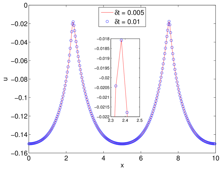
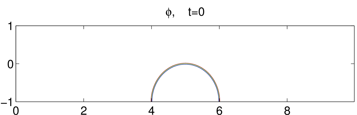
In Fig. 1, we plot the contours of the phase variable at for the two cases, that are obtained using the BDF2 scheme with , , and . We only show the results of the BDF2 scheme since the CN scheme gives visually identical results. In Fig. 2, we plot the -component of velocity at lower boundary for two different time steps and obtained from the BDF2 scheme and CN scheme for the case 2 at . We observe that the results obtained by two schemes are almost identical, which means the time step is small enough to provide very accurate results for this test case.

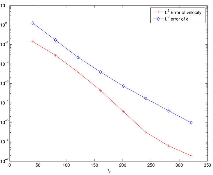
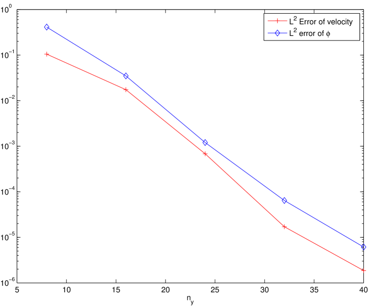
To test the convergence for spatial discretization, we use a very small time step so that the errors from the temporal discretization are negligible compared with the spatial discretization errors. Fig. 3 (a) shows the convergence in -direction, where we fix the number of Legendre modes and vary the number of Fourier modes starting from with the increment . The errors of the velocity field and phase variable are calculated at time , with a reference solution obtained using the finest resolution of . Similarly, Fig. 3 (b) shows the convergence in -direction, where we fix the number of Fourier modes for a series of starting from with an increment . The errors of the velocity field and phase variable are again calculated at with the reference solution using the finest resolutions of and . We see that the proposed numerical schemes can achieve spectral accuracy in norm for both velocity and phase variable.
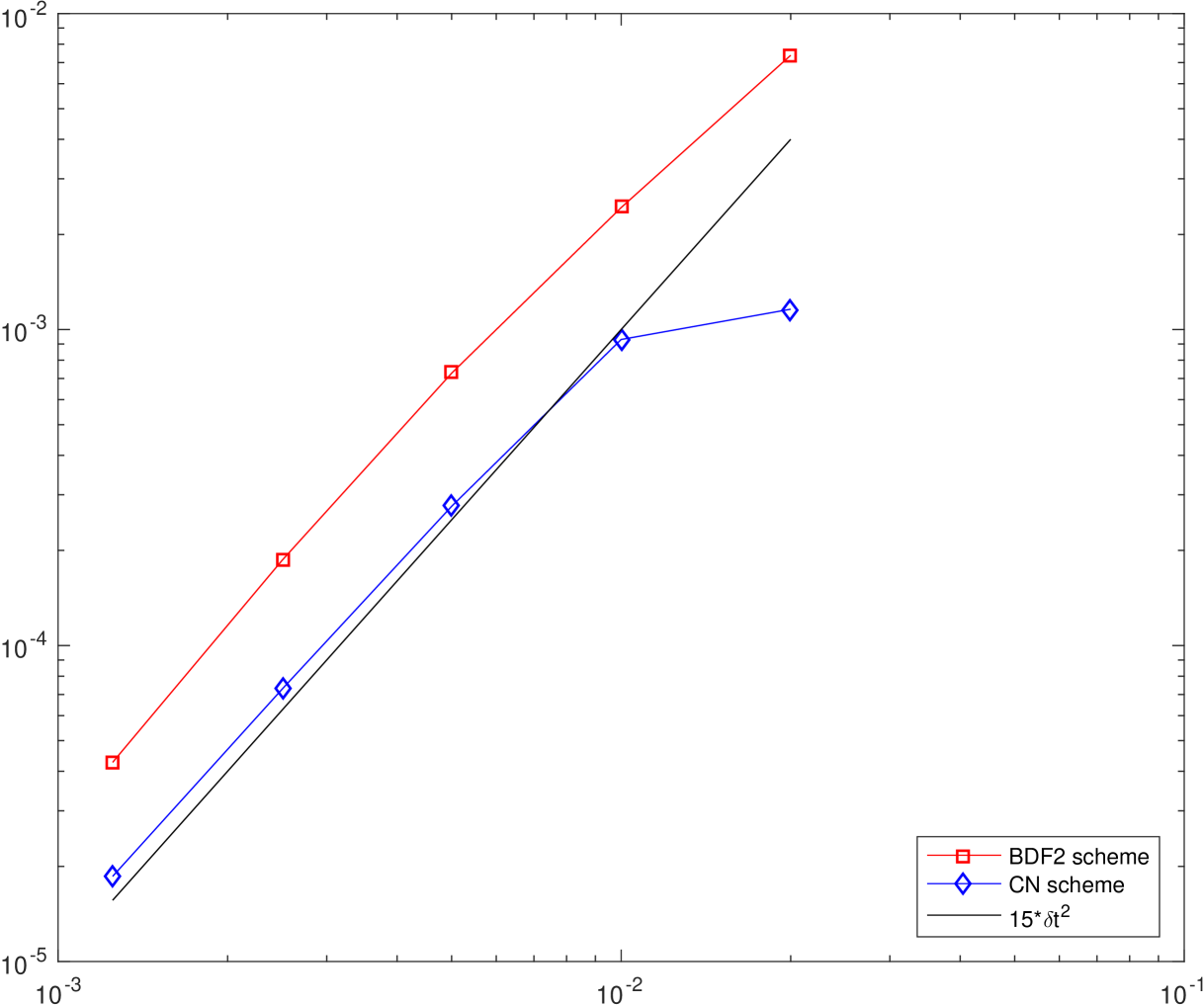
To test the convergence for temporal discretization, we fix the spatial resolution as so that the errors from the spatial discretization are negligible compared to the temporal discretization errors, and perform the refinement test of the time step for the schemes CN and BDF2. We choose the approximate solution using the scheme BDF2 with time step size as the benchmark solution (approximately the exact solution) for computing errors. In Fig. 4, we present the errors of the velocity field and the phase field variable between the numerical solution and the exact solution at with different time step sizes , . The results obtained by CN and BDF2 schemes are shown together with the results obtained by the first order linear stabilization scheme (denoted by LSS) proposed in [46] for comparisons. We observe that both CN and BDF2 schemes are second order accurate for the velocity field as well as the phase field variable , which provide much more accurate results than that of the first order LSS scheme. From Fig. 4, we also observe that the accuracy of CN scheme is better than the accuracy of BDF2 scheme, which is reasonable since CN scheme has a smaller truncation error.
5.2 Energy dissipation and volume preservation
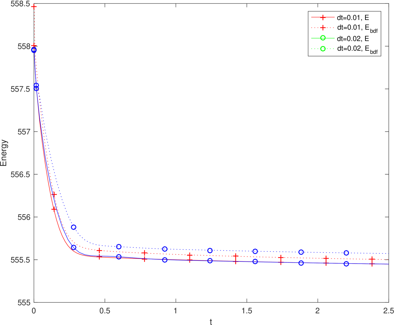
For both CN and BDF2 schemes, we test the energy dissipation for the isolated system by setting the wall velocity , and further compare the evolution of the free energy functional for four different time step sizes where and for the default parameters (5.106) until in Fig. 5. For either scheme, we observe that all energy curves show the decays, that confirm that our algorithms are unconditionally stable. For smaller time steps of , the three energy curves coincide very well. But for the larger time step of , the energy curve is considerable (but not very far) away from others. This means the time step size has to be smaller than in order to get reasonably good accuracy.
To investigate the error introduced by the numerical approximation of (3.22), we plot the IEQ energy and the original energy for the BDF2 scheme using two larger time step sizes and in the left part of Fig. 6. We see that the original energy still have a very good dissipation property, although the differences between the original energy and the IEQ energy are not very small. To further verify the convergence of the difference between the original energy and the modified IEQ energy, we plot in the second part of Fig. 6 the quantity (which is the major part of the difference between the original and IEQ energy) at for both BDF2 scheme and CN scheme using different time steps. A clearly second order convergence is observed.
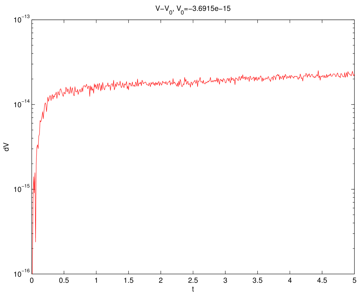
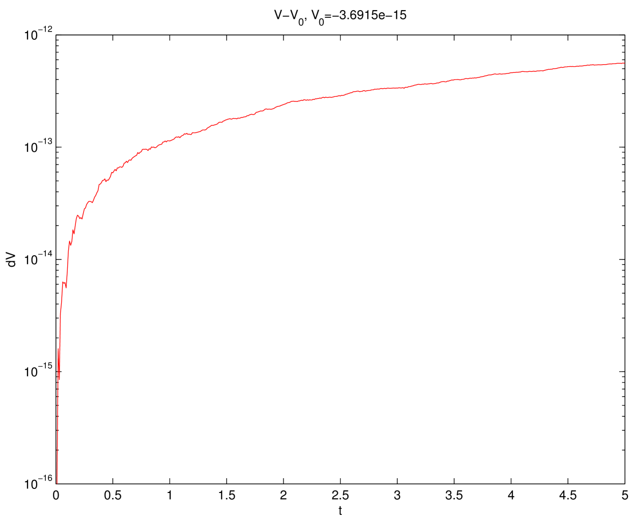
In Fig.7, we show the time evolution for the volume difference where and for the numerical solutions obtained by the schemes CN and BDF2, we observe that the volume difference is very close to the machine precision.
5.3 Efficiency
In Table 1 and Table 2, we show the number of iterations needed by the BiCGSTAB solver for the CN and BDF2 schemes. The default parameters are , , , . We vary these parameters one by one while fixing the rest of them to be default values. In Table 1, the number of iterations are always around for various grid points and , that means the number of iterations actually does not show any dependence on the number of spatial grid points and the parameter . In Table 2, when we vary the time step and parameter , we can see that larger values of them can cause significant increase for the number of iterations. Namely, when and are larger, the conditional numbers of the linear system become worse that is reasonable and can be easily observed from the form of the linear system (3.51).
| 12916 | 25732 | 51364 | |
|---|---|---|---|
| CN | 8 | 8.7 | 9.6 |
| BDF2 | 8.5 | 8.5 | 8.5 |
| 100 | 10 | 1 | |
|---|---|---|---|
| CN | 7.9 | 9 | 9 |
| BDF2 | 9.1 | 10.0 | 10.1 |
| 0.001 | 0.1 | 1 | |
|---|---|---|---|
| CN | 3.8 | 27 | 68 |
| BDF2 | 4 | 27 | 69.6 |
| 1 | 60 | 144 | |
|---|---|---|---|
| CN | 5 | 19.6 | 35.5 |
| BDF2 | 5 | 20.8 | 42.5 |
5.4 Simulation of a drop in shear flow
In this subsection, we simulate the dynamics of a drop in shear flow using BDF2 scheme. The channel length . The wall velocity . All other parameters are given in (5.106).
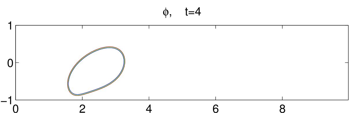
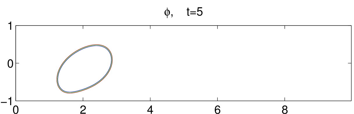
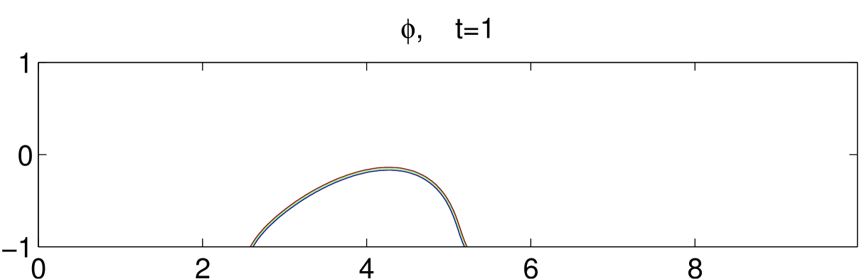
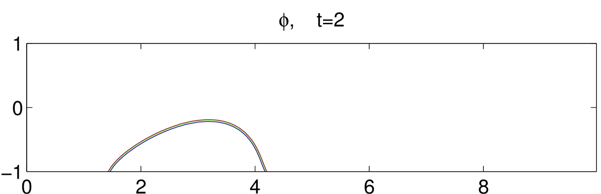
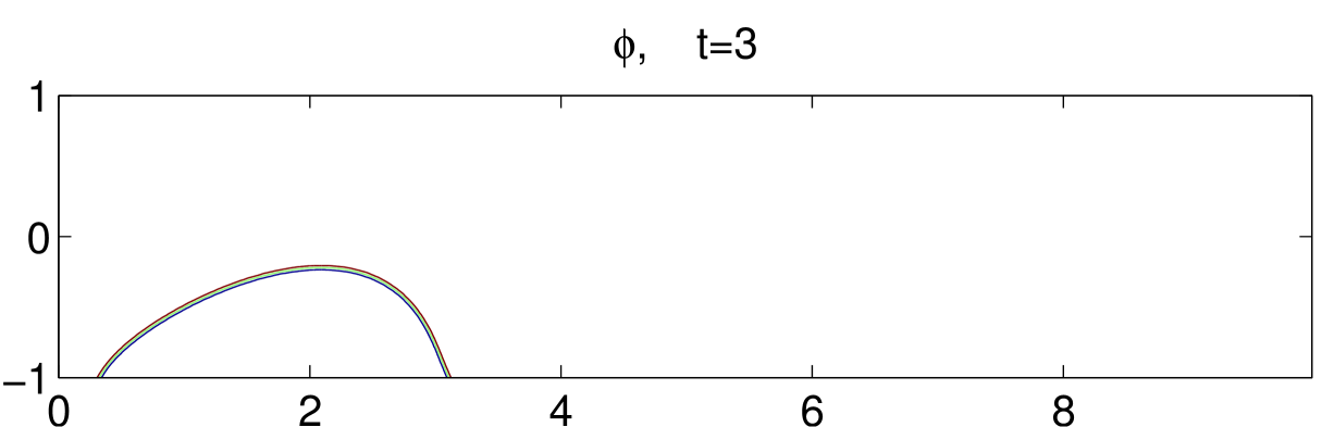
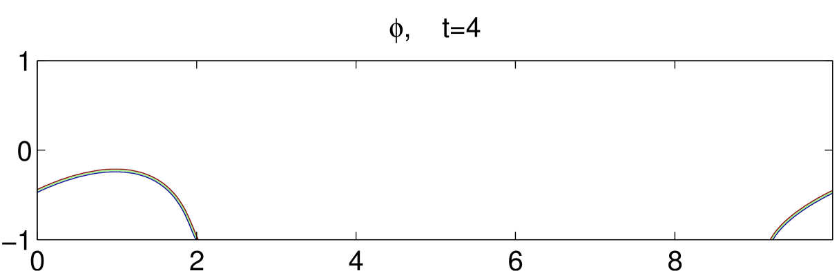
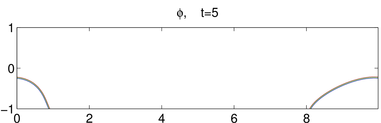
Fig. 8 illustrates the dynamical motions of a drop under shear with an acute contact angle until . Initially, the drop is set in the middle of the bottom plate, as shown in the first subfigure. As the bottom plate moves, the drop also moves with the plate but at a much smaller velocity. This means the drop slips on the bottom plate. As time goes on, the contact region of the drop with the bottom boundary gets smaller and smaller. It eventually gets off the bottom boundary around and moves toward the center of the channel. We also simulate an obtuse contact angle case, in which the drop is harder to get off the bottom boundary. The result is shown in Fig. 9.

6 Concluding remarks
By combining the projection method for Navier-Stokes equations, the IEQ method for the nonlinear bulk and boundary energy gradients, and a subtle explicit-implicit technique for the stress and convective terms, we have constructed two linear, second order unconditionally stable temporal discretization schemes for the phase field MCL model. The well-posedness of the semi-discretized linear systems and their energy stabilities are proved rigorously. Numerical simulations have also verified both schemes are unconditionally stable and second order accurate, while the CN scheme behaves a little bit better than the BDF2 scheme. Although we have considered only time discretizations here, the results can carry over to any consistent finite-dimensional Galerkin (finite element or spectral) approximations since the proofs are all based on variational formulations with all test functions in the same space as the trial function.
Acknowledgments
The work of X. Yang was partially supported by the National Science Foundation under grant number NSF DMS-1418898 and DMS-1720212. The work of H. Yu was partially supported by NSFC projects 11771439, 91530322 and China National Program on Key Basic Research Project 2015CB856003.
References
- [1] S. Aland and F. Chen. An efficient and energy stable scheme for a phase-field model for the moving contact line problem. Int. J. Num. Meth. Fluids., 81:657–671, 2015.
- [2] J. W. Cahn and J. E. Hilliard. Free energy of a nonuniform system. I. interfacial free energy. J. Chem. Phys., 28:258–267, 1958.
- [3] R. Chen, G. Ji, X. Yang, and H. Zhang. Decoupled energy stable schemes for phase-field vesicle membrane model. J. Comput. Phys., 302:509–523, 2015.
- [4] S. Dong. On imposing dynamic contact-angle boundary conditions for wall-bounded liquid-gas flows. Comput. Meth. Appl. Mech. Engrg., 247-248:179–200, 2012.
- [5] S. Dong and J. Shen. A time-stepping scheme involving constant coefficient matrices for phase-field simulations of two-phase incompressible flows with large density ratios. J. Comput. Phys., 231(17):5788–5804, 2012.
- [6] E. B. Dussan. On the spreading of liquids on solid surfaces: Static and dynamic contact lines. Ann. Rev. Fluid Mech., 11(1):371–400, 1979.
- [7] E. B. Dussan and S. H. Davis. On the motion of a fluid-fluid interface along a solid surface. J. Fluid. Mech., 65(01):71–95, 1974.
- [8] W. E and J-G. Liu. Projection method. I. Convergence and numerical boundary layers. SIAM J. Numer. Anal., 32(4):1017–1057, 1995.
- [9] D. J. Eyre. Unconditionally gradient stable time marching the Cahn-Hilliard equation. In Computational and mathematical models of microstructural evolution (San Francisco, CA, 1998), volume 529 of Mater. Res. Soc. Sympos. Proc., pages 39–46. MRS, 1998.
- [10] J. J. Feng, C. Liu, J. Shen, and P. Yue. An energetic variational formulation with phase field methods for interfacial dynamics of complex fluids: advantages and challenges. IMA volumes in Mathematics and Applications, 140:1–26, 2005.
- [11] X. Feng and A. Prohl. Numerical analysis of the Allen–Cahn equation and approximation for mean curvature flows. Numer. Math., 94:33–65, 2003.
- [12] M. Gao and X-P. Wang. A gradient stable scheme for a phase field model for the moving contact line problem. J. Comput. Phys., 231(4):1372–1386, 2012.
- [13] M. Gao and X-P. Wang. An efficient scheme for a phase field model for the moving contact line problem with variable density and viscosity. J. Comput. Phys., 272:704–718, 2014.
- [14] J. L. Guermond, P. Minev, and J. Shen. An overview of projection methods for incompressible flows. Comput. Meth. Appl. Mech. Engrg., 195:6011–6045, 2006.
- [15] J. L. Guermond and J. Shen. On the error estimates for the rotational pressure-correction projection methods. Mathematics of Computation, 73(248):1719–1738, 2004.
- [16] F. Guillén-González and G. Tierra. On linear schemes for a Cahn-Hilliard diffuse interface model. J. Comput. Phys., 234:140–171, 2013.
- [17] D. Han, A. Brylev, X. Yang, and Z. Tan. Numerical analysis of second order, fully discrete energy stable schemes for phase field models of two phase incompressible flows. J. Sci. Comput., 70:965–989, 2017.
- [18] D. Han and X. Wang. A second order in time, uniquely solvable, unconditionally stable numerical scheme for Cahn-Hilliard-Navier-Stokes equation. J. Comput. Phys., 290:139–156, 2015.
- [19] Q. He, R. Glowinski, and X-P. Wang. A least-squares/finite element method for the numerical solution of the Navier–Stokes-Cahn–Hilliard system modeling the motion of the contact line. J. Comput. Phys., 230(12):4991–5009, 2011.
- [20] J. Hua, P. Lin, C. Liu, and Q. Wang. Energy law preserving c0 finite element schemes for phase field models in two-phase flow computations. J. Comput. Phys., 230:7155–7131, 2011.
- [21] J. Kim and J. Lowengrub. Phase field modeling and simulation of three-phase flows. Interfaces Free Bound., 7:435–466, 2005.
- [22] J. Koplik, J. R. Banavar, and J. F. Willemsen. Molecular dynamics of Poiseuille flow and moving contact lines. Phys. Rev. Lett., 60(13):1282–1285, 1988.
- [23] J. Koplik, J. R. Banavar, and J. F. Willemsen. Molecular dynamics of fluid flow at solid surfaces. Phys. Fluids A, 1:781–794, 1989.
- [24] D. Li and Z. Qiao. On Second Order Semi-implicit Fourier Spectral Methods for 2d Cahn–Hilliard Equations. J. Sci. Comput, 70(1):301–341, January 2017.
- [25] D. Li, Z. Qiao, and T. Tang. Characterizing the Stabilization Size for Semi-Implicit Fourier-Spectral Method to Phase Field Equations. SIAM J. Numer. Anal., 54(3):1653–1681, January 2016.
- [26] J. Li and Q. Wang. Mass conservation and energy dissipation issue in a class of phase field models for multiphase fluids. J. Appl. Mech., 81(2):021004, 2013.
- [27] C. Liu and J. Shen. A phase field model for the mixture of two incompressible fluids and its approximation by a Fourier-spectral method. Physica D, 179(3-4):211–228, 2003.
- [28] C. Liu, J. Shen, and X. Yang. Decoupled energy stable schemes for a phase-field model of two-phase incompressible flows with variable density. J. Sci. Comput., 62:601–622, 2015.
- [29] L. Ma, R. Chen, X. Yang, and H. Zhang. Numerical approximations for Allen-Cahn type phase field model of two-phase incompressible fluids with moving contact lines. Comm. Comput. Phys., 21:867–889, 2017.
- [30] C. Miehe, M. Hofacker, and F. Welschinger. A phase field model for rate-independent crack propagation: Robust algorithmic implementation based on operator splits. Comput. Meth. Appl. Mech. Engrg., 199:2765–2778, 2010.
- [31] S. Minjeaud. An unconditionally stable uncoupled scheme for a triphasic Cahn–Hilliard/Navier–Stokes model. Numer. Meth. Part. D. E., 29:584–618, 2013.
- [32] H. K. Moffatt. Viscous and resistive eddies near a sharp corner. J. Fluid Mech., 18(01):1–18, 1964.
- [33] R. H. Nochetto, A. J. Salgado, and I. Tomas. A diffuse interface model for two-phase ferrofluid flows. Comput. Meth. Appl. Mech. Engrg., 309:497–531, 2016.
- [34] T. Qian, X-P. Wang, and P. Sheng. Molecular scale contact line hydrodynamics of immiscible flows. Phys. Rev. E., 68(1):016306, 2003.
- [35] T. Qian, X-P. Wang, and P. Sheng. A variational approach to moving contact line hydrodynamics. J. Fluid Mech., 564:333–360, 2006.
- [36] A. J. Salgado. A diffuse interface fractional time-stepping technique for incompressible two-phase flows with moving contact lines. ESAIM: M2NA, 47:743–769, 2013.
- [37] J. Shen. Efficient spectral-galerkin method I. direct solvers of second- and fourth-order equations using Legendre polynomials. SIAM J. Sci. Comput., 15(6):1489, 1994.
- [38] J. Shen. On error estimates of the projection methods for the Navier-Stokes equations: second-order schemes. Math. Comp., 65(215):1039–1065, 1996.
- [39] J. Shen, C. Wang, S. Wang, and X. Wang. Second-order convex splitting schemes for gradient flows with ehrlich-schwoebel type energy: application to thin film epitaxy. SIAM. J. Numer. Anal., 50:105–125, 2012.
- [40] J. Shen, J. Xu, and J. Yang. A new class of efficient and robust energy stable schemes for gradient flows. arXiv:1710.01331, October 2017.
- [41] J. Shen, J. Xu, and J. Yang. The scalar auxiliary variable (SAV) approach for gradient flows. J. Comput. Phys., 353:407–416, 2017.
- [42] J. Shen and X. Yang. Numerical approximations of Allen–Cahn and Cahn–Hilliard equations. Disc. Cont. Dyn. Sys. A, 28:1669–1691, 2010.
- [43] J. Shen and X. Yang. A phase-field model and its numerical approximation for two-phase incompressible flows with different densities and viscositites. SIAM J. Sci. Comput., 32:1159–1179, 2010.
- [44] J. Shen and X. Yang. Decoupled energy stable schemes for phase filed models of two phase complex fluids. SIAM J. Sci. Comput., 36:B122–B145, 2014.
- [45] J. Shen and X. Yang. Decoupled, energy stable schemes for phase-field models of two-phase incompressible flows. SIAM J. Num. Anal., 53(1):279–296, 2015.
- [46] J. Shen, X. Yang, and H. Yu. Efficient energy stable numerical schemes for a phase field moving contact line model. J. Comput. Phys., 284:617–630, 2015.
- [47] J. Shin, Y. Choi, and J. Kim. An unconditionally stable numerical method for the viscous Cahn–Hilliard equation. Disc. Cont. Dyn. Sys. B, 19:1734–1747, 2014.
- [48] P. Sun, C. Liu, and J. Xu. Phase field model of thermo-induced marangoni effects in the mixtures and its numerical simulations with mixed finite element methods. Comm. Comput. Phys., 6:1095–1117, 2009.
- [49] P. A. Thompson and M. O. Robbins. Simulations of contact-line motion: Slip and the dynamic contact angle. Phys. Rev. Lett., 63(7):766–769, 1989.
- [50] L. J. P. Timmermans, P. D. Minev, and F. N. Van De Vosse. An Approximate Projection Scheme for Incompressible Flow Using Spectral Elements. Int. J. Numer. Meth. Fluids, 22(7):673–688, April 1996.
- [51] J. van Kan. A second-order accurate pressure-correction scheme for viscous incompressible flow. SIAM J. Sci. Statist. Comput., 7(3):870–891, 1986.
- [52] C. Wang and S. M. Wise. An energy stable and convergent finite-difference scheme for the modified phase field crystal equation. SIAM J. Numer. Anal., 49:945–969, 2011.
- [53] L. Wang and H. Yu. Two efficient second order stabilized semi-implicit schemes for the Cahn-Hilliard phase-field equation. arXiv:1708.09763 [math], August 2017. arXiv: 1708.09763.
- [54] C. Xu and T. Tang. Stability analysis of large time-stepping methods for epitaxial growth models. SIAM J. Num. Anal., 44:1759–1779, 2006.
- [55] X. Yang. Linear, first and second order and unconditionally energy stable numerical schemes for the phase field model of homopolymer blends. J. Comput. Phys., 327:294–316, 2016.
- [56] X. Yang, J. J. Feng, C. Liu, and J. Shen. Numerical simulations of jet pinching-off and drop formation using an energetic variational phase-field method. J. Comput. Phys., 218:417–428, 2006.
- [57] X. Yang and D. Han. Linearly first- and second-order, unconditionally energy stable schemes for the phase field crystal equation. J. Comput. Phys., 330:1116–1134, 2017.
- [58] X. Yang and L. Ju. Efficient linear schemes with unconditionally energy stability for the phase field elastic bending energy model. Comput. Meth. Appl. Mech. Engrg., 315:691–712, 2017.
- [59] X. Yang and J. Lu. Linear and unconditionally energy stable schemes for the binary fluid-surfactant phase field model. Comput. Meth. Appl. Mech. Engrg., 318:1005–1029, 2017.
- [60] X. Yang, J. Zhao, and Q. Wang. Numerical approximations for the molecular beam epitaxial growth model based on the invariant energy quadratization method. J. Comput. Phys., 333:104–127, 2017.
- [61] X. Yang, J. Zhao, Q. Wang, and J. Shen. Numerical approximations for a three components Cahn–Hilliard phase-field model based on the invariant energy quadratization method. Mathe. Models and Methods in Appl. Sci., 27:1993–2030, 2017.
- [62] H. Yu and X. Yang. Decoupled energy stable schemes for phase field model with contact lines and variable densities. J. Comput. Phys., 334:665–686, 2017.