Efficient space-time discretizations for tracking the boundaries of reachable sets

Janosch Rieger Kyria Wawryk

Abstract

The reachable sets of nonlinear control systems can in general only be numerically approximated, and are often very expensive to calculate. In this paper, we propose an algorithm that tracks only the boundaries of the reachable sets and that chooses the temporal and spatial discretizations in a non-uniform way to reduce the computational complexity.

Mathematics Subject Classification: 93B03, 65L50.

Keywords: Reachable sets of control systems; Numerical approximation; Boundary tracking; Efficient discretization; Euler’s method.

1 Introduction

The reachable set of a control system represents all possible states the system can attain at a given time. Reachable sets have applications in several different fields, which are often, but not always, related to safety and security [5, 6, 13]. Since explicit formulas for reachable sets are not usually available, we instead must rely on numerical approximation. These approximations are expensive to compute as they need to track an entire set that evolves according to a multivalued flow. In particular, they require a spatial discretization of the set as well as a temporal discretization of the dynamics.

The numerical methods for the computation of reachable sets are split into those which are designed specifically for linear control systems, and those which are applicable to nonlinear systems.

The reachable sets of linear systems are convex and behave in a rather straightforward way. This enables the creation of numerical methods which are theoretically robust and perform well in practice, taking advantage of the fact that the sets can be approximated by relatively simple shapes such as zonotopes [1, 7, 19] or ellipsoids [10], or by a finite number of support points [2, 11].

The shape and behavior of reachable sets of nonlinear control systems is more complex, and so it is unclear how they can be discretized and evolved in the most efficient way. For this reason, several different families of numerical methods have been proposed.

One such family applies the linear methods discussed above to local linearizations of nonlinear systems. Due to the linearization errors, the performance of these methods can depend on the degree of their nonlinearity (see [18] for an analysis).

Another family of algorithms, which are based on optimal control [3, 14], can significantly improve practical performance at the expense of losing guaranteed convergence. These methods use solvers for optimal control problems to approximate the reachable set at a particular time, and thus eliminate the need for spatial discretization at intermediate timesteps at the risk of getting caught in local minima and losing a significant part of the set.

Finally, Runge-Kutta methods for nonlinear differential equations can be generalized to reachable set approximation. Typically, first-order methods are used, as even second-order convergence has prohibitively strict requirements on the control system [20, 21]. Spatial discretization for these methods generally involves representing the reachable set as a subset of a grid [4, 9]. Since these subsets can become very large, storage and computational cost can be reduced by an intelligent choice of discretization [17], or by considering only the boundaries of the reachable sets [15].

In this paper, we aim to combine the benefits of the algorithms proposed in [15] and [17] in a new numerical method for reachable set computation. The boundary tracking algorithm from [15] is essentially a fully discretized set-valued Euler scheme, but it reduces computational complexity by evolving only the boundary of the reachable set in time, and evaluating only the boundary of the multivalued vector field of the control system. The adaptive refinement strategy pursued in [17] aims to identify a space-time discretization with a given a priori error tolerance that minimizes the computational cost of the set-valued Euler scheme. To develop an algorithm that possesses both advantages, we proceed as follows.

After setting our notation and introducing reachable sets and their Euler approximations in Sections 2 and 3, we first have to overcome two technical obstacles in Section 4: The boundary tracking algorithm as published in [15] stores boundaries of discrete reachable sets in an ad-hoc fashion, without exploring the space of all such boundaries from a theoretical perspective. In order to take the algorithm further, we must do so now, and embed it into the framework of [16] for working with boundaries of discrete sets. Furthermore, it turns out that a naive generalization of the algorithm to nonuniform meshes fails, and we introduce appropriate modifications.

In Section 5, we develop an abstract scheme that refines a given space-time discretization until a prescribed error tolerance is met. It is a greedy algorithm in the sense that every refinement step subdivides the time interval where the quotient of the decrease in error and the increase in computational cost is maximized. In Section 6, we derive a concrete estimator for the computational cost of the boundary tracking algorithm for nonuniform discretizations, and prove that it meets the requirements of the abstract refinement scheme. The resulting algorithm is conceptually similar to the method from [17]. It alternates between computing approximate boundaries of the reachable sets for a given space-time discretization and, based on this knowledge of their geometry, refining the mesh. We demonstrate that this process converges in finite time.

Finally, we present two numerical examples in Section 7, which suggest that our algorithm has the potential to outperform the Euler scheme with uniform discretization from [4], the boundary tracking algorithm with uniform discretization from [15] and the Euler scheme with adaptive discretization from [17].

We consciously break away from the tradition to keep algorithms close to the position in the document where they are mentioned. Instead, we display them grouped together on pages 1 to 4, which allows the reader to retrace how the building blocks of the overall algorithm communicate.

2 Notation

We denote $\mathbb{N}_{0}:=\{0,1,2,\ldots\}$ , $\mathbb{N}_{1}=\{1,2,3,\ldots\}$ , $\mathbb{N}_{2}=\{2,3,4,\ldots\}$ and $\mathbb{Z}:=\{\ldots-1,0,1,\ldots\}$ . When $J\subset\mathbb{R}$ is an interval, and when it is clear that $k\in\mathbb{N}$ or $k\in\mathbb{Z}$ , we will write $k\in J$ instead of $k\in J\cap\mathbb{N}$ or $k\in J\cap\mathbb{Z}$ . In addition to the usual $d$ -dimensional vector space $\mathbb{R}^{d}$ , we introduce the space

\mathbb{R}^{0,d}:=\{(x_{0},x_{1},\ldots,x_{d}):x_{0},x_{1},\ldots,x_{d}\in\mathbb{R}\}

and define the cumulative sum $\Sigma_{+}:\mathbb{R}^{d}\to\mathbb{R}^{0,d}$ by $\left(\Sigma_{+}x\right)_{k}:=\sum_{j=1}^{k}x_{j}$ for all $k\in[0,d]$ . We also denote

\mathbb{R}_{+}^{d}:=\{x\in\mathbb{R}^{d}:x_{i}\geq 0\ \forall\,i\in[1,d]\},\quad\mathbb{R}_{>0}^{d}:=\{x\in\mathbb{R}^{d}:x_{i}>0\ \forall\,i\in[1,d]\},

and we extend this notation to $\mathbb{R}^{0,d}$ in the obvious way. We equip $\mathbb{R}^{d}$ with

\|\cdot\|_{\infty}:\mathbb{R}^{d}\to\mathbb{R}_{+}\quad\text{given by}\quad\|x\|_{\infty}:=\max_{i\in[1,d]}|x_{i}|,

and we define the ball with center $x\in\mathbb{R}^{d}$ and radius $r>0$ by

B_{r}(x):=\{y\in\mathbb{R}^{d}:\|x-y\|_{\infty}\leq r\}.

The cardinality of a set $M\subset\mathbb{R}^{d}$ is denoted $\#M$ , and its boundary $\partial M$ .

Let $\mathcal{K}(\mathbb{R}^{d})$ and $\mathcal{KC}(\mathbb{R}^{d})$ denote the collections of all nonempty and compact subsets of $\mathbb{R}^{d}$ , and all nonempty, compact and convex subsets of $\mathbb{R}^{d}$ , respectively. The Hausdorff distance $\operatorname{dist}_{H}:\mathcal{K}(\mathbb{R}^{d})\times\mathcal{K}(\mathbb{R}^{d})\to\mathbb{R}_{+}$ is given by

\operatorname{dist}_{H}(M,\tilde{M})=\max\{\operatorname{dist}(M,\tilde{M}),\,\operatorname{dist}(\tilde{M},M)\},

where

\operatorname{dist}(M,\tilde{M})=\sup_{x\in M}\inf_{\tilde{x}\in\tilde{M}}\|x-\tilde{x}\|_{\infty}.

To approximate $\mathcal{K}(\mathbb{R}^{d})$ , for every $\rho>0$ , we consider the grid $\Delta_{\rho}:=\rho\mathbb{Z}^{d}$ and the collections of digital images

S_{\rho}:=\{M\subset\Delta_{\rho}:M\neq\emptyset\}\quad\text{and}\quad S_{\rho}^{+}:=2^{\Delta_{\rho}}.

By $C_{\rho}$ we denote the collection of all sets $M\in S_{\rho}$ , i.e. sets with the property that for any $x,z\in M$ there exists a finite sequence $(y_{k})_{k=0}^{n}$ with $y_{0}=x$ , $y_{n}=z$ and $\|y_{k+1}-y_{k}\|_{\infty}=\rho$ for all $k\in[0,n-1]$ . These are called chain-connected sets in [15, Definition 9] and $8$ -connected sets (in the plane) in [8, Section 2.2.1].

Finally, a set-valued map $F:\mathbb{R}^{d}\to\mathcal{K}(\mathbb{R}^{d})$ is called $L$ -Lipschitz with $L\in\mathbb{R}_{+}$ if

\operatorname{dist}_{H}(F(x),F(y))\leq L\|x-y\|_{\infty}\quad\forall\,x,y\in\mathbb{R}^{d},

and when $M\subset\mathbb{R}^{d}$ , we denote $F(M):=\cup_{x\in M}F(x)$ .

3 Reachable sets and their approximations

In the following, we briefly introduce reachable sets and a common approach to their numerical computation.

3.1 Reachable sets of differential inclusions

We consider the differential inclusion

\dot{x}(t)\in F(x(t))\ \text{for almost every}\ t\in(0,T),\quad x(0)\in X_{0},

(1)

where $X_{0}\in\mathcal{K}(\mathbb{R}^{d})$ is path-connected, and $F:\mathbb{R}^{d}\to\mathcal{KC}(\mathbb{R}^{d})$ is $L$ -Lipschitz and satisfies the uniform bound

\sup_{x\in\mathbb{R}^{d}}\sup_{f\in F(x)}\|f\|_{\infty}\leq P.

(2)

We are interested in the following sets associated with inclusion (1).

Definition 3.1.

The solution set and the reachable sets of inclusion (1) are

	$\displaystyle\mathcal{S}^{F}(T)$	$\displaystyle:=\{x(\cdot)\in W^{1,1}([0,T],\mathbb{R}^{d}):x(\cdot)\ \text{solves inclusion \eqref{eq:ODI}}\},$
	$\displaystyle\mathcal{R}^{F}(t)$	$\displaystyle:=\{x(t):x(\cdot)\in\mathcal{S}^{F}(T)\},\quad t\in[0,T].$

3.2 The Euler scheme for uniform grids

We discretize the space $\mathcal{K}(\mathbb{R}^{d})$ in a way that is similar to outer Jordan digitization, see [8, Definition 2.8].

Lemma 3.2.

For any numbers $\alpha,\rho>0$ with $\alpha\geq\rho/2$ , the mapping

\pi^{\alpha}_{\rho}:\mathcal{K}(\mathbb{R}^{d})\to S_{\rho}\quad\text{given by}\quad\pi^{\alpha}_{\rho}(M):=B_{\alpha}(M)\cap\Delta_{\rho}

is well-defined, and for all path-connected $M\in\mathcal{K}(\mathbb{R}^{d})$ , we have $\pi^{\alpha}_{\rho}(M)\in C_{\rho}$ .

The Euler map approximates the flow of inclusion (1).

Definition 3.3.

For any given $\alpha,h,\rho>0$ , we define the set-valued functions $\phi_{h}:\mathbb{R}^{d}\to\mathcal{KC}(\mathbb{R}^{d})$ and $\Phi_{h,\rho}^{\alpha}:\mathbb{R}^{d}\to S_{\rho}^{+}$ by

\displaystyle\phi_{h}(x):=x+hF(x)\quad\text{and}\quad\Phi_{h,\rho}^{\alpha}(x):=\pi^{\alpha}_{\rho}(\phi_{h}(x)).

The following proposition is nearly identical to [15, Proposition 12] and is essential for the boundary tracking algorithm to be discussed in Section 4 to work.

Proposition 3.4.

Let $h,\rho>0$ , and define

\alpha(h,\rho):=(1+Lh)\tfrac{\rho}{2}.

(3)

Then for any $M\in C_{\rho}$ and $\alpha\geq\alpha(h,\rho)$ , we have $\Phi_{h,\rho}^{\alpha}(M)\in C_{\rho}$ .

The following Euler scheme for approximating the reachable sets from Definition 3.1 employs a uniform discretization: Every timestep has length $h>0$ , and every point computed is an element of $\Delta_{\rho}$ .

Definition 3.5.

Let $n\in\mathbb{N}_{1}$ , let $\rho>0$ , and let $h:=T/n$ . Then the set of all Euler approximations to inclusion (1) is

\mathcal{S}_{h,\rho}^{F}(T):=\{(y_{k})_{k=0}^{n}:y_{0}\in\pi^{\rho/2}_{\rho}(X_{0}),\ y_{k}\in\Phi^{\alpha(h,\rho)}_{h,\rho}(y_{k-1})\ \forall\,k\in[1,n]\},

and the corresponding approximate reachable sets are

\mathcal{R}_{h,\rho}^{F}(k):=\{y_{k}:(y_{j})_{j=0}^{n}\in\mathcal{S}_{h,\rho}^{F}(T)\},\quad k\in[0,n].

(4)

The discrete solution set $S_{h,\rho}^{F}(T)$ is only used for theoretical purposes. In practice, the discrete reachable sets are computed using the recursion

	$\displaystyle\mathcal{R}_{h,\rho}^{F}(0)$	$\displaystyle=\pi^{\rho/2}_{\rho}(X_{0})$		(5)
	$\displaystyle\mathcal{R}_{h,\rho}^{F}(k)$	$\displaystyle=\Phi^{\alpha(h,\rho)}_{h,\rho}(\mathcal{R}_{h,\rho}^{F}(k-1))\ \forall\,k\in[1,n].$		(5)

Since $X_{0}$ is path-connected, and in view of Lemma 3.2 and Proposition 3.4, we have $\mathcal{R}_{h,\rho}^{F}(k)\in C_{\rho}$ for all $k\in[0,n]$ .

4 Boundary tracking for nonuniform grids

In this section we introduce a storage format for boundaries of digital images, and summarize how the algorithm from [15] tracks the boundaries of the reachable sets from (4). Finally, we show how the restriction operator from [16] helps to overcome technical difficulties that arise when nonuniform discretizations are considered.

4.1 Boundary pairs of digital images

We restate the definition of boundary layers of digital images from [15]. They are related to the so-called distance transform [8, Section 3.4.2].

Definition 4.1.

For every $\rho>0$ and $M\subset\Delta_{\rho}$ , we define

	$\displaystyle\partial_{\rho}^{0}M$	$\displaystyle:=\{x\in M:\exists\,z\in M^{c}\cap\Delta_{\rho}\ \text{with}\ \\|x-z\\|_{\infty}=\rho\},$
	$\displaystyle\partial_{\rho}^{j}M$	$\displaystyle:=\{x\in M^{c}\cap\Delta_{\rho}:\operatorname{dist}(x,\partial_{\rho}^{0}M)=j\rho\},\quad j\in\mathbb{N}_{1},$
	$\displaystyle\partial_{\rho}^{-j}M$	$\displaystyle:=\{x\in M:\operatorname{dist}(x,\partial_{\rho}^{0}M)=j\rho\},\quad j\in\mathbb{N}_{1}.$

The following theorem summarizes the relevant results from [16]:

i)

Every digital image, i.e. every element of $M\in S_{\rho}$ , is uniquely characterized by the pair $(\partial^{0}_{\rho}M,\partial^{1}_{\rho}M)$ .
ii)

There exists a well-defined mapping $\partial R_{\rho}^{\rho^{\prime}}$ that maps the boundary pair of a set $M\in S_{\rho}$ to the boundary pair of a metrically (6) and topologically (7) similar set $R_{\rho}^{\rho^{\prime}}(M)\in S_{\rho^{\prime}}$ that is discretized at a different resolution.

For an illustration of the theorem see the first diagram in Figure 1.

Theorem 4.2.

For every $\rho>0$ , the mapping

\operatorname{Tr}_{\rho}:S_{\rho}\to S_{\rho}^{+}\times S_{\rho}^{+},\quad\operatorname{Tr}_{\rho}(M):=(\partial^{0}_{\rho}M,\partial^{1}_{\rho}M),

is injective, and we write $\operatorname{bd}_{\rho}:=\operatorname{Tr}_{\rho}(S_{\rho})$ and $\operatorname{bdc}_{\rho}:=\operatorname{Tr}_{\rho}(C_{\rho})$ .

For nested grids $\Delta_{\rho^{\prime}}\subsetneq\Delta_{\rho}$ with $\rho^{\prime}\in\rho\mathbb{N}_{2}$ , the operator $R_{\rho}^{\rho^{\prime}}:S_{\rho}\to S_{\rho^{\prime}}$ given by $R_{\rho}^{\rho^{\prime}}(M):=B_{\rho^{\prime}/2}(M)\cap\Delta_{\rho^{\prime}}$ satisfies

	$\displaystyle\forall\,M\in S_{\rho}:\quad\operatorname{dist}_{H}(R_{\rho}^{\rho^{\prime}}(M),M)\leq\rho^{\prime}/2,$			(6)
	$\displaystyle\forall\,M\in C_{\rho}:\quad R_{\rho}^{\rho^{\prime}}(M)\in C_{\rho^{\prime}},$			(7)

and the lifted operator

\partial R_{\rho}^{\rho^{\prime}}:\operatorname{bd}_{\rho}\to\operatorname{bd}_{\rho^{\prime}},\quad\partial R_{\rho}^{\rho^{\prime}}:=\operatorname{Tr}_{\rho^{\prime}}\circ R_{\rho}^{\rho^{\prime}}\circ\operatorname{Tr}_{\rho}^{-1}

(8)

is well-defined.

The mapping $\partial R_{\rho}^{\rho^{\prime}}$ can be implemented efficiently, see [16, Algorithm 1].

4.2 Boundary tracking for uniform grids

In view of Proposition 3.4, the operator

\Psi_{h,\rho}:\operatorname{bdc}_{\rho}\to\operatorname{bdc}_{\rho},\quad\Psi_{h,\rho}(D):=\operatorname{Tr}_{\rho}\circ\,\Phi^{\alpha(h,\rho)}_{h,\rho}\circ\operatorname{Tr}_{\rho}^{-1}(D)

(9)

with $\alpha(h,\rho)$ as in (3) is well-defined. It completes the second diagram in Figure 1. The boundary tracking algorithm from [15] uses $\Psi_{h,\rho}$ to lift recursion (5), which evolves the full reachable sets, to a recursion

	$\displaystyle\operatorname{Tr}_{\rho}(\mathcal{R}_{h,\rho}^{F}(0))$	$\displaystyle=\operatorname{Tr}_{\rho}(\pi^{\rho/2}_{\rho}(X_{0})),$
	$\displaystyle\operatorname{Tr}_{\rho}(\mathcal{R}_{h,\rho}^{F}(k))$	$\displaystyle=\Psi_{h,\rho}(\operatorname{Tr}_{\rho}(\mathcal{R}_{h,\rho}^{F}(k-1)))\quad\forall\,k\in[1,n].$

Since $X_{0}$ is path-connected, it follows from Lemma 3.2 and (9) that

\operatorname{Tr}_{\rho}(\mathcal{R}_{h,\rho}^{F}(k))\in\operatorname{bdc}_{\rho}\quad\forall\,k\in[0,n].

(10)

Figure 1: Mathematically equivalent computations carried out either with entire sets (bottom row) or with their boundaries (top row).

The following theorem is the main result from [15], which allows us to evaluate $\Psi_{h,\rho}(D)$ directly, i.e. without knowledge of $\operatorname{Tr}_{\rho}^{-1}(D)$ . Statement (10) is essential for its proof, which relies on topological arguments.

Theorem 4.3.

Let $h\in(0,\frac{1}{4L}]$ and $\rho>0$ , denote $\alpha=\alpha(h,\rho)$ from (3) and

\kappa=\kappa(h,\rho):=2(1+Lh)(\tfrac{\alpha}{1-Lh}+\rho),

(11)

and let $D=(D_{0},D_{1})\in\operatorname{bdc}_{\rho}$ . Furthermore, consider the set-valued mappings $\phi_{h}^{\partial}:\mathbb{R}^{d}\to\mathcal{K}(\mathbb{R}^{d})$ and $\Phi_{h,\rho}^{\partial,\alpha}:\mathbb{R}^{d}\to S_{\rho}^{+}$ given by

\phi_{h}^{\partial}(x):=\partial\phi_{h}(x)\quad\text{and}\quad\Phi_{h,\rho}^{\partial,\alpha}(x):=\pi_{\rho}^{\alpha}(\phi_{h}^{\partial}(x)),

and the sets

D_{-1}:=\partial_{\rho}^{-1}(\operatorname{Tr}^{-1}(D))\quad\text{and}\quad D_{2}:=\partial_{\rho}^{2}(\operatorname{Tr}^{-1}(D)).

(12)

Then we can form the auxiliary collections

\begin{gathered}W_{0}^{0}:=\Phi^{\partial,\alpha+\kappa}_{h,\rho}(D_{0})\cap\Phi^{\alpha}_{h,\rho}(D_{0}),\quad W_{1}=\Phi^{\partial,\alpha}_{h,\rho}(D_{1}\cup D_{2}),\\ W_{0}^{-1}:=\Phi^{\partial,\alpha}_{h,\rho}(D_{-1}),\end{gathered}

(13)

and we can express $\Psi_{h,\rho}(D)=\tilde{D}$ with the pair $\tilde{D}=(\tilde{D}_{0},\tilde{D}_{1})$ given by

	$\displaystyle\tilde{D}_{1}$	$\displaystyle:=\{x\in W_{1}:\operatorname{dist}(x,W_{0}^{0}\cup W_{0}^{-1})=\rho\},$
	$\displaystyle\tilde{D}_{0}$	$\displaystyle:=\{x\in W_{0}^{0}\cup W_{0}^{-1}:\operatorname{dist}(x,\tilde{D}_{1})=\rho\}$

in terms of $D_{-1},\ D_{0},\ D_{1}$ , and $D_{2}$ .

Theorem 4.3 is the theoretical foundation for Algorithm 1, which is displayed on page 1. Note that it is easy and inexpensive to compute the sets in (12). Figure 2 provides a sketch of the sets used to calculate (13).

(a)

\phi_{h}(x)

(gray), and

\phi_{h}^{\partial}(x)

(dashed)

(b) Blowup required for

x\in D_{0}

x\in D_{k}

k\in\{-1,1,2\}

Figure 2: Sets used in the calculation of

W_{0}^{0},\ W_{0}^{-1}

and

W_{1}

in equations (13) and (18).

4.3 An Euler scheme for nonuniform grids

We present a numerical method that generalizes the Euler scheme from Section 3.2 to nonuniform temporal and spatial discretization parameters

{\bm{\delta}}:=(\bm{h},\bm{t},\bm{\rho})\in\mathbb{R}^{n}_{>0}\times\mathbb{R}_{+}^{0,n}\times\mathbb{R}_{>0}^{0,n},

and is specifically designed to support the boundary tracking algorithm to be proposed in Section 4.4. The vector $\bm{h}=(h_{1},\ldots,h_{n})$ contains stepsizes with $\sum_{k=1}^{n}h_{k}=T$ , the vector $\bm{t}=(t_{0},\ldots,t_{n})=\sum_{+}\bm{h}$ stores the temporal nodes, and the vector $\bm{\rho}=(\rho_{0},\ldots,\rho_{n})$ stores the mesh sizes of the spatial grids $\Delta_{\rho_{0}},\ldots,\Delta_{\rho_{n}}$ associated with the temporal nodes $t_{0},\ldots,t_{n}$ .

The following mapping is to be interpreted as a single Euler step with stepsize $h>0$ and blow-up $\alpha>0$ from the grid $\Delta_{\rho}$ to the grid $\Delta_{\rho^{\prime}}$ . The reason for its particular construction will become apparent in Theorem 4.8.

Definition 4.4.

Let $\alpha,h,\rho,\rho^{\prime}>0$ satisfy $\rho^{\prime}/\rho\in(0,1)\cup\mathbb{N}_{1}$ as well as $\alpha\geq\min(\rho,\rho^{\prime})/2$ . We define the set-valued function $\Phi_{h,\rho,\rho^{\prime}}^{\alpha}:\mathbb{R}^{d}\to S_{\rho^{\prime}}$ by

\Phi_{h,\rho,\rho^{\prime}}^{\alpha}(x):=\begin{cases}R_{\rho}^{\rho^{\prime}}(\Phi_{h,\rho}^{\alpha}(x)),&\rho<\rho^{\prime},\\ \Phi_{h,\rho^{\prime}}^{\alpha}(x),&\rho\geq\rho^{\prime}\end{cases}

with $\Phi_{h,\rho}^{\alpha}$ from Definition 3.3.

Our next result generalizes Proposition 3.4.

Corollary 4.5.

Let $h,\rho,\rho^{\prime}>0$ with $\rho^{\prime}/\rho\in(0,1)\cup\mathbb{N}_{1}$ , and let $\alpha(h,\rho)$ be as in Proposition 3.4. Then for any $M\in C_{\rho}$ , we have $\Phi_{h,\rho,\rho^{\prime}}^{\alpha(h,\rho)}\in C_{\rho^{\prime}}.$

Proof.

When $\rho<\rho^{\prime}$ , then $\Phi_{h,\rho}^{\alpha(h,\rho)}(x)\in C_{\rho}$ by Proposition 3.4, and by statement (7), we have $R_{\rho}^{\rho^{\prime}}(\Phi_{h,\rho}^{\alpha(h,\rho)}(x))\in C_{\rho^{\prime}}$ . If $\rho\geq\rho^{\prime}$ , then $\alpha(h,\rho)\geq\alpha(h,\rho^{\prime})$ , and hence $\Phi_{h,\rho^{\prime}}^{\alpha(h,\rho)}(x)\in C_{\rho^{\prime}}$ directly by Proposition 3.4. ∎

We generalize Definition 3.5 to nonuniform discretizations.

Definition 4.6.

Let $n\in\mathbb{N}_{1}$ , and let ${\bm{\delta}}=(\bm{h},\bm{t},\bm{\rho})\in\mathbb{R}^{n}_{>0}\times\mathbb{R}_{+}^{0,n}\times\mathbb{R}_{>0}^{0,n}$ be such that $\sum_{k=1}^{n}h_{k}=T$ as well as $\bm{t}=\Sigma_{+}\bm{h}$ and $\rho_{k+1}/\rho_{k}\in(0,1)\cup\mathbb{N}_{1}$ for all $k\in[0,n-1]$ . Then the set of all Euler approximations to inclusion (1) is

\mathcal{S}_{\bm{\delta}}^{F}(T):=\{(y_{k})_{k=0}^{n}:y_{0}\in\pi_{\rho_{0}}^{\rho_{0}/2}(X_{0}),\ y_{k}\in\Phi_{h_{k},\rho_{k-1},\rho_{k}}^{\alpha(h_{k},\rho_{k-1})}(y_{k-1})\ \forall\,k\in[1,n]\},

and the discrete approximation to $\mathcal{R}^{F}(t_{k})$ from Definition 3.1 is given by

\mathcal{R}_{\bm{\delta}}^{F}(k):=\{y_{k},y\in\mathcal{S}_{\bm{\delta}}^{F}(T)\},\quad k\in[0,n].

(14)

The proof of the following error bound is very similar to proofs in the literature, see e.g. [4] and [9]. The additive error terms $\chi_{j}({\bm{\delta}})$ occur whenever the operator $R_{\rho_{k}}^{\rho_{k+1}}$ is invoked, see Definition 4.4.

Theorem 4.7.

For any $n\in\mathbb{N}_{1}$ , any ${\bm{\delta}}:=(\bm{h},\bm{t},\bm{\rho})\in\mathbb{R}_{>0}^{n}\times\mathbb{R}_{+}^{0,n}\times\mathbb{R}_{>0}^{0,n}$ satisfying the requirements of Definition 4.6, and any $k\in[0,n]$ , the exact reachable sets of inclusion (1) with property (2) and the discrete reachable sets from Definition 4.6 satisfy

		$\displaystyle\operatorname{dist}_{H}(\mathcal{R}^{F}(t_{k}),\mathcal{R}_{\bm{\delta}}^{F}(k))$		(15)
		$\displaystyle\leq\tfrac{\rho_{0}}{2}e^{Lt_{k}}+\sum_{j=1}^{k}e^{L(t_{k}-t_{j})}[(e^{Lh_{j}}-1)(Ph_{j}+\tfrac{(1+Lh_{j})^{2}}{Lh_{j}}\tfrac{\rho_{j-1}}{2}+\chi_{j}({\bm{\delta}})]$		(15)

for $k\in[0,n]$ , where

\chi_{j}({\bm{\delta}}):=\begin{cases}\tfrac{\rho_{j}}{2},&\rho_{j-1}<\rho_{j},\\ 0,&\text{otherwise}.\end{cases}

As in Section 3.2, the discrete reachable sets (14) satisfy a recursion

	$\displaystyle\mathcal{R}_{\bm{\delta}}^{F}(0)$	$\displaystyle=\pi^{\rho_{0}/2}_{\rho_{0}}(X_{0}),$		(16)
	$\displaystyle\mathcal{R}_{\bm{\delta}}^{F}(k)$	$\displaystyle=\Phi^{\alpha(h_{k},\rho_{k-1})}_{h_{k},\rho_{k-1},\rho_{k}}(\mathcal{R}_{\bm{\delta}}^{F}(k-1))\quad\forall\,k\in[1,n].$		(16)

By Lemma 3.2 and Corollary 4.5, we have $\mathcal{R}_{\bm{\delta}}^{F}(k)\in C_{\rho_{k}}$ for all $k\in[0,n]$ .

4.4 Boundary tracking for nonuniform grids

In view of Corollary 4.5, the mapping

\Psi_{h,\rho,\rho^{\prime}}(D):=\operatorname{Tr}_{\rho^{\prime}}\circ\Phi_{h,\rho,\rho^{\prime}}^{\alpha(h,\rho)}\circ\operatorname{Tr}_{\rho}^{-1}(D)\quad\forall\,D\in\operatorname{bdc}_{\rho}

is an operator $\Psi_{h,\rho,\rho^{\prime}}:\operatorname{bdc}_{\rho}\to\operatorname{bdc}_{\rho^{\prime}}$ . Its action is illustrated in the third diagram in Figure 1. It allows us to lift iteration (16) to the recursion

	$\displaystyle\operatorname{Tr}_{\rho_{0}}(\mathcal{R}_{\bm{\delta}}^{F}(0))$	$\displaystyle=\operatorname{Tr}_{\rho_{0}}(\pi^{\rho_{0}/2}_{\rho_{0}}(X_{0})),$		(17)
	$\displaystyle\operatorname{Tr}_{\rho_{k}}(\mathcal{R}_{{\bm{\delta}}}^{F}(k))$	$\displaystyle=\Psi_{h_{k},\rho_{k-1},\rho_{k}}(\operatorname{Tr}_{\rho_{k-1}}(\mathcal{R}_{\bm{\delta}}^{F}(k-1)))\quad\forall\,k\in[1,n],$		(17)

which is displayed on page 2 as Algorithm 2. Again because of Lemma 3.2, we have $\operatorname{Tr}_{\rho_{k}}(\mathcal{R}_{{\bm{\delta}}}^{F}(k))\in\operatorname{bdc}_{\rho_{k}}$ for all $k\in[0,n]$ . Note that these iterates are the boundary pairs of the sets $\mathcal{R}_{{\bm{\delta}}}^{F}(k)$ which satisfy the error bound (15).

To carry out recursion (17) without knowledge of the set $\mathcal{R}_{h,\rho}^{F}(k-1)$ , we would ideally like to generalize Theorem 4.3 to nonuniform grids. An inspection of its proof, given in [15], shows that the theorem remains valid when $\rho_{k+1}\leq\rho_{k}$ . Elementary counterexamples show, however, that the theorem is false when $\rho_{k+1}>\rho_{k}$ . The construction in Definition 4.4 circumvents this problem, as it allows the representation (19) below.

Theorem 4.8.

Let $h\in(0,\frac{1}{4L}]$ , and let $\rho,\rho^{\prime}>0$ satisfy $\rho^{\prime}/\rho\in(0,1)\cup\mathbb{N}_{1}$ . Let $\alpha=\alpha(h,\rho)$ and $\kappa=\kappa(h,\rho)$ as in (3) and (11), let $\tilde{\rho}:=\min(\rho,\rho^{\prime})$ , and consider a pair $D=(D_{0},D_{1})\in\operatorname{bdc}_{\rho}$ . Denoting

D_{-1}:=\partial_{\rho}^{-1}(\operatorname{Tr}^{-1}(D))\quad\text{and}\quad D_{2}:=\partial_{\rho}^{2}(\operatorname{Tr}^{-1}(D)),

we can form the auxiliary collections

\begin{gathered}W_{0}^{0}:=\Phi^{\partial,\alpha+\kappa}_{h,\tilde{\rho}}(D_{0})\cap\Phi^{\alpha}_{h,\tilde{\rho}}(D_{0}),\quad W_{1}:=\Phi^{\partial,\alpha}_{h,\tilde{\rho}}(D_{1}\cup D_{2}),\\ W_{0}^{-1}:=\Phi^{\partial,\alpha}_{h,\tilde{\rho}}(D_{-1})\end{gathered}

(18)

and the pair $\tilde{D}=(\tilde{D}_{0},\tilde{D}_{1})$ given by $\tilde{D}_{1}:=\{x\in W_{1}:\operatorname{dist}(x,W_{0}^{0}\cup W_{0}^{-1})=\tilde{\rho}\}$ and $\tilde{D}_{0}:=\{x\in W_{0}^{0}\cup W_{0}^{-1}:\operatorname{dist}(x,\tilde{D}_{1})=\tilde{\rho}\}$ . Then we can express

\Psi_{h,\rho,\rho^{\prime}}(D)=\begin{cases}\tilde{D},&\rho^{\prime}\leq\rho,\\ \partial R_{\tilde{\rho}}^{\rho^{\prime}}(\tilde{D}),&\text{else}.\end{cases}

(19)

in terms of $D_{-1}$ , $D_{0}$ , $D_{1}$ and $D_{2}$ , using $\partial R_{\tilde{\rho}}^{\rho^{\prime}}$ from (8).

Proof.

A proof identical to that of Theorem 4.3 shows $\tilde{D}\in\operatorname{bdc}_{\tilde{\rho}}$ and

\displaystyle\Psi_{h,\rho,\tilde{\rho}}(D)=\tilde{D}.

(20)

If $\rho^{\prime}\leq\rho$ , we have $\tilde{\rho}=\rho^{\prime}$ and (20) implies (19). If $\rho^{\prime}>\rho$ , then $\tilde{\rho}=\rho$ and using equation (8), Definition 4.4, and equation (20), we verify statement (19) by the computation

	$\displaystyle\Psi_{h,\rho,\rho^{\prime}}(D)=\operatorname{Tr}_{\rho^{\prime}}\circ\Phi_{h,\rho,\rho^{\prime}}^{\alpha}\circ\operatorname{Tr}_{\rho}^{-1}(D)$
	$\displaystyle=\operatorname{Tr}_{\rho^{\prime}}\circ R_{\rho}^{\rho^{\prime}}\circ\Phi_{h,\rho}^{\alpha}\circ\operatorname{Tr}_{\rho}^{-1}(D)=\operatorname{Tr}_{\rho^{\prime}}\circ R_{\rho}^{\rho^{\prime}}\circ\Phi_{h,\rho,\tilde{\rho}}^{\alpha}\circ\operatorname{Tr}_{\rho}^{-1}(D)$
	$\displaystyle=\partial R_{\rho}^{\rho^{\prime}}\circ\operatorname{Tr}_{\rho}\circ\Phi_{h,\rho,\tilde{\rho}}\circ\operatorname{Tr}^{-1}(D)=\partial R_{\rho}^{\rho^{\prime}}\circ\Psi_{h,\rho,\tilde{\rho}}(D)=\partial R_{\rho}^{\rho^{\prime}}(\tilde{D}).$

∎

Algorithm 1 implements the operator $\Psi_{h,\rho,\rho^{\prime}}$ as proposed in Theorem 4.8. In addition to an image $\Psi_{h,\rho,\rho^{\prime}}(D_{0},D_{1})$ , it returns the numbers $\hat{c}_{R}\in\mathbb{N}_{1}$ and $\hat{c}_{F}\in\mathbb{N}_{1}$ of grid points, which can be counted incidentally and are the key ingredients for the surrogate volumes (42) and (43). An implementation of the operator $\partial R_{\rho}^{\rho^{\prime}}$ , which occurs in line 1, is available in [16, Algorithm 1].

5 An abstract subdivision scheme

The primary contribution of this paper is Algorithm 4, displayed on page 4, which alternates between executing recursion (17) and refining the discretization based on information gathered in the recursion. This section develops an abstract subdivision scheme for the latter aspect, displayed as Algorithm 3 on page 3, which will be applied to concrete cost and error estimators $C$ and $E$ in Section 6.

The following discretizations are admissible for the subdivision process.

Definition 5.1.

By $\aleph_{n}\subset\mathbb{R}_{>0}^{n}\times\mathbb{R}_{+}^{n+1}\times\mathbb{R}_{>0}^{n+1}$ we denote the set of all tuples ${\bm{\delta}}=(\bm{h},\bm{t},\bm{\rho})\in\mathbb{R}_{>0}^{n}\times\mathbb{R}_{+}^{n+1}\times\mathbb{R}_{>0}^{n+1}$ such that

	$\displaystyle\bm{t}=\Sigma_{+}\bm{h},\quad T=t_{n}$		(21)
	$\displaystyle\\|\bm{h}\\|_{\infty}\leq\tfrac{1}{4L},\quad\\|\bm{\rho}\\|_{\infty}\leq\tfrac{P}{8L}$		(22)
	$\displaystyle\tfrac{\rho_{j}}{\rho_{k}}\in\{4^{\ell}:\ell\in\mathbb{Z}\}\quad\forall\,j,k\in[0,n],$		(23)
	$\displaystyle\rho_{j}=2LP\left(h_{j}\right)^{2}\quad\forall\,j\in[1,n],$		(24)

Additionally, we denote

\aleph:=\cup_{n\in\mathbb{N}_{1}}\aleph_{n}.

We will refine a given discretization by repeated subdivision according to the following rule.

Definition 5.2.

Given any $n\in\mathbb{N}_{1}$ and ${\bm{\delta}}=(\bm{h},\bm{t},\bm{\rho})\in\aleph_{n}$ , we define the function

\psi[{\bm{\delta}};j]=\left(\psi_{h}[\bm{h};j],\psi_{t}[\bm{t};j],\psi_{\rho}[\bm{\rho};j]\right)

(25)

given by

$\displaystyle\psi_{h}[\bm{h};j]$	$\displaystyle:=\begin{cases}\bm{h},&j=0,\\ (h_{1},...,h_{j-1},h_{j}/2,h_{j}/2,h_{j+1},...,h_{n}),&j\in[1,n],\end{cases}$	(26)
$\displaystyle\psi_{t}[\bm{t};j]$	$\displaystyle:=\begin{cases}\bm{t},&j=0,\\ (t_{0},...,t_{j-1},t_{j}-h_{j}/2,t_{j},t_{j+1},...,t_{n}),&j\in[1,n],\end{cases}$
$\displaystyle\psi_{\rho}[\bm{\rho};j]$	$\displaystyle:=\begin{cases}(\rho_{0}/4,\rho_{1},...,\rho_{n}),&j=0,\\ (\rho_{0},...,\rho_{j-1},\rho_{j}/4,\rho_{j}/4,\rho_{j+1},...,\rho_{n}),&j\in[1,n].\end{cases}$

Throughout the rest of this section, we consider two functions

C,E:\aleph\to\mathbb{R}_{>0}

that assign a number to every admissible discretization, and the change

	$\displaystyle\Delta C({\bm{\delta}};j):=C(\psi[{\bm{\delta}};j])-C({\bm{\delta}})\quad\forall\,n\in\mathbb{N}_{1},\ \forall\,{\bm{\delta}}\in\aleph_{n},\ \forall\,j\in[0,n],$
	$\displaystyle\Delta E({\bm{\delta}};j):=E(\psi[{\bm{\delta}};j])-E({\bm{\delta}})\quad\forall\,n\in\mathbb{N}_{1},\ \forall\,{\bm{\delta}}\in\aleph_{n},\ \forall\,j\in[0,n]$

in these functions caused by the subdivision rule $\psi$ . We assume that these functions have the following properties:

P1

There exists a function $\omega_{1}\in C^{0}(\mathbb{R}_{>0},\mathbb{R}_{>0})$ such that $\lim_{s\to 0}\omega_{1}(s)=0$ and $E({\bm{\delta}})\leq\omega_{1}(\|\bm{\rho}\|_{\infty})$ holds for all $n\in\mathbb{N}_{1}$ and ${\bm{\delta}}\in\aleph_{n}$ .
P2

There exists a strictly increasing function $\omega_{2}\in C^{0}(\mathbb{R}_{+},\mathbb{R}_{+})$ such that $\omega_{2}(0)=0$ and $\Delta E({\bm{\delta}};j)\leq-\omega_{2}(\rho_{j})$ holds for all $n\in\mathbb{N}_{1}$ , all ${\bm{\delta}}\in\aleph_{n}$ and all $j\in[0,n]$ .
P3

We have $\Delta C({\bm{\delta}};\arg\min_{i}\rho_{i})>0$ for all $n\in\mathbb{N}_{1}$ and ${\bm{\delta}}\in\aleph_{n}$ .
P4

There exists $\omega_{4}\in C^{0}(\mathbb{R}_{>0},\mathbb{R}_{>0})$ such that

$\Delta C({\bm{\delta}};j)\leq\omega_{4}(\rho_{j})\Delta C({\bm{\delta}};\arg\min_{i}\rho_{i})$

holds for all $n\in\mathbb{N}_{1}$ , all ${\bm{\delta}}\in\aleph_{n}$ and all $j\in[0,n]$ .

Remark 5.3.

Though it is somewhat counterintuitive, examples show that the differences $\Delta C({\bm{\delta}};j)$ can be negative. For this reason, property P4 does not imply P3.

The following lemma is derived from (25) by a straightforward induction.

Lemma 5.4.

Let $N\in\mathbb{N}_{0}$ , and let the sequences $({\bm{\delta}}^{(m)})_{m=0}^{N}$ , $(k_{m})_{m=0}^{N}$ , and $(n_{m})_{m=0}^{N}$ be generated by Algorithm 3 from ${\bm{\delta}}^{(0)}\in\aleph_{n_{0}}$ . Then ${\bm{\delta}}^{(m)}\in\aleph_{n_{m}}$ for all $m\in[0,N]$ .

If the spatial discretizations generated by Algorithm 3 do not become uniformly arbitrarily fine, then there exists a particular node at which the discretization eventually remains constant.

Lemma 5.5.

Assume that Algorithm 3 does not terminate, and that the sequences $({\bm{\delta}}^{(m)})_{m=0}^{\infty}$ , $(k_{m})_{m=0}^{\infty}$ , and $(n_{m})_{m=0}^{\infty}$ with ${\bm{\delta}}^{(m)}=(\bm{h}^{(m)},\bm{t}^{(m)},\bm{\rho}^{(m)})$ it generates satisfy

\lim_{m\to\infty}\|\bm{\rho}^{(m)}\|_{\infty}\neq 0.

(27)

Then there exist $m_{0}\in\mathbb{N}$ and $j_{m_{0}}\in[0,n_{m_{0}}]$ such that for all $m\in[m_{0},\infty)$ , there exists $j_{m}\in[0,n_{m}]$ with $t_{j_{m}}^{(m)}=t_{j_{m_{0}}}^{(m_{0})}$ and $\rho_{j_{m}}^{(m)}=\rho_{j_{m_{0}}}^{(m_{0})}$ .

Proof.

By statement (26), the sequence $(\|\bm{\rho}^{(m)}\|_{\infty})_{m=0}^{\infty}$ is a monotone decreasing sequence of positive numbers. Hence there exists $s\in\mathbb{R}_{+}$ with $\lim_{m\to\infty}\|\bm{\rho}^{(m)}\|_{\infty}=s$ . By statement (27), we have $s>0$ , and it follows from statement (23) that there exists $m_{0}\in\mathbb{N}$ with

\|\bm{\rho}^{(m)}\|_{\infty}=s\quad\forall\,m\in[m_{0},\infty).

(28)

Hence the sets

S_{m}:=\{t_{j}^{(m)}:j\in[0,n_{m}],\ \rho_{j}^{(m)}=s\},\quad m\in[m_{0},\infty),

are nonempty and closed subsets of the compact set $[0,T]$ . By statements (26) and (28), we also have $S_{m+1}\subset S_{m}$ for all $m\in[m_{0},\infty)$ , so by [12, Theorem 26.9], we have $\cap_{m\in[m_{0},\infty)}S_{m}\neq\emptyset$ , which yields the desired result. ∎

If Algorithm 3 does not terminate, then the event that the currently finest spatial discretization is refined in line 3 occurs infinitely often.

Lemma 5.6.

If Algorithm 3 does not terminate in finite time and generates sequences $({\bm{\delta}}^{(m)})_{m=0}^{\infty}$ , $(k_{m})_{m=0}^{\infty}$ , and $(n_{m})_{m=0}^{\infty}$ with ${\bm{\delta}}^{(m)}=(\bm{h}^{(m)},\bm{t}^{(m)},\bm{\rho}^{(m)})$ , then the set $\mathbb{N}^{\prime}:=\{m\in\mathbb{N}_{1}:\rho_{k_{m}}^{(m)}=\min_{j\in[0,n_{m}]}\rho_{j}^{(m)}\}$ is infinite.

Proof.

Assume that $\mathbb{N}^{\prime}$ is finite, and take $\tilde{m}:=\max(\mathbb{N}^{\prime})+1$ , so that

\rho_{k_{m}}^{(m)}>\min_{j\in[0,n_{m}]}\rho_{j}^{(m)}\quad\forall\,m\in[\tilde{m},\infty).

(29)

We assert by induction that this implies

\tilde{\rho}:=\min_{j\in[0,n_{\tilde{m}}]}\rho_{j}^{(\tilde{m})}=\min_{j\in[0,n_{m}]}\rho_{j}^{(m)}\quad\forall\,m\in[\tilde{m},\infty).

(30)

This is clearly true for $m=\tilde{m}$ . If (30) holds for some $m\in[\tilde{m},\infty)$ , then by (23) and (29), we have $\rho_{k_{m}}^{(m)}\geq 4\min_{j\in[0,n_{m}]}\rho_{j}^{(m)}$ , so by statement (26) we find that (30) holds with $m+1$ in lieu of $m$ .

To derive a contradiction, we introduce the auxiliary function

\beta:[\tilde{m},\infty)\to\mathbb{R},\quad\beta(m):=\log_{4}(\tfrac{\rho_{0}^{(m)}}{\tilde{\rho}})+\sum_{j=1}^{n_{m}}(2^{\log_{4}(\rho_{j}^{(m)}/\tilde{\rho})}-1).

By (30) we have $\rho_{j}^{(m)}\geq\tilde{\rho}$ and hence $\log_{4}(\rho_{j}^{(m)}/\tilde{\rho})\geq 0$ for all $m\in[\tilde{m},\infty)$ and $j\in[0,n_{m}]$ . Together with (23), we obtain that

\log_{4}(\rho_{j}^{(m)}/\tilde{\rho})\in\mathbb{N}_{0}\quad\forall\,m\in[\tilde{m},\infty),\ \forall\,j\in[0,n_{m}],

(31)

and hence that $\beta(m)\in\mathbb{N}_{0}$ for all $m\in[\tilde{m},\infty)$ . Using (26), it is easy to check that

\beta(m+1)=\beta(m)-1,\quad\forall\,m\in[\tilde{m},\infty),

which implies that for $\hat{m}:=\tilde{m}+\beta(\tilde{m})$ , we have $\beta(\hat{m})=0$ . By (31), this forces $\rho^{(\hat{m})}=\tilde{\rho}\mathbbm{1}$ . In particular, we have

\rho^{(\hat{m})}_{k_{\hat{m}}}=\tilde{\rho}=\min_{j\in[0,n_{\hat{m}}]}\rho_{j}^{(\hat{m})},

which implies $\hat{m}\in\mathbb{N}^{\prime}$ . Since $\tilde{m}\leq\hat{m}$ , this contradicts the definition of $\tilde{m}$ . ∎

Now we prove that Algorithm 3 terminates in finite time.

Theorem 5.7.

If the functions $C$ and $E$ satisfy properties P1–P4, then, for any ${\bm{\delta}}^{(0)}\in\aleph_{n_{0}}$ and $\varepsilon>0$ , Algorithm 3 terminates after a finite number $m\in\mathbb{N}$ of iterations and returns a ${\bm{\delta}}^{(m)}\in\aleph_{n_{m}}$ with $E({\bm{\delta}}^{(m)})\leq\varepsilon$ .

Proof.

Assume that Algorithm 3 does not terminate. Then it generates sequences $({\bm{\delta}}^{(m)})_{m=0}^{\infty}$ , $(k_{m})_{m=0}^{\infty}$ and $(n_{m})_{m=0}^{\infty}$ with ${\bm{\delta}}^{(m)}=(\bm{h}^{(m)},\bm{t}^{(m)},\bm{\rho}^{(m)})$ for all $m\in\mathbb{N}$ and

E({\bm{\delta}}^{(m)})>\varepsilon\quad\forall\,m\in\mathbb{N}.

(32)

In the following, we show that

\lim_{m\to\infty}\|\bm{\rho}^{(m)}\|_{\infty}=0,

(33)

which, in conjunction with property P1, contradicts (32). This, combined with Lemma 5.4, completes the proof.

We obtain from property P2 that

\Delta E({\bm{\delta}}^{(m)};j)\leq-\omega_{2}(\rho_{j}^{(m)})<0,\quad\forall\,m\in\mathbb{N}_{1},\ \forall\,j\in[0,n_{m}],

(34)

and by construction, we have

-\sum_{j=0}^{m-1}\Delta E({\bm{\delta}}^{(j)};k_{j})=E({\bm{\delta}}^{(0)})-E({\bm{\delta}}^{(m)})\leq E({\bm{\delta}}^{(0)}),\quad\forall\,m\in\mathbb{N}_{1}.

(35)

Combining (34) and (35) yields

\lim_{m\to\infty}\Delta E({\bm{\delta}}^{(m)};k_{m})=0.

(36)

If statement (33) is false, then by Lemma 5.5, there exist $m_{0}\in\mathbb{N}_{1}$ and $i_{m_{0}}\in[0,n_{m_{0}}]$ such that, for every $m\in[m_{0},\infty)$ , there exists $i_{m}\in[0,n_{m}]$ with

\rho_{i_{m}}^{(m)}=\rho_{i_{m_{0}}}^{(m_{0})}.

(37)

By Lemma 5.6, the set

\mathbb{N}^{\prime}=\{m\in\mathbb{N}_{1}:\rho_{k_{m}}^{(m)}=\min_{j\in[0,n_{m}]}\rho_{j}^{(m)}\}

is infinite, and hence $\mathbb{N}^{\prime\prime}:=[m_{0},\infty)\cap\mathbb{N}^{\prime}$ is infinite as well. By property P3, we have

\Delta C({\bm{\delta}}^{(m)};k_{m})>0\quad\forall\,m\in\mathbb{N}^{\prime\prime}.

(38)

If $\Delta C({\bm{\delta}}^{(m)};j)\leq 0$ for some $m\in\mathbb{N}^{\prime\prime}$ and $j\in[0,n_{m}]$ , then the condition in line 3 of Algorithm 3 is false, and so line 3 yields the contradiction $\Delta C({\bm{\delta}}^{(m)};k_{m})\leq 0$ . Hence

\Delta C({\bm{\delta}}^{(m)};j)>0\quad\forall\,m\in\mathbb{N}^{\prime\prime},\ \forall\,j\in[0,n_{m}],

so line 3 is executed in iteration $m$ for all $m\in\mathbb{N}^{\prime\prime}$ , and thus we have

\tfrac{\Delta E({\bm{\delta}}^{(m)};k_{m})}{\Delta C({\bm{\delta}}^{(m)};k_{m})}\leq\tfrac{\Delta E({\bm{\delta}}^{(m)};i_{m})}{\Delta C({\bm{\delta}}^{(m)};i_{m})}\quad\forall\,m\in\mathbb{N}^{\prime\prime}.

By (34) and (38), by (34) and property P2, by (37), and by (36), we have

	$\displaystyle\lim_{\mathbb{N}^{\prime\prime}\ni m\to\infty}\tfrac{\Delta C({\bm{\delta}}^{(m)};k_{m})}{\Delta C({\bm{\delta}}^{(m)};i_{m})}\leq\lim_{\mathbb{N}^{\prime\prime}\ni m\to\infty}\tfrac{\Delta E({\bm{\delta}}^{(m)};k_{m})}{\Delta E({\bm{\delta}}^{(m)};i_{m})}$
	$\displaystyle\leq\lim_{\mathbb{N}^{\prime\prime}\ni m\to\infty}\tfrac{\Delta E({\bm{\delta}}^{(m)};k_{m})}{-\omega_{2}(\rho_{i_{m}}^{(m)})}=\lim_{\mathbb{N}^{\prime\prime}\ni m\to\infty}\tfrac{\Delta E({\bm{\delta}}^{(m)};k_{m})}{-\omega_{2}(\rho_{i_{m_{0}}}^{(m_{0})})}=0.$

However, in view of the definition of $\mathbb{N}^{\prime\prime}$ , property P4 and (37) provide

\tfrac{\Delta C({\bm{\delta}}^{(m)};k_{m})}{\Delta C({\bm{\delta}}^{(m)};i_{m})}\geq\omega_{4}(\rho^{(m)}_{i_{m}})^{-1}=\omega_{4}(\rho^{(m_{0})}_{i_{m_{0}}})^{-1}>0\quad\forall\,m\in\mathbb{N}^{\prime\prime},

contradicting the above statement. ∎

6 Efficient discretizations for boundary tracking

We wish to measure the quality of a discretization

{\bm{\delta}}=(\bm{h},\bm{t},\bm{\rho})\in\mathbb{R}^{n}_{>0}\times\mathbb{R}_{+}^{0,n}\times\mathbb{R}_{>0}^{0,n}

in terms of the a priori error of the corresponding discrete reachable sets and the cost of their computation. This will allow us to select a discretization with a high benefit-to-cost ratio. To this end, we split the a priori error bound

\displaystyle E({\bm{\delta}})

\displaystyle=\sum_{k=0}^{n}\mathcal{E}_{k}({\bm{\delta}}),

(39)

from Theorem 4.7 for the reachable sets computed in recursion (17) into the contribution $\mathcal{E}_{0}({\bm{\delta}}):=\frac{\rho_{0}}{2}e^{LT}$ from the discretization of the initial set $X_{0}$ and the contributions

\mathcal{E}_{k}({\bm{\delta}}):=e^{L(T-t_{k})}\Big{[}(e^{Lh_{k}}-1)\big{(}Ph_{k}+\tfrac{(1+Lh_{k})^{2}}{Lh_{k}}\tfrac{\rho_{k-1}}{2}\big{)}+\chi_{k}({\bm{\delta}})\Big{]},\ k\in(0,n],

from the discretization of the dynamics on each subinterval $(t_{k-1},t_{k}]$ for $k\in(0,n]$ , where we use the notation

\chi_{k}({\bm{\delta}}):=\begin{cases}\tfrac{\rho_{k}}{2},&\rho_{k-1}<\rho_{k},\\ 0,&\text{otherwise}.\end{cases}

Since there is no straightforward a priori formula for the computational cost of recursion (17) available, we derive a heuristic estimator based on a posteriori knowledge from previously performed computations in Section 6.1. We verify in Section 6.2 that this cost estimator and the a priori error estimate (39) satisfy properties P1 to P4, which means that it is safe to carry out the subdivision scheme from Section 5 with these particular inputs.

6.1 Estimating the computational cost

We first collect some preliminaries:

Recall that $d$ is the dimension of the state space, and let

d_{x}:=\max_{t\in[0,T]}\dim\mathcal{R}^{F}(t)\quad\text{and}\quad d_{u}:=\max_{t\in[0,T]}\max_{x\in\mathcal{R}^{F}(t)}\dim F(x).

Then the numbers

d_{R}:=\min(d-1,d_{x})\quad\text{and}\quad d_{F}:=\min(d-1,d_{u})

are a good guess for the dimension of the boundary of the reachable sets and the boundary of the right-hand side $F$ , see Figure 3 for an illustration. From here forward, we assume that $d_{R}\geq 1$ to rule out pathological situations.

ii)

We express the average thickness of the generalized annuli computed in the evaluation of the operator $\Psi_{h,\rho,\rho^{\prime}}$ in line 1 of Algorithm 1 and (18), respectively, in terms of the function $\sigma:(0,\tfrac{1}{4L}]\times(0,\tfrac{P}{8L}]\to\mathbb{R}_{>0}$ given by

\sigma(h,\rho):=2\alpha(h,\rho)+\tfrac{1}{4}\kappa(h,\rho)=\tfrac{\rho}{4}(1+Lh)\left(\tfrac{1+Lh}{1-Lh}+6\right).

(40)

Figure 2 on page 2 provides a visualization of these annuli.

(a)

d=2

d_{x}=1

d_{R}=1

(b)

d=2

d_{x}=2

d_{R}=1

Figure 3: The dimension

d_{R}

of the boundary of a set is determined by the dimension

d

of the state space and the dimension

d_{x}

of the set.

Now we derive the cost estimator. The exact cost, in terms of grid points computed, of carrying out recursion (17) with a given discretization ${\bm{\delta}}=(\bm{h},\bm{t},\bm{\rho})\in\mathbb{R}^{n}_{>0}\times\mathbb{R}_{+}^{0,n}\times\mathbb{R}_{>0}^{0,n}$ is

$\displaystyle\hat{C}({\bm{\delta}})$	$\displaystyle:=\sum_{k=0}^{n-1}\hat{\mathcal{C}}_{k}({\bm{\delta}}),$	(41)
$\displaystyle\hat{\mathcal{C}}_{k}({\bm{\delta}})$	$\displaystyle:=\sum_{j\in\{-1,1,2\}}\sum_{x\in\partial_{\rho_{k}}^{j}\!\mathcal{R}_{\bm{\delta}}^{F}(k)}\#\Phi_{h_{k},\tilde{\rho}_{k+1}}^{\partial,\alpha_{k+1}}(x)$
	$\displaystyle\qquad\qquad+\sum_{x\in\partial_{\rho_{k}}^{0}\!\mathcal{R}_{\bm{\delta}}^{F}(k)}\#\big{(}\Phi_{h,\tilde{\rho}_{k+1}}^{\partial,\alpha_{k+1}+\kappa_{k+1}}(x)\cap\Phi_{h,\tilde{\rho}_{k+1}}^{\alpha_{k+1}}(x)\big{)},$

where we used the notation

\alpha_{k}=\alpha(h_{k},\rho_{k-1}),\quad\kappa_{k}=\kappa(h_{k},\rho_{k-1})\quad\text{and}\quad\tilde{\rho}_{k+1}=\min(\rho_{k},\rho_{k+1})

from (3) and (11). It can, however, only be determined after the reachable sets have been computed.

For this reason, we pursue an iterative approach, see Algorithm 4, in which we alternate between executing recursion (17) and refining the discretization based on information gathered in the recursion. Assuming that at some point of the iteration, we have determined

i)

a discretization ${\bm{\delta}}^{(\ell)}\in\aleph_{n_{\ell}}$ ,
ii)

the corresponding reachable sets $\mathcal{R}_{{\bm{\delta}}^{(\ell)}}^{F}(k)$ , $k\in[0,n_{\ell}]$ , from (17), and
iii)

the corresponding exact complexities $\hat{\mathcal{C}}_{k}({\bm{\delta}}^{(\ell)})$ for $k\in[0,n_{\ell}-1]$ ,

we proceed as follows:

First we compute the surrogate surface areas

	$\displaystyle\hat{v}_{R,k}^{(\ell)}$	$\displaystyle=\tfrac{1}{4}(\rho_{k}^{(\ell)})^{d_{R}}\sum_{j=-1}^{2}\#\partial_{\rho_{k}^{(\ell)}}^{j}\mathcal{R}_{{\bm{\delta}}^{(\ell)}}^{F}(k),\quad k\in[0,n_{\ell}],$		(42)
	$\displaystyle\hat{v}_{F,k}^{(\ell)}$	$\displaystyle=\tfrac{\min(\rho_{k}^{(\ell)},\rho_{k+1}^{(\ell)})^{d_{F}+1}}{(h_{k+1}^{(\ell)})^{d_{F}}\sigma(h_{k+1}^{(\ell)},\rho_{k}^{(\ell)})}\tfrac{\hat{\mathcal{C}}_{k}({\bm{\delta}}^{(\ell)})}{\sum_{j=-1}^{2}\#\partial_{\rho_{k}^{(\ell)}}^{j}\mathcal{R}_{{\bm{\delta}}^{(\ell)}}^{F}(k)},\quad k\in[0,n_{\ell}-1]$		(43)

based on the following heuristic: Equation (42) estimates the surface area of the reachable sets $\mathcal{R}_{{\bm{\delta}}^{(\ell)}}^{F}(k)$ by counting the average number of grid points in the sets $\partial_{\rho_{k}^{(\ell)}}^{j}\mathcal{R}_{{\bm{\delta}}^{(\ell)}}^{F}(k)$ for $j\in[-1,2]$ and multiplying this number by the surface area of one face of a cube with diameter $\rho_{k}^{(\ell)}$ . Equation (43) estimates the average area of $\partial F(x)$ for $x\in\partial\mathcal{R}_{{\bm{\delta}}^{(\ell)}}^{F}(k)$ in a similar way, taking into account the scaling of $F$ with $h^{(\ell)}_{k+1}$ and the blowup size $\sigma(h_{k+1}^{(\ell)},\rho_{k}^{(\ell)})$ in evaluating $\Psi$ with parameters $h_{k+1}^{(\ell)}$ , $\rho_{k}^{(\ell)}$ and $\min(\rho_{k}^{(\ell)},\rho_{k+1}^{(\ell)})$ , see (18) and Figure 2.

ii)

Next, setting $\hat{v}_{F,n_{\ell}}^{(\ell)}=\hat{v}_{F,n_{\ell}-1}$ , we interpolate the estimates $(t^{(\ell)}_{j},\hat{v}_{R,j}^{(\ell)})_{j=0}^{n_{\ell}}$ and $(t^{(\ell)}_{j},\hat{v}_{F,j}^{(\ell)})_{j=0}^{n_{\ell}}$ with piecewise linear splines

$v_{R}^{(\ell)},v_{F}^{(\ell)}:[0,T]\to\mathbb{R}_{>0}$

and form their product $v^{(\ell)}:=v^{(\ell)}_{R}v^{(\ell)}_{F}$ .

iii)

Finally, for any finer discretization ${\bm{\delta}}=(\bm{h},\bm{t},\bm{\rho})\in\mathbb{R}^{n}_{>0}\times\mathbb{R}_{+}^{0,n}\times\mathbb{R}_{>0}^{0,n}$ , we estimate the number of grid points to be computed in recursion (14) by $C(\delta;v^{(\ell)})$ , where

	$\displaystyle C({\bm{\delta}};v)$	$\displaystyle=\sum_{k=0}^{n-1}{\mathcal{C}}_{k}({\bm{\delta}};v),$		(44)
	$\displaystyle\mathcal{C}_{k}({\bm{\delta}};v)$	$\displaystyle=\tfrac{4v(t_{k})h_{k+1}^{d_{F}}}{\rho_{k}^{d_{R}}\min(\rho_{k},\rho_{k+1})^{d_{F}+1}}\sigma(h_{k+1},\rho_{k}),$		(44)

which inverts the heuristic leading to the estimates (42) and (43).

Input:

h,\rho,\rho^{\prime}>0

with

\rho^{\prime}/\rho\in(0,1)\cup\mathbb{N}_{1}

(D_{0},D_{1})\in\operatorname{bdc}_{\rho}

Output:

\Psi_{h,\rho,\rho^{\prime}}(D_{0},D_{1})\in\operatorname{bdc}_{\rho^{\prime}}

\hat{c}_{R}\in\mathbb{N}_{1}

\hat{c}_{F}\in\mathbb{N}_{1}

2Compute

D_{-1}

and

D_{2}

from

D_{0}

and

D_{1}

by neighbor search;

\hat{c}_{R}\leftarrow\sum_{j=-1}^{j=2}\#D_{j}

;

(\alpha,\kappa,\tilde{\rho})\leftarrow(\alpha(h,\rho),2(1+Lh)(\frac{\alpha}{1-Lh}+\rho),\min(\rho,\rho^{\prime}))

;

5 Compute

W_{0}^{0},W_{0}^{-1}

, and

W_{1}

as in Theorem 4.8;

6 Compute

\tilde{D}_{1}

and

\tilde{D}_{0}

as in Theorem 4.8;

\hat{c}_{F}\leftarrow\sum_{j\in\{-1,1,2\}}\sum_{x\in D_{j}}\#\Phi^{\partial,\alpha}_{h,\tilde{\rho}}(x)+\sum_{x\in D_{0}}\#(\Phi^{\partial,\alpha+\kappa}_{h,\tilde{\rho}}(x)\cap\Phi^{\alpha}_{h,\tilde{\rho}}(x))

;

8 if $\rho^{\prime}>\rho$ then

\Psi_{h,\rho,\rho^{\prime}}(D_{0},D_{1})\leftarrow\partial R_{\tilde{\rho}}^{\rho^{\prime}}(\tilde{D}_{0},\tilde{D}_{1})

;

10else

\Psi_{h,\rho,\rho^{\prime}}(D_{0},D_{1})\leftarrow(\tilde{D}_{0},\tilde{D}_{1})

;

Evaluates

\Psi_{h,\rho,\rho^{\prime}}

and gathers data for cost estimator (44).

Algorithm 1 A single boundary tracking step.

Evaluates

\Psi_{h,\rho,\rho^{\prime}}

and gathers data for cost estimator (44).

Input: discretization

{\bm{\delta}}=(\bm{h},\bm{t},\bm{\rho})\in\aleph

boundary of initial set

(D_{0}^{0},D_{1}^{0})\in\operatorname{bdc}_{\rho_{0}}

Output: splines

v_{R},v_{F}:[0,T]\to\mathbb{R}_{>0}

boundaries

(D_{0}^{k},D_{1}^{k})\in\operatorname{bdc}_{\rho_{k}}

k=0,\ldots,n

, of reachable sets

2for $k\leftarrow 0$ to $n-1$ do

(D_{0}^{k+1},D_{1}^{k+1},\hat{c}_{R,{k}},\hat{c}_{F,k})\leftarrow[\text{Algorithm\ \ref{Alg:BdryEulrStep}}](h_{k+1},\rho_{k},\rho_{k+1},D_{0}^{k},D_{1}^{k})

;

(\hat{v}_{R,k},\hat{v}_{F,k})\leftarrow(\frac{1}{4}\hat{c}_{R,k}\rho_{k}^{d_{R}},\frac{\min(\rho_{k},\rho_{k+1})^{d_{F}+1}}{(h_{k+1})^{d_{F}}\sigma(h_{k+1},\rho_{k})}\frac{\hat{c}_{F,k}}{\hat{c}_{R,k}})

;

\hat{c}_{R,n}\leftarrow\sum_{j=-1}^{j=2}\#(\partial_{\rho_{n}}^{j}(\operatorname{Tr}_{\rho_{n}}^{-1}(D_{0}^{n},D_{1}^{n})))

;

(\hat{v}_{R,n},\hat{v}_{F,n})\leftarrow(\frac{1}{4}\hat{c}_{R,n}\rho_{n}^{d_{R}},\hat{v}_{F,n-1})

;

(v_{R},v_{F})\leftarrow(\text{[linear spline]}(t,\hat{v}_{R}),\text{[linear spline]}(t,\hat{v}_{F}))

;

Implements recursion (17) and gathers data for estimator (44).

Algorithm 2 Boundary tracking with nonuniform discretization.

Implements recursion (17) and gathers data for estimator (44).

Input:

\varepsilon>0

, discretization

{\bm{\delta}}^{(0)}\in\aleph_{n_{0}}

, functions

C

and

E

Output:

n_{m}\in\mathbb{N}_{1}

, discretization

{\bm{\delta}}^{(m)}\in\aleph_{n_{m}}

m\leftarrow 0

;

2 while $E({\bm{\delta}}^{(m)})>\varepsilon$ do

3 if $\min_{j}\Delta C({\bm{\delta}}^{(m)};j)>0$ then

k_{m}\leftarrow\operatorname{argmin}_{j}\frac{\Delta E({\bm{\delta}}^{(m)};j)}{\Delta C({\bm{\delta}}^{(m)};j)}

;

6 else

k_{m}\leftarrow\operatorname{argmin}_{j}\Delta C({\bm{\delta}}^{(m)};j)

;

{\bm{\delta}}^{(m+1)}\leftarrow\psi[{\bm{\delta}}^{(m)};k_{m}]

;

10 if

k_{m}>0

then

n_{m+1}\leftarrow n_{m}+1

else

n_{m+1}\leftarrow n_{m}

;

m\leftarrow m+1

;

Finds cost-efficient discretization with guaranteed error bound.

Algorithm 3 An abstract subdivision scheme.

Finds cost-efficient discretization with guaranteed error bound.

Input: thresholds

\varepsilon_{1}>\varepsilon_{2}>\ldots>\varepsilon_{\ell_{\max}}>0

Output:

n\in\mathbb{N}_{1}

, discretization

{\bm{\delta}}\in\aleph_{n}

boundaries

(D_{0}^{k},D_{1}^{k})\in\operatorname{bdc}_{\rho_{k}}

k=0,\ldots,n

, of reachable sets

(n_{0},\ell)\leftarrow(\lceil 4LT\rceil,0)

;

{\bm{\delta}}^{(0)}\leftarrow(h^{(0)},t^{(0)},\rho^{(0)})\leftarrow(\frac{T}{n_{0}}\mathbbm{1}_{n_{0}},\frac{T}{n_{0}}\Sigma_{+}\mathbbm{1}_{n_{0}},2LP\tfrac{T^{2}}{n_{0}^{2}}\mathbbm{1}_{n_{0}+1})

;

5while $\ell\leq\ell_{\max}$ do

(D_{0}^{0},D_{1}^{0})\leftarrow\operatorname{Tr}_{\rho_{0}^{(\ell)}}(\pi^{\rho_{0}^{(\ell)}/2}_{\rho_{0}^{(\ell)}}(X_{0}))

;

((D_{0}^{k},D_{1}^{k})_{k=0}^{n_{\ell}},v^{(\ell)}_{R},v^{(\ell)}_{F})\leftarrow[\text{Algorithm\ \ref{Alg:boundary:tracking}}]({\bm{\delta}}^{(\ell)},(D_{0}^{0},D_{1}^{0}))

;

8 if $\ell<\ell_{\max}$ then

(n_{\ell+1},{\bm{\delta}}^{(\ell+1)})\leftarrow[\text{Algorithm\ \ref{Alg:RefineDisc}}](\varepsilon_{\ell+1},{\bm{\delta}}^{(\ell)},C(\,\cdot\,;v^{(\ell)}_{R}v^{(\ell)}_{F}),E(\,\cdot\,))

;

\ell\leftarrow\ell+1

;

(n,{\bm{\delta}})\leftarrow(n_{\ell_{\max}},{\bm{\delta}}^{(\ell_{\max})})

;

Approximates reachable sets with near-optimal discretization.

Algorithm 4 Boundary tracking with iterative refinement.

Approximates reachable sets with near-optimal discretization.

6.2 Verifying hypotheses P1 to P4

In the following, we show that for a given, fixed $v\in C^{0}([0,T],\mathbb{R}_{>0}),$ the functions $E(\,\cdot\,)$ and $C(\,\cdot\,;v)$ from (39) and (44) satisfy properties P1 to P4.

Lemma 6.1.

We have

	$\displaystyle 1+s\leq e^{s}\quad\forall\,s\in\mathbb{R},$		(45)
	$\displaystyle e^{s}\leq 1+s+s^{2}\quad\forall\,s\in[0,3/2],$		(46)
	$\displaystyle e^{\frac{s}{2}}(e^{\frac{s}{2}}-1)\tfrac{(1+s/2)^{2}}{s}-(e^{s}-1)\tfrac{(1+s)^{2}}{2s}\leq-\tfrac{3s}{8}\quad\forall\,s\in(0,1/4].$		(47)

Proof.

Both (45) and (46) are well-known. Using $e^{s}-1=(e^{\frac{s}{2}}-1)(e^{\frac{s}{2}}+1)$ and $e^{\frac{s}{2}}-1\leq\tfrac{s}{2}+\tfrac{s^{2}}{4}$ , which is (46) with $s/2$ in lieu of $s$ , we obtain

	$\displaystyle e^{\frac{s}{2}}(e^{\frac{s}{2}}-1)\tfrac{(1+s/2)^{2}}{s}-(e^{s}-1)\tfrac{(1+s)^{2}}{2s}$
	$\displaystyle=\tfrac{1}{2s}(e^{\frac{s}{2}}-1)[2e^{\frac{s}{2}}(1+\tfrac{s}{2})^{2}-(e^{\frac{s}{2}}+1)(1+s)^{2}]$
	$\displaystyle=\tfrac{1}{2s}(e^{\frac{s}{2}}-1)[(e^{\frac{s}{2}}-1)-\tfrac{s^{2}}{2}e^{\frac{s}{2}}-2s-s^{2}]$
	$\displaystyle\leq\tfrac{1}{2s}(e^{\frac{s}{2}}-1)[\tfrac{s}{2}+\tfrac{s^{2}}{4}-2s-s^{2}]\leq-\tfrac{1}{2s}(e^{\frac{s}{2}}-1)\tfrac{3s^{2}}{4}\leq-\tfrac{3s}{8}.$

∎

We collect some statements that follow directly from the definition (40).

Lemma 6.2.

The function $\sigma$ is monotone increasing in both arguments. In particular, the constant $\bar{\sigma}:=\sigma(\tfrac{1}{4L},\tfrac{P}{8L})$ satisfies

\sigma(h_{k+1},\rho_{k})\leq\bar{\sigma}\quad\forall\,k\in[0,n-1],\ \forall\,(\bm{h},\bm{t},\bm{\rho})\in\aleph_{n},\ \forall\,n\in\mathbb{N}_{1}.

(48)

Furthermore, for all $(h,\rho)\in[0,\tfrac{1}{4L}]\times(0,\tfrac{P}{8L}]$ , we have

	$\displaystyle\tfrac{7}{4}\rho\leq\sigma(h,\rho)=4\sigma(h,\rho/4),$		(49)
	$\displaystyle\tfrac{1}{2}\sigma(h,\rho)\leq\sigma(h/2,\rho).$		(50)

Proof.

The function $\sigma$ is clearly monotone increasing in $\rho$ . A simple computation shows that $\frac{d}{ds}\sigma(s,\rho)>0$ for all $s\in(0,\tfrac{1}{4L}]$ and $\rho\in(0,\frac{P}{8L}]$ . With this (48) then follows from (22).

The inequality in statement (49) holds since

\displaystyle\tfrac{7}{4}\rho=\tfrac{\rho}{4}\times 1\times(1+6)\leq\tfrac{\rho}{4}(1+Lh)(\tfrac{1+Lh}{1-Lh}+6)=\sigma(h,\rho),

and the identity in statement (49) follows directly from the definition (40). To show (50) we use monotonicity, (24), and (49) with $h/2$ in lieu of $h$ in the computation

\tfrac{1}{2}\sigma(h,\rho)\leq\tfrac{1}{2}\sigma(\tfrac{1}{4L},\rho)=\tfrac{115}{96}\rho<\tfrac{7}{4}\rho\leq\sigma(\tfrac{h}{2},\rho).

∎

Now we check properties P1 to P4.

Lemma 6.3.

The function $E$ from (39) satisfies property P1 with $\aleph_{n}$ as in Definition 5.1.

Proof.

Let $n\in\mathbb{N}_{1}$ and ${\bm{\delta}}=(\bm{h},\bm{t},\bm{\rho})\in\aleph_{n}$ . We clearly have

\frac{\rho_{0}}{2}e^{LT}\leq\frac{1}{2}e^{LT}\|\rho\|_{\infty},

(51)

and using (24), we find that

		$\displaystyle\sum_{k=1}^{n}e^{L(T-t_{k})}\chi_{k}({\bm{\delta}})\leq e^{LT}\sum_{k=1}^{n}\frac{\rho_{k}}{2}=LPe^{LT}\sum_{k=1}^{n}h_{k}^{2}$		(52)
		$\displaystyle\leq LPe^{LT}\\|h\\|_{\infty}\sum_{k=1}^{n}h_{k}\leq LPTe^{LT}\\|h\\|_{\infty}=\tfrac{1}{\sqrt{2}}Te^{LT}\sqrt{LP\\|\rho\\|_{\infty}}.$		(52)

It follows from (22) that $0\leq Lh_{k}\leq\frac{1}{4}$ . Using (46), (45) and (24), we find

		$\displaystyle\sum_{k=1}^{n}e^{L(T-t_{k})}(e^{Lh_{k}}-1)\Big{(}Ph_{k}+\tfrac{(1+Lh_{k})^{2}}{Lh_{k}}\tfrac{\rho_{k-1}}{2}\Big{)}$		(53)
		$\displaystyle\leq e^{LT}\sum_{k=1}^{n}(1+Lh_{k})Lh_{k}\Big{(}Ph_{k}+\tfrac{(1+Lh_{k})^{2}}{Lh_{k}}\tfrac{\rho_{k-1}}{2}\Big{)}$
		$\displaystyle=e^{LT}\sum_{k=1}^{n}(1+Lh_{k})\Big{(}LPh_{k}^{2}+(1+Lh_{k})^{2}\tfrac{\rho_{k-1}}{2}\Big{)}$
		$\displaystyle\leq e^{4LT}\sum_{k=1}^{n}\Big{(}LPh_{k}^{2}+\tfrac{\rho_{k-1}}{2}\Big{)}=e^{4LT}\Big{(}\sum_{k=1}^{n}LPh_{k}^{2}+\tfrac{\rho_{0}}{2}+\sum_{k=1}^{n-1}LPh_{k}^{2}\Big{)}$
		$\displaystyle\leq e^{4LT}\Big{(}\\|\rho\\|_{\infty}+2LP\sum_{k=1}^{n}h_{k}^{2}\Big{)}\leq e^{4LT}\Big{(}\\|\rho\\|_{\infty}+2LPT\\|h\\|_{\infty}\Big{)}$
		$\displaystyle=e^{4LT}\Big{(}\\|\rho\\|_{\infty}+T\sqrt{2LP\\|\rho\\|_{\infty}}\Big{)}.$

Combining (51), (52) and (53), we see that $E({\bm{\delta}})\leq\omega_{1}(\|\rho\|_{\infty})$ with a function

\omega_{1}(s):=\frac{1}{2}e^{LT}s+\tfrac{1}{\sqrt{2}}Te^{LT}\sqrt{LPs}+e^{4LT}\Big{(}s+T\sqrt{2LPs}\Big{)},

which is continuous on $\mathbb{R}_{>0}$ and satisfies $\lim_{s\to 0}\omega_{1}(s)=0$ . ∎

Lemma 6.4.

The functions $\psi$ and $E$ given by (25) and (39) satisfy property P2 with $\aleph_{n}$ as in Definition 5.1.

Proof.

In view of inequalities (54) and (60) proved below, we have

\Delta E({\bm{\delta}};k)\leq-\min(\tfrac{1}{4}\rho_{k},\tfrac{1}{10}\sqrt{L/(2P)}\rho_{k}^{3/2})\quad\forall\,k\in[0,n],

and the function $\omega_{2}(s):=\min(\tfrac{1}{4}\rho_{k},\tfrac{1}{10}\sqrt{L/(2P)}\rho_{k}^{3/2})$ is obviously continuous and strictly increasing with $\omega_{2}(0)=0$ . We consider three different cases.

Case 1: When $k=0$ , comparing terms in the sum (39) yields

	$\displaystyle\Delta E({\bm{\delta}};0)=E(\psi[{\bm{\delta}};0])-E({\bm{\delta}})$
	$\displaystyle=\mathcal{E}_{0}(\psi[{\bm{\delta}};0])+\mathcal{E}_{1}(\psi[{\bm{\delta}};0])-\mathcal{E}_{0}({\bm{\delta}})-\mathcal{E}_{1}({\bm{\delta}})$
	$\displaystyle=\tfrac{\rho_{0}}{8}e^{LT}+e^{L(T-t_{1})}\Big{(}(e^{Lh_{1}}-1)\big{(}Ph_{1}+\tfrac{(1+Lh_{1})^{2}}{Lh_{1}}\tfrac{\rho_{0}}{8}\big{)}+\chi_{1}(\psi[{\bm{\delta}};0])\Big{)}$
	$\displaystyle\qquad-\tfrac{\rho_{0}}{2}e^{LT}-e^{L(T-t_{1})}\Big{(}(e^{Lh_{1}}-1)\big{(}Ph_{1}+\tfrac{(1+Lh_{1})^{2}}{Lh_{1}}\tfrac{\rho_{0}}{2}\big{)}+\chi_{1}({\bm{\delta}})\Big{)}$
	$\displaystyle=-\tfrac{3}{8}\big{(}e^{LT}+e^{L(T-t_{1})}(e^{Lh_{1}}-1)\tfrac{(1+Lh_{1})^{2}}{Lh_{1}}\big{)}\rho_{0}+e^{L(T-t_{1})}\big{(}\chi_{1}(\psi[{\bm{\delta}};0])-\chi_{1}({\bm{\delta}})\big{)}.$

By (23), we have

	$\displaystyle\chi_{1}(\psi[{\bm{\delta}};0])-\chi_{1}({\bm{\delta}})$
	$\displaystyle=\begin{cases}\tfrac{\rho_{1}}{2},&\tfrac{\rho_{0}}{4}<\rho_{1},\\ 0,&\text{otherwise}\end{cases}-\begin{cases}\tfrac{\rho_{1}}{2},&\rho_{0}<\rho_{1},\\ 0,&\text{otherwise}\end{cases}=\begin{cases}\tfrac{\rho_{1}}{2},&\rho_{0}=\rho_{1},\\ 0,&\text{otherwise}\end{cases}\leq\tfrac{\rho_{0}}{2},$

and using (45) we estimate

		$\displaystyle\Delta E({\bm{\delta}};0)\leq e^{L(T-t_{1})}\big{(}-\tfrac{3}{8}-\tfrac{3}{8}(e^{Lh_{1}}-1)\tfrac{(1+Lh_{1})^{2}}{Lh_{1}}+\tfrac{1}{2}\big{)}\rho_{0}$		(54)
		$\displaystyle\leq e^{L(T-t_{1})}\big{(}-\tfrac{3}{8}-\tfrac{3}{8}(1+Lh_{1})^{2}+\tfrac{1}{2}\big{)}\rho_{0}\leq-\tfrac{1}{4}e^{L(T-t_{1})}\rho_{0}\leq-\tfrac{1}{4}\rho_{0}.$		(54)

Case 2: When $k\in(0,n)$ , comparing terms in the sum (39) yields

		$\displaystyle\Delta E({\bm{\delta}};k)=E(\psi[{\bm{\delta}};k])-E({\bm{\delta}})$		(55)
		$\displaystyle=\mathcal{E}_{k}(\psi[{\bm{\delta}};k])+\mathcal{E}_{k+1}(\psi[{\bm{\delta}};k])+\mathcal{E}_{k+2}(\psi[{\bm{\delta}};k])-\mathcal{E}_{k}({\bm{\delta}})-\mathcal{E}_{k+1}({\bm{\delta}}).$		(55)

Substituting the definitions and canceling terms yields

		$\displaystyle\mathcal{E}_{k+2}(\psi[{\bm{\delta}};k])-\mathcal{E}_{k+1}({\bm{\delta}})$
		$\displaystyle=e^{L(T-t_{k+1})}\Big{[}(e^{Lh_{k+1}}\!-\!1)\big{(}Ph_{k+1}+\tfrac{(1+Lh_{k+1})^{2}}{Lh_{k+1}}\tfrac{\rho_{k}}{8}\big{)}+\chi_{k+2}(\psi[{\bm{\delta}};k])\Big{]}$
		$\displaystyle\qquad-e^{L(T-t_{k+1})}\Big{[}(e^{Lh_{k+1}}\!-\!1)\big{(}Ph_{k+1}+\tfrac{(1+Lh_{k+1})^{2}}{Lh_{k+1}}\tfrac{\rho_{k}}{2}\big{)}+\chi_{k+1}({\bm{\delta}})\Big{]}$
		$\displaystyle=e^{L(T-t_{k+1})}\Big{[}(e^{Lh_{k+1}}-1)\tfrac{(1+Lh_{k+1})^{2}}{Lh_{k+1}}(\tfrac{\rho_{k}}{8}-\tfrac{\rho_{k}}{2})+(\chi_{k+2}(\psi[{\bm{\delta}};k])-\chi_{k+1}({\bm{\delta}}))\Big{]}.$

Using (45), we immediately obtain

(e^{Lh_{k+1}}-1)\tfrac{(1+Lh_{k+1})^{2}}{Lh_{k+1}}(\tfrac{\rho_{k}}{8}-\tfrac{\rho_{k}}{2})\leq-\tfrac{3}{8}(1+Lh_{k+1})^{2}\rho_{k}\leq-\tfrac{3}{8}\rho_{k},

and using (23), we see that

	$\displaystyle\chi_{k+2}(\psi[{\bm{\delta}};k])-\chi_{k+1}({\bm{\delta}})$
	$\displaystyle=\begin{cases}\frac{\rho_{k+1}}{2},&\frac{\rho_{k}}{4}<\rho_{k+1},\\ 0,&\text{otherwise}\end{cases}-\begin{cases}\frac{\rho_{k+1}}{2},&\rho_{k}<\rho_{k+1},\\ 0,&\text{otherwise}\end{cases}=\begin{cases}\frac{\rho_{k+1}}{2},&\rho_{k}=\rho_{k+1},\\ 0,&\text{otherwise}\end{cases}\leq\frac{\rho_{k}}{2}.$

Combining the above yields

\mathcal{E}_{k+2}(\psi[{\bm{\delta}};k])-\mathcal{E}_{k+1}({\bm{\delta}})\leq\tfrac{1}{8}e^{L(T-t_{k+1})}\rho_{k}\leq\tfrac{1}{8}e^{L(T-t_{k})}\rho_{k}.

(56)

We estimate the remaining difference

	$\displaystyle\mathcal{E}_{k}(\psi[{\bm{\delta}};k])+\mathcal{E}_{k+1}(\psi[{\bm{\delta}};k])-\mathcal{E}_{k}({\bm{\delta}})$
	$\displaystyle=e^{L(T-t_{k}+\frac{h_{k}}{2})}\Big{(}(e^{\frac{Lh_{k}}{2}}-1)\big{(}P\tfrac{h_{k}}{2}+(1+\tfrac{Lh_{k}}{2})^{2}\tfrac{\rho_{k-1}}{Lh_{k}}\big{)}+\chi_{k}(\psi[{\bm{\delta}};k])\Big{)}$
	$\displaystyle\qquad+e^{L(T-t_{k})}\Big{(}(e^{\frac{Lh_{k}}{2}}-1)\big{(}P\tfrac{h_{k}}{2}+(1+\tfrac{Lh_{k}}{2})^{2}\tfrac{\rho_{k}}{4Lh_{k}}\big{)}+\chi_{k+1}(\psi[{\bm{\delta}};k])\Big{)}$
	$\displaystyle\qquad-e^{L(T-t_{k})}\Big{(}(e^{Lh_{k}}-1)\big{(}Ph_{k}+(1+Lh_{k})^{2}\tfrac{\rho_{k-1}}{2Lh_{k}}\big{)}+\chi_{k}({\bm{\delta}})\Big{)}$

by breaking it into parts. Since $\chi_{k+1}(\psi[{\bm{\delta}};k])=0$ , using (22), we obtain

		$\displaystyle e^{L(T-t_{k}+\frac{h_{k}}{2})}\chi_{k}(\psi[{\bm{\delta}};k])+e^{L(T-t_{k})}\chi_{k+1}(\psi[{\bm{\delta}};k])-e^{L(T-t_{k})}\chi_{k}({\bm{\delta}})$		(57)
		$\displaystyle=e^{L(T-t_{k})}e^{\frac{Lh_{k}}{2}}\begin{cases}\frac{\rho_{k}}{8},&\rho_{k-1}<\frac{\rho_{k}}{4},\\ 0,&\text{otherwise}\end{cases}-e^{L(T-t_{k})}\begin{cases}\tfrac{\rho_{k}}{2},&\rho_{k-1}<\rho_{k},\\ 0,&otherwise,\end{cases}$
		$\displaystyle\leavevmode\resizebox{422.77661pt}{}{$\leq\begin{cases}e^{L(T-t_{k})}(e^{\frac{Lh_{k}}{2}}\tfrac{\rho_{k}}{8}-\tfrac{\rho_{k}}{2}),&\rho_{k-1}<\rho_{k},\\ 0,&otherwise\end{cases}\leq\begin{cases}-0.35e^{L(T-t_{k})}\rho_{k},&\rho_{k-1}<\rho_{k},\\ 0,&otherwise.\end{cases}$}$

Using (46), we estimate

\displaystyle e^{L(T-t_{k})}(e^{\frac{Lh_{k}}{2}}-1)(1+\tfrac{Lh_{k}}{2})^{2}\tfrac{\rho_{k}}{4Lh_{k}}\leq e^{L(T-t_{k})}(1+\tfrac{Lh_{k}}{2})^{3}\tfrac{\rho_{k}}{8}.

Substituting $e^{L(T-t_{k}+\frac{h_{k}}{2})}=e^{L(T-t_{k})}e^{\frac{Lh_{k}}{2}}$ , it follows from (47) with $Lh_{k}$ in lieu of $s$ that

		$\displaystyle\leavevmode\resizebox{422.77661pt}{}{$e^{L(T-t_{k}+\frac{h_{k}}{2})}(e^{\frac{Lh_{k}}{2}}-1)(1+\tfrac{Lh_{k}}{2})^{2}\tfrac{\rho_{k-1}}{Lh_{k}}-e^{L(T-t_{k})}(e^{Lh_{k}}-1)(1+Lh_{k})^{2}\tfrac{\rho_{k-1}}{2Lh_{k}}$}$
		$\displaystyle\leq-\frac{3}{8}Lh_{k}e^{L(T-t_{k})}\rho_{k-1}\leq\begin{cases}0,&\rho_{k-1}<\rho_{k},\\ -\frac{3}{8}Lh_{k}e^{L(T-t_{k})}\rho_{k},&otherwise.\end{cases}$

Finally, algebraic manipulations, (24) and (45) yield

		$\displaystyle e^{L(T-t_{k}+\frac{h_{k}}{2})}(e^{\frac{Lh_{k}}{2}}-1)P\tfrac{h_{k}}{2}$		(58)
		$\displaystyle\qquad+e^{L(T-t_{k})}(e^{\frac{Lh_{k}}{2}}-1)P\tfrac{h_{k}}{2}-e^{L(T-t_{k})}(e^{Lh_{k}}-1)Ph_{k}$
		$\displaystyle=-e^{L(T-t_{k})}(e^{Lh_{k}}-1)P\tfrac{h_{k}}{2}$
		$\displaystyle=-e^{L(T-t_{k})}(e^{Lh_{k}}-1)\tfrac{\rho_{k}}{4Lh_{k}}\leq-e^{L(T-t_{k})}\tfrac{\rho_{k}}{4}.$

Because of (22) we have $\tfrac{3}{8}Lh_{k}<0.35$ , so summing up inequalities (57) to (58) and expanding the cubic term yields

		$\displaystyle\mathcal{E}_{k}(\psi[{\bm{\delta}};k])+\mathcal{E}_{k+1}(\psi[{\bm{\delta}};k])-\mathcal{E}_{k}({\bm{\delta}})$		(59)
		$\displaystyle\leq e^{L(T-t_{k})}\big{[}(1+\tfrac{Lh_{k}}{2})^{3}\tfrac{\rho_{k}}{8}-\tfrac{\rho_{k}}{4}+\max\{-0.35\rho_{k},-\tfrac{3}{8}Lh_{k}\rho_{k}\}\big{]}$
		$\displaystyle=e^{L(T-t_{k})}\rho_{k}\left[-\tfrac{1}{8}-\tfrac{3}{16}Lh_{k}+\tfrac{3}{32}(Lh_{k})^{2}+\tfrac{1}{64}(Lh_{k})^{3}\right].$

In view of (55), combining inequalities (56) and (59), and using (22) and (24) yields

	$\displaystyle\Delta E({\bm{\delta}};k)$	$\displaystyle\leq e^{L(T-t_{k})}\rho_{k}Lh_{k}[-\tfrac{3}{16}+\tfrac{3}{32}Lh_{k}+\tfrac{1}{64}(Lh_{k})^{2}]$		(60)
		$\displaystyle<-\tfrac{1}{10}e^{L(T-t_{k})}\rho_{k}Lh_{k}\leq-\tfrac{1}{10}\sqrt{L/(2P)}\rho_{k}^{3/2}.$		(60)

Case 3: When $k=n$ , then comparing terms in the sum (39) yields

\Delta E({\bm{\delta}};n)=E(\psi[{\bm{\delta}};n])-E({\bm{\delta}})=\mathcal{E}_{n}(\psi[{\bm{\delta}};n])+\mathcal{E}_{n+1}(\psi[{\bm{\delta}};n])-\mathcal{E}_{n}({\bm{\delta}}).

Since estimate (59) holds for $k=n$ for the same reasons as above, following the same process as in (60) yields the same result for $k=n$ . ∎

Lemma 6.5.

Let $v\in C^{0}([0,T],\mathbb{R}_{>0})$ . Then there exists $c>0$ such that for any $n\in\mathbb{N}_{1}$ and any ${\bm{\delta}}=(\bm{h},\bm{t},\bm{\rho})\in\aleph_{n}$ , the functions $\psi$ and $C$ given by (25) and (44) satisfy

c(\min_{i}\rho_{i})^{-d_{R}-d_{F}/2}\leq\Delta C({\bm{\delta}};v;\operatorname{argmin}_{i}\rho_{i}).

(61)

In particular, the function $C(\,\cdot\,;v):\aleph\to\mathbb{R}_{>0}$ satisfies property P3.

Proof.

Defining

V_{L}:=\inf_{t\in[0,T]}v(t)>0,

we will verify statement (61) with

c:=\min(7\tfrac{(4^{d_{R}+d_{F}}-1)V_{L}}{(2LP)^{d_{F}/2}},\tfrac{2^{2d_{R}+d_{F}}7V_{L}}{(2LP)^{d_{F}/2}}).

Take

k:=\operatorname{argmin}_{i}\rho_{i}.

(62)

Case 1: When $k=0$ , comparing terms in the sum (44), using (49) twice, along with (24) and (62) yields

		$\displaystyle\Delta C({\bm{\delta}};v;0)=C(\psi[{\bm{\delta}};0];v)-C({\bm{\delta}};v)=\mathcal{C}_{0}(\psi[{\bm{\delta}};0];v)-\mathcal{C}_{0}({\bm{\delta}};v)$
		$\displaystyle=\tfrac{4v(0)h_{1}^{d_{F}}}{(\frac{\rho_{0}}{4})^{d_{R}}\min(\frac{\rho_{0}}{4},\rho_{1})^{d_{F}+1}}\sigma(h_{1},\tfrac{\rho_{0}}{4})-\tfrac{4v(0)h_{1}^{d_{F}}}{\rho_{0}^{d_{R}}\min(\rho_{0},\rho_{1})^{d_{F}+1}}\sigma(h_{1},\rho_{0})$
		$\displaystyle=4v(0)h_{1}^{d_{F}}\left(\tfrac{\sigma(h_{1},\frac{\rho_{0}}{4})}{(\frac{\rho_{0}}{4})^{d_{R}}(\frac{\rho_{0}}{4})^{d_{F}+1}}-\tfrac{\sigma(h_{1},\rho_{0})}{(\rho_{0})^{d_{R}}(\rho_{0})^{d_{F}+1}}\right)$
		$\displaystyle=\tfrac{4v(0)h_{1}^{d_{F}}}{\rho_{0}^{d_{R}+d_{F}+1}}\left(4^{d_{R}+d_{F}+1}\sigma(h_{1},\tfrac{\rho_{0}}{4})-\sigma(h_{1},\rho_{0})\right)$
		$\displaystyle=\tfrac{4v(0)h_{1}^{d_{F}}}{\rho_{0}^{d_{R}+d_{F}+1}}(4^{d_{R}+d_{F}}-1)\sigma(h_{1},\rho_{0})\geq 7v(0)h_{1}^{d_{F}}(4^{d_{R}+d_{F}}-1)\rho_{0}^{-d_{R}-d_{F}}$
		$\displaystyle=7\tfrac{(4^{d_{R}+d_{F}}-1)V_{L}}{(2LP)^{d_{F}/2}}\rho_{1}^{d_{F}/2}\rho_{0}^{-d_{R}-d_{F}}\geq 7\tfrac{(4^{d_{R}+d_{F}}-1)V_{L}}{(2LP)^{d_{F}/2}}\rho_{0}^{-d_{R}-d_{F}/2}.$

Case 2: When $k\in[1,n-2]$ , comparing terms in the sum (44) gives

	$\displaystyle\Delta C({\bm{\delta}};v;k)=\sum_{i=0}^{n-1}\mathcal{C}_{i}(\psi[{\bm{\delta}};k];v)-\sum_{i=0}^{n-1}\mathcal{C}_{i}({\bm{\delta}};v)$
	$\displaystyle=\mathcal{C}_{k-1}(\psi[{\bm{\delta}};k];v)+\mathcal{C}_{k}(\psi[{\bm{\delta}};k];v)+\mathcal{C}_{k+1}(\psi[{\bm{\delta}};k];v)-\mathcal{C}_{k-1}({\bm{\delta}};v)-\mathcal{C}_{k}({\bm{\delta}};v).$

Using (62), rearranging, and using (50), we obtain

		$\displaystyle C_{k-1}(\psi[{\bm{\delta}};k];v)-C_{k-1}({\bm{\delta}};v)$		(63)
		$\displaystyle=\tfrac{4v(t_{k-1})(\frac{h_{k}}{2})^{d_{F}}}{\rho_{k-1}^{d_{R}}\min(\rho_{k-1},\frac{\rho_{k}}{4})^{d_{F}+1}}\sigma(\tfrac{h_{k}}{2},\rho_{k-1})-\tfrac{4v(t_{k-1})h_{k}^{d_{F}}}{\rho_{k-1}^{d_{R}}\min(\rho_{k-1},\rho_{k})^{d_{F}+1}}\sigma(h_{k},\rho_{k-1})$
		$\displaystyle=\tfrac{4v(t_{k-1})(\frac{h_{k}}{2})^{d_{F}}}{\rho_{k-1}^{d_{R}}(\frac{\rho_{k}}{4})^{d_{F}+1}}\sigma(\tfrac{h_{k}}{2},\rho_{k-1})-\tfrac{4v(t_{k-1})h_{k}^{d_{F}}}{\rho_{k-1}^{d_{R}}\rho_{k}^{d_{F}+1}}\sigma(h_{k},\rho_{k-1})$
		$\displaystyle=\tfrac{4v(t_{k-1})h_{k}^{d_{F}}}{\rho_{k-1}^{d_{R}}\rho_{k}^{d_{F}+1}}\left(2^{d_{F}+2}\sigma(\tfrac{h_{k}}{2},\rho_{k-1})-\sigma(h_{k},\rho_{k-1})\right)$
		$\displaystyle\geq\tfrac{4v(t_{k-1})h_{k}^{d_{F}}}{\rho_{k-1}^{d_{R}}\rho_{k}^{d_{F}+1}}(2^{d_{F}+1}-1)\sigma(h_{k},\rho_{k-1})>0.$

Similarly, using (62), rearranging, and using (49) provides

		$\displaystyle C_{k+1}(\psi[{\bm{\delta}};k];v)-C_{k}({\bm{\delta}};v)$
		$\displaystyle=\tfrac{4v(t_{k})h_{k+1}^{d_{F}}}{(\frac{\rho_{k}}{4})^{d_{R}}\min(\frac{\rho_{k}}{4},\rho_{k+1})^{d_{F}+1}}\sigma(h_{k+1},\tfrac{\rho_{k}}{4})-\tfrac{4v(t_{k})h_{k+1}^{d_{F}}}{\rho_{k}^{d_{R}}\min(\rho_{k},\rho_{k+1})^{d_{F}+1}}\sigma(h_{k+1},\rho_{k})$
		$\displaystyle=\tfrac{4v(t_{k})h_{k+1}^{d_{F}}}{(\frac{\rho_{k}}{4})^{d_{R}}(\frac{\rho_{k}}{4})^{d_{F}+1}}\sigma(h_{k+1},\tfrac{\rho_{k}}{4})-\tfrac{4v(t_{k})h_{k+1}^{d_{F}}}{\rho_{k}^{d_{R}}\rho_{k}^{d_{F}+1}}\sigma(h_{k+1},\rho_{k})$
		$\displaystyle=\tfrac{4v(t_{k})h_{k+1}^{d_{F}}}{\rho_{k}^{d_{R}+d_{F}+1}}\left(4^{d_{R}+d_{F}+1}\sigma(h_{k+1},\tfrac{\rho_{k}}{4})-\sigma(h_{k+1},\rho_{k})\right)$
		$\displaystyle=\tfrac{4v(t_{k})h_{k+1}^{d_{F}}}{\rho_{k}^{d_{R}+d_{F}+1}}(4^{d_{R}+d_{F}}-1)\sigma(h_{k+1},\rho_{k})>0.$

Finally, elementary computations in combination with (49) and (24) yield

		$\displaystyle C_{k}(\psi[{\bm{\delta}};k];v)=\tfrac{4v(t_{k}-\frac{h_{k}}{2})(\frac{h_{k}}{2})^{d_{F}}}{(\frac{\rho_{k}}{4})^{d_{R}}\min(\frac{\rho_{k}}{4},\frac{\rho_{k}}{4})^{d_{F}+1}}\sigma(\tfrac{h_{k}}{2},\tfrac{\rho_{k}}{4})$		(64)
		$\displaystyle=2^{2d_{R}+d_{F}+4}\tfrac{v(t_{k}-\frac{h_{k}}{2})h_{k}^{d_{F}}}{\rho_{k}^{d_{R}+d_{F}+1}}\sigma(\tfrac{h_{k}}{2},\tfrac{\rho_{k}}{4})$
		$\displaystyle\geq 2^{2d_{R}+d_{F}}\tfrac{7v(t_{k}-\frac{h_{k}}{2})h_{k}^{d_{F}}}{\rho_{k}^{d_{R}+d_{F}}}\geq\tfrac{2^{2d_{R}+d_{F}}7V_{L}}{(2LP)^{d_{F}/2}}\rho_{k}^{-d_{R}-d_{F}/2}.$

Combining equations (63) - (64) implies (61).

Case 3: If $k=n-1$ , we have

\Delta C({\bm{\delta}};v;k)=\mathcal{C}_{k-1}(\psi[{\bm{\delta}};k];v)+\mathcal{C}_{k}(\psi[{\bm{\delta}};k];v)-\mathcal{C}_{k-1}({\bm{\delta}};v).

Equations (63) and (64) apply for the same reasons as in case 2, and so (61) holds. ∎

Lemma 6.6.

Let $v\in C^{0}([0,T],\mathbb{R}_{>0})$ . Then the function $C(\,\cdot\,;v)$ from (44) satisfies property P4, with $\psi$ given by (25).

Proof.

Once again, we denote

k:=\operatorname{argmin}_{i\in[0,n]}\rho_{i}.

(65)

Defining

V_{U}:=\sup_{t\in[0,T]}v(t)\in\mathbb{R}_{>0},

we aim to show that

\Delta C({\bm{\delta}};v;j)\leq\rho_{k}^{-d_{R}-d_{F}/2}\big{(}2\tfrac{4^{d_{R}+d_{F}+2}\bar{\sigma}V_{U}T^{d_{F}}}{\rho_{j}^{d_{F}/2+1}}+\tfrac{4^{d_{R}+1}\bar{\sigma}V_{U}}{(2LP)^{d_{F}/2}\rho_{j}}+\tfrac{4^{d_{F}+2}\bar{\sigma}V_{U}T^{d_{F}}}{\rho_{j}^{d_{F}/2+1}}\big{)}

(66)

holds for all $j\in[0,n]$ . Combining (66) with Lemma 6.5, which states that there exists $c>0$ such that

c\rho_{k}^{-d_{R}-d_{F}/2}\leq\Delta C({\bm{\delta}};v;k),

then yields property P4 with

\omega_{4}(s):=\tfrac{1}{c}\big{(}2\tfrac{4^{d_{R}+d_{F}+2}\bar{\sigma}V_{U}T^{d_{F}}}{s^{d_{F}/2+1}}+\tfrac{4^{d_{R}+1}\bar{\sigma}V_{U}}{(2LP)^{d_{F}/2}s}+\tfrac{4^{d_{F}+2}\bar{\sigma}V_{U}T^{d_{F}}}{s^{d_{F}/2+1}}\big{)}.

We proceed to verify statement (66).

Case 1: When $j=0$ , comparing terms in the sum (44), and using (48) and (65) yields

		$\displaystyle\Delta C({\bm{\delta}};v;0)=\mathcal{C}_{0}(\psi[{\bm{\delta}};0];v)-\mathcal{C}_{0}({\bm{\delta}};v)\leq\mathcal{C}_{0}(\psi[{\bm{\delta}};0];v)$
		$\displaystyle=\tfrac{4v(0)h_{1}^{d_{F}}}{(\frac{\rho_{0}}{4})^{d_{R}}\min(\frac{\rho_{0}}{4},\rho_{1})^{d_{F}+1}}\sigma(h_{1},\tfrac{\rho_{0}}{4})\leq\tfrac{4\bar{\sigma}V_{U}h_{1}^{d_{F}}}{(\frac{\rho_{0}}{4})^{d_{R}}\min(\frac{\rho_{0}}{4},\rho_{1})^{d_{F}+1}}$
		$\displaystyle=\begin{cases}\tfrac{4^{d_{R}+d_{F}+2}\bar{\sigma}V_{U}h_{1}^{d_{F}}}{\rho_{0}^{d_{R}+d_{F}+1}},&\frac{\rho_{0}}{4}\leq\rho_{1},\\ \tfrac{4^{d_{R}+1}\bar{\sigma}V_{U}h_{1}^{d_{F}}}{\rho_{0}^{d_{R}}\rho_{1}^{d_{F}+1}},&\frac{\rho_{0}}{4}>\rho_{1}\end{cases}\leq\begin{cases}\tfrac{4^{d_{R}+d_{F}+2}\bar{\sigma}V_{U}T^{d_{F}}}{\rho_{0}^{d_{F}/2+1}\rho_{k}^{d_{R}+d_{F}/2}},&\frac{\rho_{0}}{4}\leq\rho_{1},\\ \tfrac{4^{d_{R}+1}\bar{\sigma}V_{U}}{(2LP)^{d_{F}/2}\rho_{0}\rho_{k}^{d_{R}+d_{F}/2}},&\frac{\rho_{0}}{4}>\rho_{1},\end{cases}$

where the last inequality in the case $\frac{\rho_{0}}{4}>\rho_{1}$ is derived from (24) and (65) by the computation

\displaystyle\tfrac{4^{d_{R}+1}\bar{\sigma}V_{U}h_{1}^{d_{F}}}{\rho_{0}^{d_{R}}\rho_{1}^{d_{F}+1}}=\tfrac{4^{d_{R}+1}\bar{\sigma}V_{U}}{(2LP)^{d_{F}/2}\rho_{0}^{d_{R}}\rho_{1}^{d_{F}/2+1}}\leq\tfrac{4^{d_{R}+1}\bar{\sigma}V_{U}}{(2LP)^{d_{F}/2}\rho_{0}\rho_{k}^{d_{R}+d_{F}/2}}.

Case 2: When $j\in[1,n-1]$ , comparing terms in the sum (44) yields

	$\displaystyle\Delta C({\bm{\delta}};v;j)$	$\displaystyle=\mathcal{C}_{j-1}(\psi[{\bm{\delta}};j];v)+\mathcal{C}_{j}(\psi[{\bm{\delta}};j];v)$
		$\displaystyle\quad+\mathcal{C}_{j+1}(\psi[{\bm{\delta}};j];v)-\mathcal{C}_{j-1}({\bm{\delta}};v)-\mathcal{C}_{j}({\bm{\delta}};v).$

If $\rho_{j-1}\leq\frac{\rho_{j}}{4}$ , then Lemma 6.2 yields

		$\displaystyle\mathcal{C}_{j-1}(\psi[{\bm{\delta}};j];v)-\mathcal{C}_{j-1}({\bm{\delta}};v)$		(67)
		$\displaystyle=\tfrac{4v(t_{j-1})(\frac{h_{j}}{2})^{d_{F}}}{\rho_{j-1}^{d_{R}}\min(\rho_{j-1},\frac{\rho_{j}}{4})^{d_{F}+1}}\sigma(\tfrac{h_{j}}{2},\rho_{j-1})-\tfrac{4v(t_{j-1})h_{j}^{d_{F}}}{\rho_{j-1}^{d_{R}}\min(\rho_{j-1},\rho_{j})^{d_{F}+1}}\sigma(h_{j},\rho_{j-1})$
		$\displaystyle\leq\tfrac{4v(t_{j-1})(\frac{h_{j}}{2})^{d_{F}}}{\rho_{j-1}^{d_{R}+d_{F}+1}}\sigma(h_{j},\rho_{j-1})-\tfrac{4v(t_{j-1})h_{j}^{d_{F}}}{\rho_{j-1}^{d_{R}+d_{F}+1}}\sigma(h_{j},\rho_{j-1})\leq 0.$

If, on the other hand, we have $\rho_{j-1}>\frac{\rho_{j}}{4}$ , then (48) and (65) yield

		$\displaystyle\mathcal{C}_{j-1}(\psi[{\bm{\delta}};j];v)-\mathcal{C}_{j-1}({\bm{\delta}};v)\leq\mathcal{C}_{j-1}(\psi[{\bm{\delta}};j];v)$		(68)
		$\displaystyle=\tfrac{4v(t_{j-1})(\frac{h_{j}}{2})^{d_{F}}}{\rho_{j-1}^{d_{R}}\min(\rho_{j-1},\frac{\rho_{j}}{4})^{d_{F}+1}}\sigma(\tfrac{h_{j}}{2},\rho_{j-1})\leq\tfrac{4^{d_{F}+2}\bar{\sigma}V_{U}T^{d_{F}}}{\rho_{j-1}^{d_{R}}\rho_{j}^{d_{F}+1}}\leq\tfrac{4^{d_{F}+2}\bar{\sigma}V_{U}T^{d_{F}}}{\rho_{j}^{d_{F}/2+1}\rho_{k}^{d_{R}+d_{F}/2}}.$		(68)

Again by (48) and (65), we obtain

	$\displaystyle\mathcal{C}_{j}(\psi[{\bm{\delta}};j];v)$	$\displaystyle=\tfrac{4v(t_{j-1}+\frac{h_{j}}{2})(\frac{h_{j}}{2})^{d_{F}}}{(\frac{\rho_{j}}{4})^{d_{R}}\min(\frac{\rho_{j}}{4},\frac{\rho_{j}}{4})^{d_{F}+1}}\sigma(\tfrac{h_{j}}{2},\tfrac{\rho_{j}}{4})$		(69)
		$\displaystyle\leq\tfrac{4\bar{\sigma}V_{U}T^{d_{F}}}{(\frac{\rho_{j}}{4})^{d_{R}+d_{F}+1}}\leq\tfrac{4^{d_{R}+d_{F}+2}\bar{\sigma}V_{U}T^{d_{F}}}{\rho_{j}^{d_{R}+d_{F}+1}}\leq\tfrac{4^{d_{R}+d_{F}+2}\bar{\sigma}V_{U}T^{d_{F}}}{\rho_{j}^{d_{F}/2+1}\rho_{k}^{d_{R}+d_{F}/2}}.$		(69)

If $\frac{\rho_{j}}{4}\leq\rho_{j+1}$ , then (48) and (65) give

		$\displaystyle\mathcal{C}_{j+1}(\psi[{\bm{\delta}};j];v)-\mathcal{C}_{j}({\bm{\delta}};v)\leq\mathcal{C}_{j+1}(\psi[{\bm{\delta}};j];v)$
		$\displaystyle=\tfrac{4v(t_{j})h_{j+1}^{d_{F}}}{(\frac{\rho_{j}}{4})^{d_{R}}\min(\frac{\rho_{j}}{4},\rho_{j+1})^{d_{F}+1}}\sigma(h_{j+1},\tfrac{\rho_{j}}{4})$
		$\displaystyle\leq\tfrac{4^{d_{R}+d_{F}+2}\bar{\sigma}V_{U}T^{d_{F}}}{\rho_{j}^{d_{R}+d_{F}+1}}\leq\tfrac{4^{d_{R}+d_{F}+2}\bar{\sigma}V_{U}T^{d_{F}}}{\rho_{j}^{d_{F}/2+1}\rho_{k}^{d_{R}+d_{F}/2}}.$

If, on the other hand, we have $\frac{\rho_{j}}{4}>\rho_{j+1}$ , then (48) and (65) yield

		$\displaystyle\mathcal{C}_{j+1}(\psi[{\bm{\delta}};j];v)-\mathcal{C}_{j}({\bm{\delta}};v)\leq\mathcal{C}_{j+1}(\psi[{\bm{\delta}};j];v)$
		$\displaystyle=\tfrac{4v(t_{j})h_{j+1}^{d_{F}}}{(\frac{\rho_{j}}{4})^{d_{R}}\min(\frac{\rho_{j}}{4},\rho_{j+1})^{d_{F}+1}}\sigma(h_{j+1},\tfrac{\rho_{j}}{4})\leq\tfrac{4^{d_{R}}\bar{\sigma}V_{U}h_{j+1}^{d_{F}}}{\rho_{j}^{d_{R}}\rho_{j+1}^{d_{F}+1}}$
		$\displaystyle=\tfrac{4^{d_{R}}\bar{\sigma}V_{U}}{(2LP)^{d_{F}/2}\rho_{j}^{d_{R}}\rho_{j+1}^{d_{F}/2+1}}\leq\tfrac{4^{d_{R}}\bar{\sigma}V_{U}}{(2LP)^{d_{F}/2}\rho_{j}\rho_{k}^{d_{R}+d_{F}/2}}.$

Case 3: When $j=n$ , comparing terms in the sum (44) yields

\displaystyle\Delta C({\bm{\delta}};v;n)

\displaystyle=\mathcal{C}_{n-1}(\psi[{\bm{\delta}};n];v)+\mathcal{C}_{n}(\psi[{\bm{\delta}};n];v)-\mathcal{C}_{n-1}({\bm{\delta}};v).

Statements (67), (68) and (69) hold with $n$ in lieu of $j$ for the same reasons as in case 2. ∎

We summarize the results of this section.

Theorem 6.7.

For any $\ell_{\max}\in\mathbb{N}_{1}$ and $\varepsilon_{1}>\varepsilon_{2}>\ldots>\varepsilon_{\ell_{\max}}>0$ , Algorithm 4 terminates in finite time and returns a ${\bm{\delta}}\in\aleph$ with $E({\bm{\delta}})\leq\varepsilon_{\ell_{\max}}$ and the corresponding reachable sets generated by recursion (17).

Proof.

Algorithm 4 is initialized with the values $n_{0}:=\lceil 4LT\rceil$ , $\bm{h}^{(0)}:=\tfrac{T}{n_{0}}\mathbbm{1}_{n_{0}}$ , $\bm{t}^{(0)}:=\Sigma_{+}\bm{h}^{(0)}$ and $\bm{\rho}^{(0)}:=(2LPT^{2}/n_{0}^{2})\mathbbm{1}_{n_{0}+1}$ . It is easy to verify that we have ${\bm{\delta}}^{(0)}:=(\bm{h}^{(0)},\bm{t}^{(0)},\bm{\rho}^{(0)})\in\aleph_{n_{0}}$ .

Assume that Algorithm 4 has generated $n_{\ell}\in\mathbb{N}_{1}$ and ${\bm{\delta}}^{(\ell)}\in\aleph_{n_{\ell}}$ for some $\ell\in[0,\ell_{\max}-1]$ . By Lemma 3.2, the computation in line 4 of Algorithm 4 yields a pair $(D_{0}^{0},D_{1}^{0})\in\operatorname{bdc}_{\rho_{0}}$ , which is a valid input for Algorithm 2. In view of Algorithm 2, the product $v^{(\ell)}:=v_{R}^{(\ell)}v_{F}^{(\ell)}$ satisfies $\min_{t\in[0,T]}v^{(\ell)}(t)>0$ for all $t\in[0,T]$ , so by Lemmas 6.3 - 6.6 the functions $C(\,\cdot\,;v^{(\ell)}):\aleph\to\mathbb{R}_{>0}$ and $E:\aleph\to\mathbb{R}_{>0}$ from (44) and (39) satisfy properties P1, P2, P3, and P4. Hence Theorem 5.7 guarantees that Algorithm 3 terminates in finite time and computes ${\bm{\delta}}^{(\ell+1)}\in\aleph_{n_{\ell+1}}$ satisfying $E({\bm{\delta}}^{(\ell+1)})\leq\varepsilon_{\ell+1}$ .

Now the statement of the theorem follows by induction. ∎

7 Numerical examples

\bm{\ell}

\varepsilon_{\ell}

3.2E1

1.6E1

8.0E0

4.0E0

2.0E0

Relative error

5.9E-1

2.9E-1

1.5E-1

7.3E-2

3.7E-2

Algorithm 1

line 1

1.90E-1

1.99E0

2.41E1

3.70E2

9.53E3

Algorithm 1

line 1

1.28E-1

2.00E0

1.34E1

1.99E2

4.71E3

Algorithm 3

2.96E-3

1.01E-2

5.56E-2

2.91E-1

1.19E0

Table 1: Runtime in seconds for different components of Algorithm 4 when applied to system (70) with parameters

L=4

and

\varepsilon_{\ell_{\max}}=2

Refer to caption — Figure 4: Approximate reachable sets of system (70) with $L=4$ generated by Algorithm 4 with $3.7\%$ relative error. Resolution adjusted for printing purposes.

In this section, we compare Algorithm 4 with three other methods for reachable set computation. We introduce the following abbreviations, where B stands for the boundary method, E stands for the plain Euler scheme, A stands for adaptive, and U stands for uniform:

BA:

Algorithm 4 from above,
BU:

the boundary tracking algorithm with uniform discretization from [15],
EA:

the Euler scheme with adaptive discretization from [17], and
EU:

the Euler scheme with uniform discretization from [4] and [9].

We measure the quality of a numerical solution in terms of the a priori error bounds given in the literature for each scheme (bound (39) for Algorithm 4) and the computational cost in terms of runtime.

We first consider a very simple example in which all relevant quantities and the reachable sets are explicitly known.

Example 7.1.

Let $T=1$ and $L>0$ , and consider the differential inclusion in $\mathbb{R}^{2}$ given by

\dot{x}_{i}\in[0.9,1.0]Lx_{i},\,i=1,2,\quad x(0)=(1,1)^{T}.

(70)

The exact reachable sets are

\mathcal{R}^{F}(t)=[\exp(0.9Lt),\exp(Lt)]^{2},\quad t\in[0,1],

and we have $d_{F}=d_{R}=1$ and $P=Le^{L}$ .

We first consider Algorithm (4) when applied to system (70) with $L=4$ and the error tolerance $\varepsilon=2.0$ , which converts to a $3.7\%$ relative error. Table 1 shows how the runtime of Algorithm 4 is distributed.

i)

Line 1 of Algorithm 1 is the part of the algorithm that is captured by the cost $\hat{C}$ from (41) and hence by the cost estimator $C$ from (44).
ii)

Since line 1 of Algorithm 1 performs a small fixed number of lookup operations for every unique point computed in line 1, its complexity should be a small multiple of the complexity of line 1. Our computations confirm this.
iii)

The computational cost of Algorithm 3 is negligible compared to that of lines 1 and 1 of Algorithm 1.

All in all, the computations confirm that the cost estimator $C$ from (44) is a sensible measure of the computational complexity of Algorithm 4.

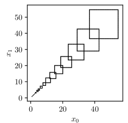
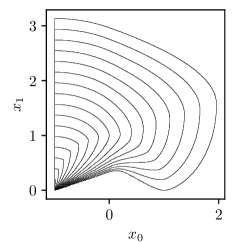
Figure 4 shows the resulting approximate reachable set boundaries generated by Algorithm 4. Sets shown are taken at times $t\in\{\tfrac{j}{16}:0\leq j\leq 16\}.$

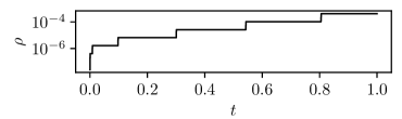
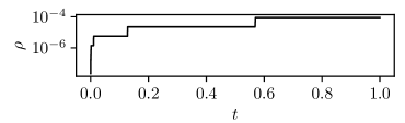
Figure 5 shows that the adaptive refinement strategy of Algorithm 4 works as intended. Initially, the reachable set is small, and a very fine temporal and spatial discretization can be selected at a low cost. Since the local errors are propagated exponentially, choosing a small mesh size near $t=0$ is very desirable. The opposite arguments hold for larger $t$ .

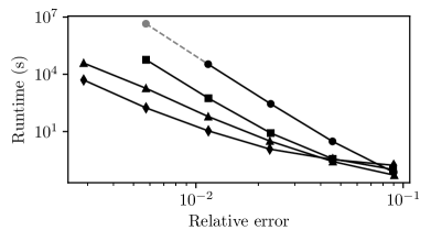
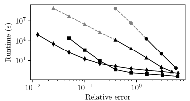
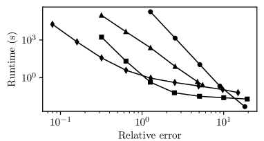
To test the performance of Algorithm 4 (BA) against previous algorithms BU, EA, and EU, we now consider system (70) with $L=1,2,3,4$ . Figure 6 shows that in terms of runtime, Algorithm BA from this paper performs best. Interestingly, the rate at which the runtime increases is very similar for both boundary methods, BA and BU, as well as for both Euler methods EA and EU.

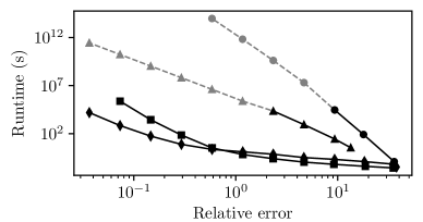
The following example is inspired by [14, Example 4.1].

Example 7.2.

Let $T=1$ , and consider the problem

\dot{x}_{1}\in[0,1]\pi x_{2},\quad\dot{x}_{2}\in-[0,1]\pi x_{1},\quad x(0)=(-1,0)\in\mathbb{R}^{2}

(71)

with Lipschitz constant $L=\pi$ and bound $P=\pi^{2}.$

The approximate reachable set boundaries generated by Algorithm 4 are shown in Figure 7 at times $t\in\{\frac{j}{16}:0\leq j\leq 16\}$ .

Figures 8 and 9 are the equivalent of Figures 5 and 6 for system (71), and show that Algorithm 4 still exhibits the desired behavior when applied to a less straightforward system.

8 Conclusion

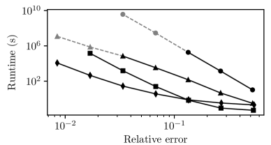
Runge-Kutta methods for computing reachable sets have seen significant advancements over the past decades, as illustrated in Figures 6 and 9. The Euler scheme with uniform discretization from [4, 9] achieved meaningful error bounds only for control systems with very small control sets or over very short time intervals. The boundary tracking algorithm with uniform discretization from [15] reduced the computational cost dramatically, but computations with decent accuracy remained a challenge.

The adaptive Euler scheme from [17] outperforms [15] at low and moderate accuracy, but underperforms it asymptotically, because it tracks full-dimensional sets. Algorithm 4 presented in this paper integrates techniques from both [15] and [17] to overcome this issue. All in all, we see in Figures 6 and 9 that the computational cost for a prescribed precision has been brought down by many orders of magnitude.

While we have proved that Algorithm 4 converges, we have not been able to prove bounds on its performance that reflect its behavior in computational experiments. For now, this remains an open problem. In addition, it would be desirable to develop boundary tracking methods and adaptive refinement techniques based on semi-implicit and fully implicit schemes, which are better suited for stiff systems.

Acknowledgement

This work has partly been supported by an Australian Government Research Training Program (RTP) Scholarship.

References

[1] M. Althoff, O. Stursberg, and M. Buss. Computing reachable sets of hybrid systems using a combination of zonotopes and polytopes. Nonlinear Anal. Hybrid Syst., 4(2):233–249, 2010.
[2] R. Baier, C. Büskens, I.A. Chahma, and M. Gerdts. Approximation of reachable sets by direct solution methods for optimal control problems. Optim. Methods Softw., 22(3):433–452, 2007.
[3] R. Baier, M. Gerdts, and I. Xausa. Approximation of reachable sets using optimal control algorithms. Numer. Algebra Control Optim., 3(3):519–548, 2013.
[4] W.-J. Beyn and J. Rieger. Numerical fixed grid methods for differential inclusions. Computing, 81(1):91–106, 2007.
[5] R.M. Colombo, T. Lorenz, and N. Pogodaev. On the modeling of moving populations through set evolution equations. Discrete Contin. Dyn. Syst., 35(1):73–98, 2015.
[6] M. Gerdts and I. Xausa. Avoidance trajectories using reachable sets and parametric sensitivity analysis. In System modeling and optimization, volume 391 of IFIP Adv. Inf. Commun. Technol., pages 491–500. Springer, Heidelberg, 2013.
[7] A. Girard, C. Le Guernic, and O. Maler. Efficient computation of reachable sets of linear time-invariant systems with inputs. In Hybrid systems: computation and control, volume 3927 of Lecture Notes in Comput. Sci., pages 257–271. Springer, Berlin, 2006.
[8] R. Klette and A. Rosenfeld. Digital geometry. Morgan Kaufmann Publishers, San Francisco, CA; Elsevier Science B.V., Amsterdam, 2004. Geometric methods for digital picture analysis.
[9] V.A. Komarov and K.È. Pevchikh. A method for the approximation of attainability sets of differential inclusions with given accuracy. Zh. Vychisl. Mat. i Mat. Fiz., 31(1):153–157, 1991.
[10] A.B. Kurzhanski and P Varaiya. Ellipsoidal techniques for reachability analysis. In Hybrid Systems: Computation and Control, pages 202–214, Berlin, Heidelberg, 2000. Springer Berlin Heidelberg.
[11] C. Le Guernic and A. Girard. Reachability analysis of linear systems using support functions. Nonlinear Analysis: Hybrid Systems, 4(2):250–262, 2010. IFAC World Congress 2008.
[12] J.R. Munkres. Topology. Prentice Hall, Inc., Upper Saddle River, NJ, second edition, 2000.
[13] F. Parise, M.E. Valcher, and J. Lygeros. Computing the projected reachable set of stochastic biochemical reaction networks modeled by switched affine systems. IEEE Trans. Automat. Control, 63(11):3719–3734, 2018.
[14] W. Riedl, R. Baier, and M. Gerdts. Optimization-based subdivision algorithm for reachable sets. J. Comput. Dyn., 8(1):99–130, 2021.
[15] J. Rieger. Robust boundary tracking for reachable sets of nonlinear differential inclusions. Found. Comput. Math., 15(5):1129–1150, 2015.
[16] J. Rieger and K. Wawryk. Restriction and interpolation operators for digital images and their boundaries. arXiv, 2024, arXiv:2407.18511.
[17] J. Rieger and K. Wawryk. Towards optimal space-time discretization for reachable sets of nonlinear control systems. J. Comput. Dyn., 11(2):153–173, 2024.
[18] M. Rungger and M. Zamani. Accurate reachability analysis of uncertain nonlinear systems. In Proceedings of the 21st international conference on hybrid systems: Computation and control (part of CPS week), pages 61–70, 2018.
[19] M. Serry and G. Reissig. Overapproximating reachable tubes of linear time-varying systems. IEEE Trans. Automat. Control, 67(1):443–450, 2022.
[20] V. Veliov. Second order discrete approximations to strongly convex differential inclusions. Systems Control Lett., 13(3):263–269, 1989.
[21] V. Veliov. On the time-discretization of control systems. SIAM J. Control Optim., 35(5), 1997.