1-1-1 Noji-higashi, Kusatsu, 525-8577, Japan22affiliationtext: Graduate School of Engineering Science, Osaka University
1-3, Machikaneyama, Toyonaka, Osaka, 560-8531, Japan
Eigenvalue analysis of three-state quantum walks
with general coin matrices
Abstract
Mathematical analysis on the existence of eigenvalues is vital, as it corresponds to the occurrence of localization, an exceptionally important property of quantum walks. Previous studies have demonstrated that eigenvalue analysis utilizing the transfer matrix proves beneficial for space inhomogeneous three-state quantum walks with a specific class of coin matrices, including Grover matrices. In this research, we turn our attention to the transfer matrix of three-state quantum walks with a general coin matrix. Building upon previous research methodologies, we dive deeper into investigating the properties of the transfer matrix and employ numerical analysis to derive eigenvalues for models that were previously unanalyzable.
1 Introduction
Quantum walks (QWs) are fundamental models for understanding quantum dynamics. Despite their apparent simplicity, quantum walks exhibit a wide range of intricate quantum features, making them essential tools in various domains, including the study of topological phases [1] and the formulation of models and designs for quantum algorithms [2, 3, 4]. Within the context of QWs, the combination of the coin operator and the shift operator determines how the system evolves. A vital part of studying QWs is looking at the spectral properties of the time evolution operator. This helps us understand the behaviors and features of the walk, thereby enriching our comprehension of the underlying dynamics.
In this paper, our focus is on three-state QWs on a one-dimensional integer lattice, which involves working within an infinite-dimensional Hilbert space. This model is intensively studied in various articles with different contexts [5, 6, 7, 8, 9, 10, 11, 12, 13, 14, 15, 16, 17, 18, 19, 20]. It is well-known that the occurrence of localization, a characteristic property of QWs, is equivalent to the existence of eigenvalues of the time evolution operator. Moreover, a quantitative investigation of localization can be conducted by deriving the time-averaged limit distribution using the eigenvalues and eigenvectors [21]. The transfer matrix method stands as a powerful tool for eigenvalue analysis and has been applied to several types of QW models [22, 23, 24], and even for non-unitary QWs [25]. We specifically consider the two-phase model with a finite number of defects. Previous studies [24] have conducted eigenvalue analysis for three-state QWs with a specific class of coin matrices, including Grover matrices, through the transfer matrix method. In contrast, this work extends the result by demonstrating that the method remains applicable and effective even for cases involving a general coin matrix.
Calculating explicit eigenvalues analytically for a general coin matrix remains highly challenging. Therefore, we resort to numerical calculations to determine eigenvalues, utilizing the method of the transfer matrix. For our numerical analysis, we concentrate on one-defect and two-phase Fourier walks. The Fourier walk has been intensively studied by [26, 27, 28] for the space-homogeneous model, where the coin matrices are identical at any position. Notably, it has been proven that the Fourier walk does not exhibit localization for the homogeneous model. However, we numerically demonstrate that the Fourier walk does exhibit localization for both the one-defect and two-phase models.
The remainder of this paper is organized as follows. In Section 2, we define our three-state QWs with a self-loop on the integer lattice. Section 3 introduces the transfer matrix with a general coin matrix and establishes methods for the eigenvalue problem. Theorem 1 constitutes the main theorem, providing a necessary and sufficient condition for the eigenvalue problem. Section 4 is dedicated to the numerical analysis of the Fourier walk. We present figures to visually depict the results of the numerical analysis on the eigenvalue equation and its probability distribution, thereby illustrating the occurrence of localization and the existence of the eigenvalue.
2 Definition
We define a three-state QW on the integer lattice . Let us define the Hilbert space as
Here, denotes the set of complex numbers. The quantum state is expressed as
Let be a sequence of unitary matrices, which is written as below:
Here, we assume that . The coin operator is then defined using the coin matrices as:
Next, we define a shift operator that moves to the left and to the right.
Finally, the time evolution of the QW is determined by the following unitary operator
We impose a condition essential for considering eigenvalue analysis with our method.
where . We say the model with this condition as two-phase QW with finite number of defects. As a remark, we can easily replace with periodic coin matrices by following the previous research [29]. However we opt not to explore this generalization as it leads to notably more complex notation. For an initial state , the finding probability of a walker in position at time is defined by
where is the set of non-negative integers. We say that the exhibits localization if there exists a position and an initial state satisfying . It is known that the QW exhibits localization if and only if there exists an eigenvalue of , that is, there exists and such that
Let hereafter denote the set of eigenvalues of .
3 Eigenvalue analysis with transfer matrix
The eigenvalue equation can be rewritten as the following system of equations:
| (1) | |||
| (2) | |||
| (3) |
where
Here, we define transfer matrices by
then equations (1), (2) can be expressed as
From the unitarity of the coin matrix, we can write
where and denote the submatrix obtained by excluding the -th row and -th column of . Using the above expression, we can simplify each component of the transfer matrix as:
and we can further calculate
Hence, we can simplify the expression of the transfer matrix as
Note that, when , we cannot construct a transfer matrix. Therefore, we must treat this case separately. Let us define
and we consider the case first. For simplification, we may write as henceforward. Let and , we define as follows:
| (4) |
where and . Let be a set of generalized eigenvectors and be a set of reduced vectors defined by (4):
For , we define a bijective map by
Here, the inverse of is given as
for . Thus, from the definition, if and only if there exists such that . We can also see that is equivalent to .
Corollary 3.1.
Let satisfying for all is the eigenvalue of , i.e., , if and only if there exists such that , and the associated eigenvector of becomes .
The subsequent property is pivotal in formulating the method for the eigenvalue problem.
Proposition 3.2.
For all and , we have
Proof.
By direct calculation, we have
Therefore,
which implies
∎
Thus, we can convince that the following two eigenvalues , of the transfer matrix satisfies
In this paper, we define the square root of the complex number as . Consequently, we designate as one of such that , and such that Additionally, we introduce and as normalized eigenvector of corresponding to and , respectively.
Proposition 3.3.
The condition holds if and only if:
Proof.
We aim to determine the conditions for
This is equivalent to
| (5) |
For this to hold, it is necessary that
Here, denotes “if and only if”. By using (5), we deduce
Squaring both side, we obtain the equivalent statement:
| (6) | ||||
| (7) |
It can also be verified that if (7) holds, so does (5). This completes the proof. ∎
Let
With this, we present the following theorem:
Theorem 1.
is the eigenvalue of , i.e., , if and only if the following two conditions are satisfied:
Proof.
We know from Corollary 3.1 that if and only if there exists such that . If , both and become 1 by definition. Since is given as (4), for all . Therefore, is a necessary condition for . Next we assume that , then and hold. Since is expressed by and transfer matrices, there exists such that if and only if there exists such that , that is, The conclusions drawn from the above discussions validate the statement. ∎
Corollary 3.4.
is the eigenvalue of , i.e., , if and only if the following conditions are met:
From Theorem 1, for , the eigenvector is given by , where becomes
with Furthermore, it is straightforward to verify that .
If for some , we cannot construct a transfer matrix at . Therefore, we have to deal with this case separately.
Lemma 3.5.
For all , we have
Proof.
We assume that , which means
Then, we can easily calculate that
Similarly implies
and .
∎
Proposition 3.6.
Consider . The equation is satisfied if and only if:
for with and
| (8) |
for with .
Proof.
Assume By our previous lemma, this implies Given this, we have and
where
This is equivalent to
∎
As a consequence of the last proposition, we obtain the following prposition.
Proposition 3.7.
is eigenvalue of if and only if
We get the following corollary, which was also proved in [30].
4 Numerical analysis on Fourier walk
In this section, we deal with the Fourier walk studied in [26, 27, 28]. Let us consider the following Fourier matrix as a coin matrix.
where .
4.1 One-defect model
Consider the coin matrix defined as:
with some .
Proposition 4.1.
For a one-defect Fourier walk,
Proof.
From Proposition 3.7, we know that is not an eigenvalue of since
Also, we prove that is not an eigenvalue of by contradiction. Assuming that then
| (9) |
and
must be satisfied. However, by direct calculation, we obtain the contradiction. ∎
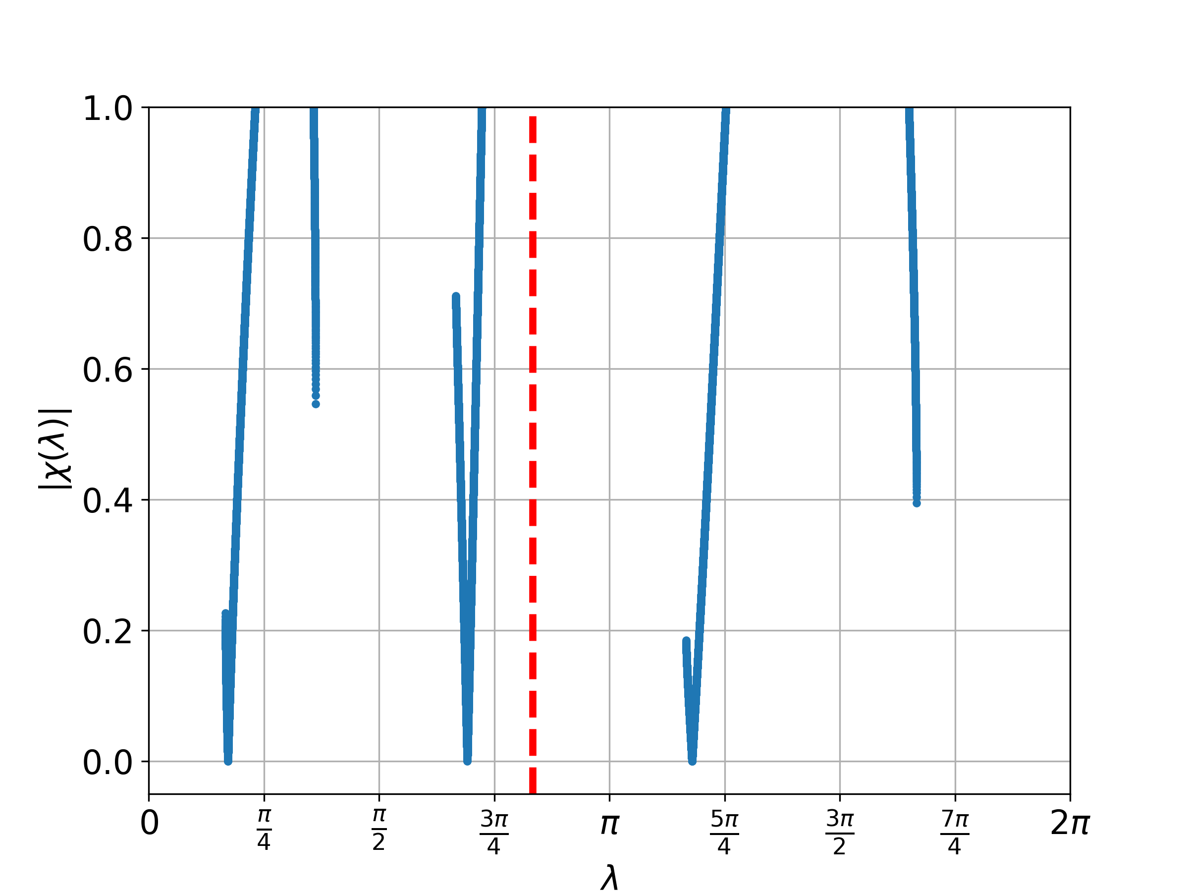
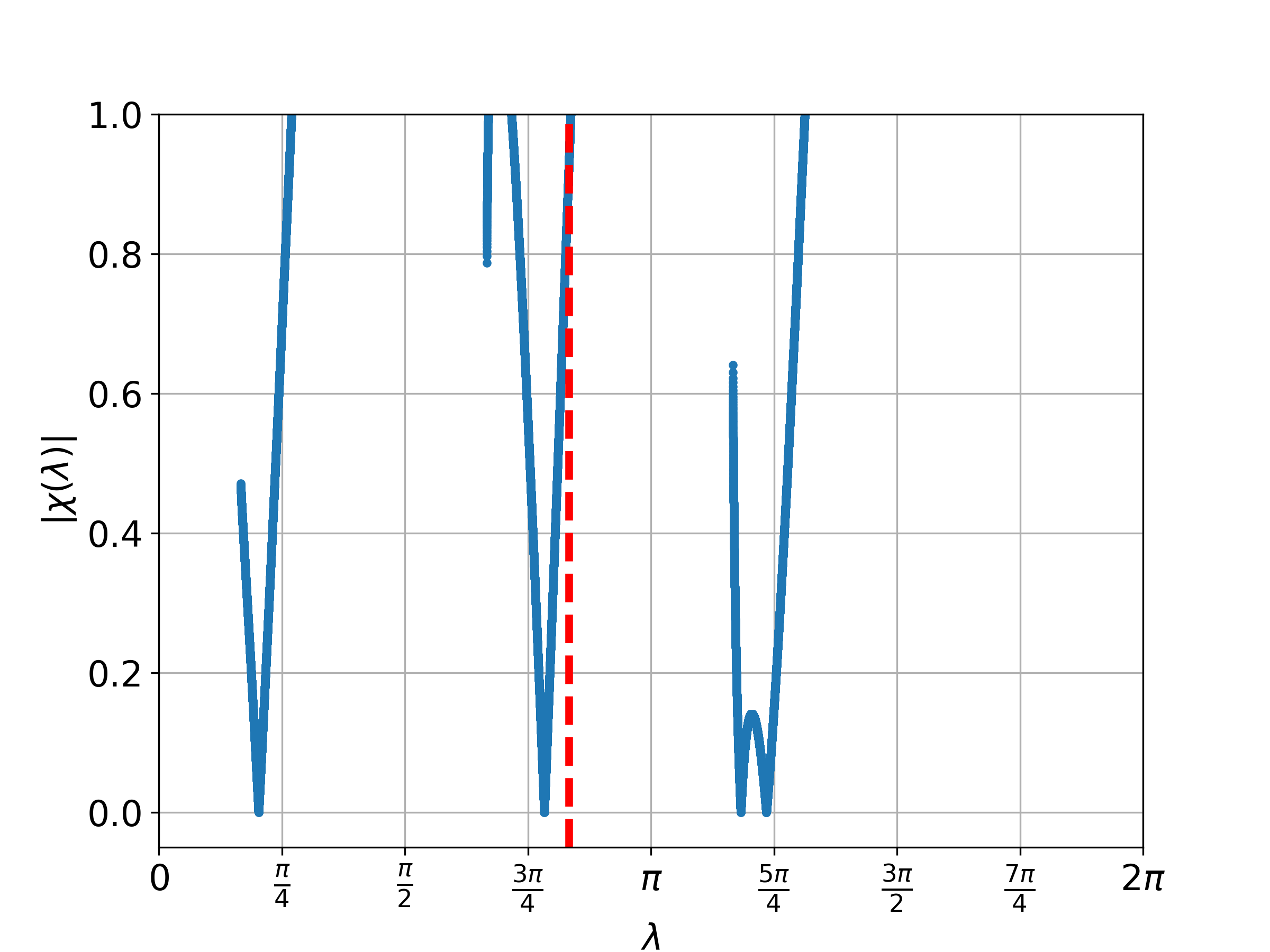
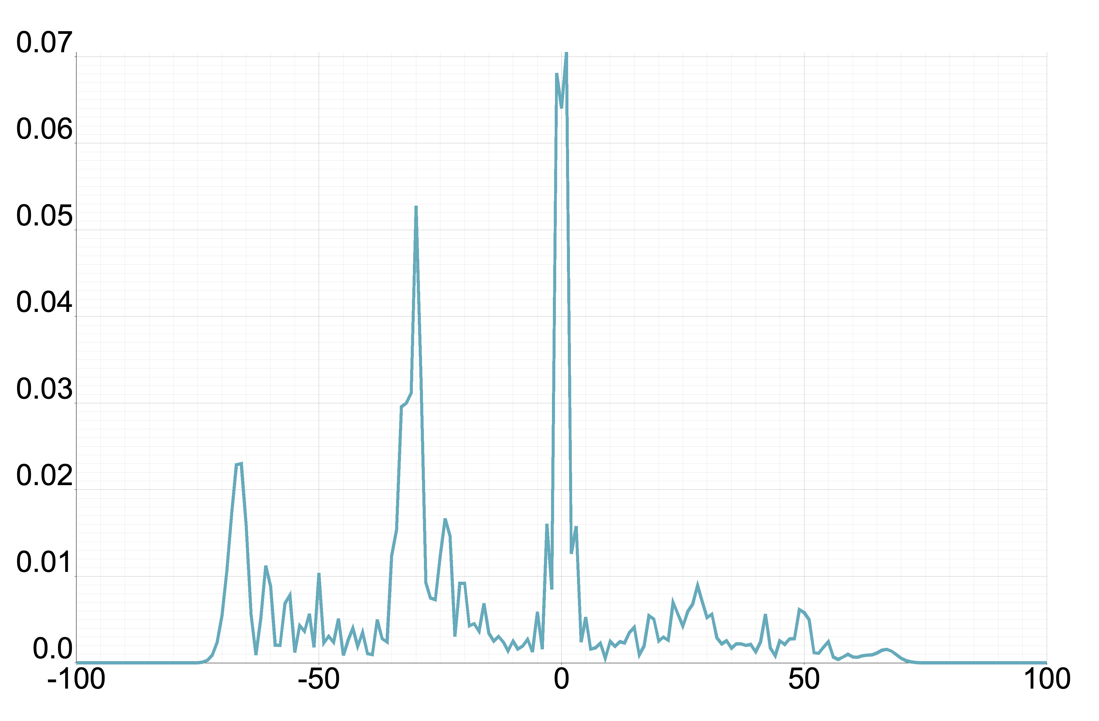
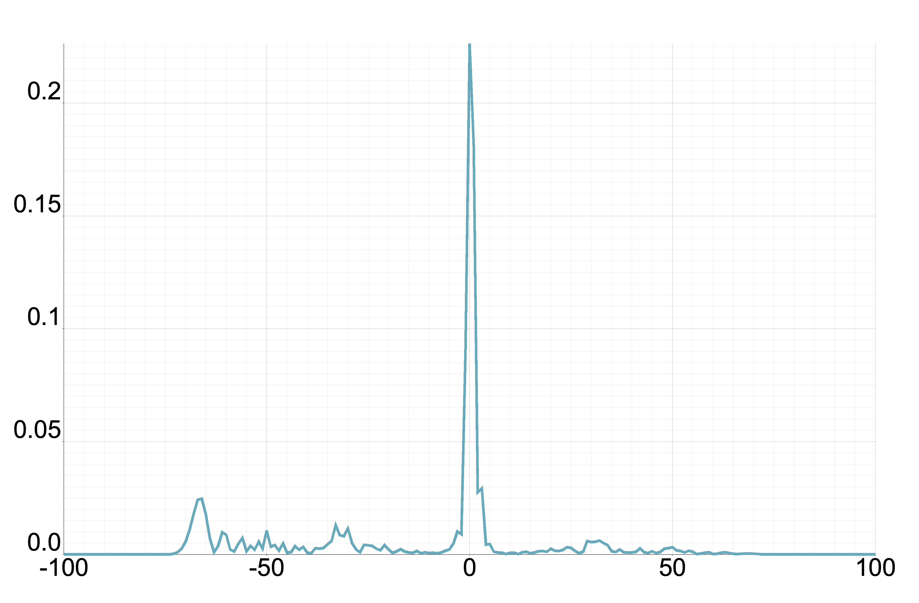
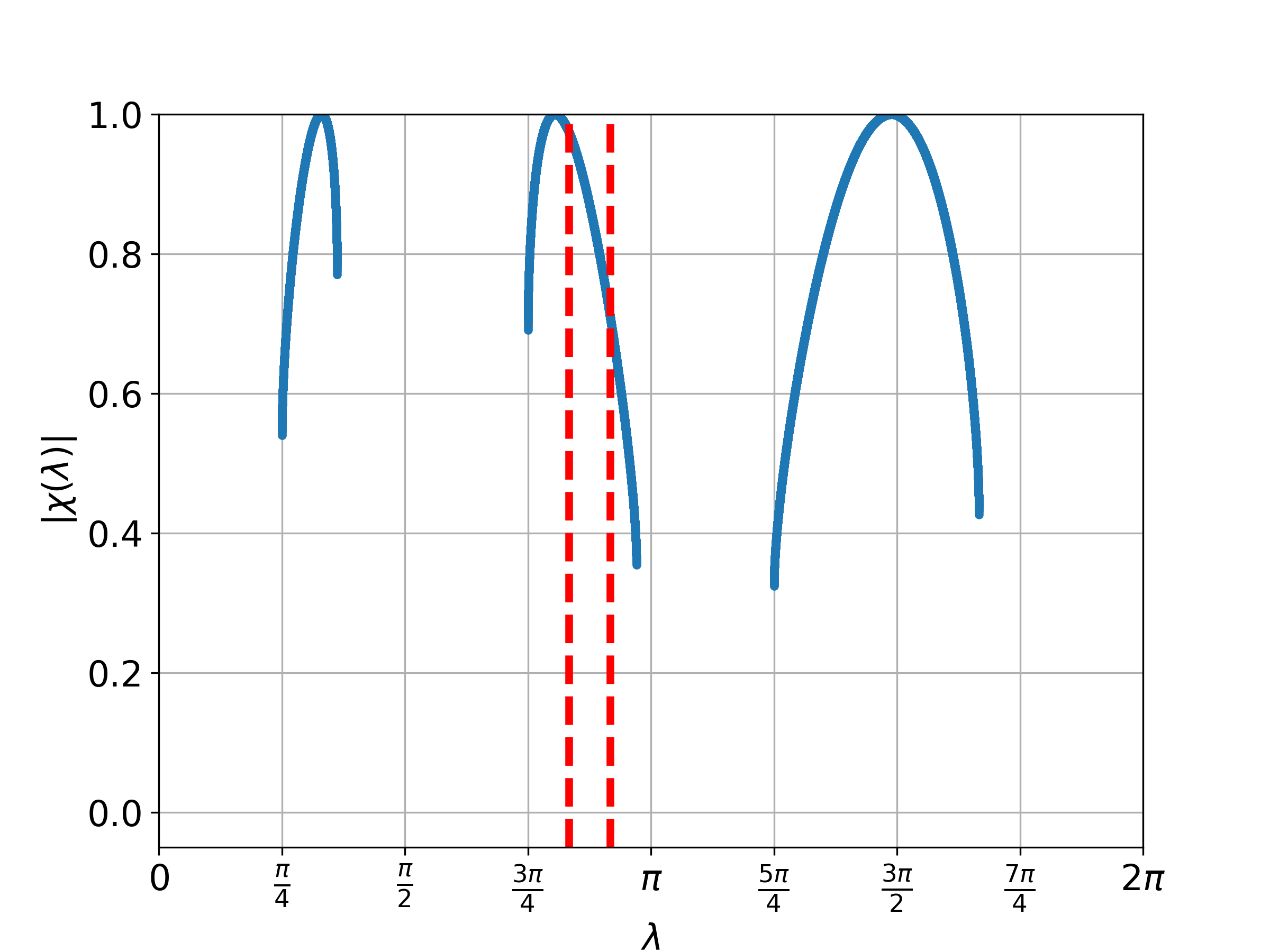
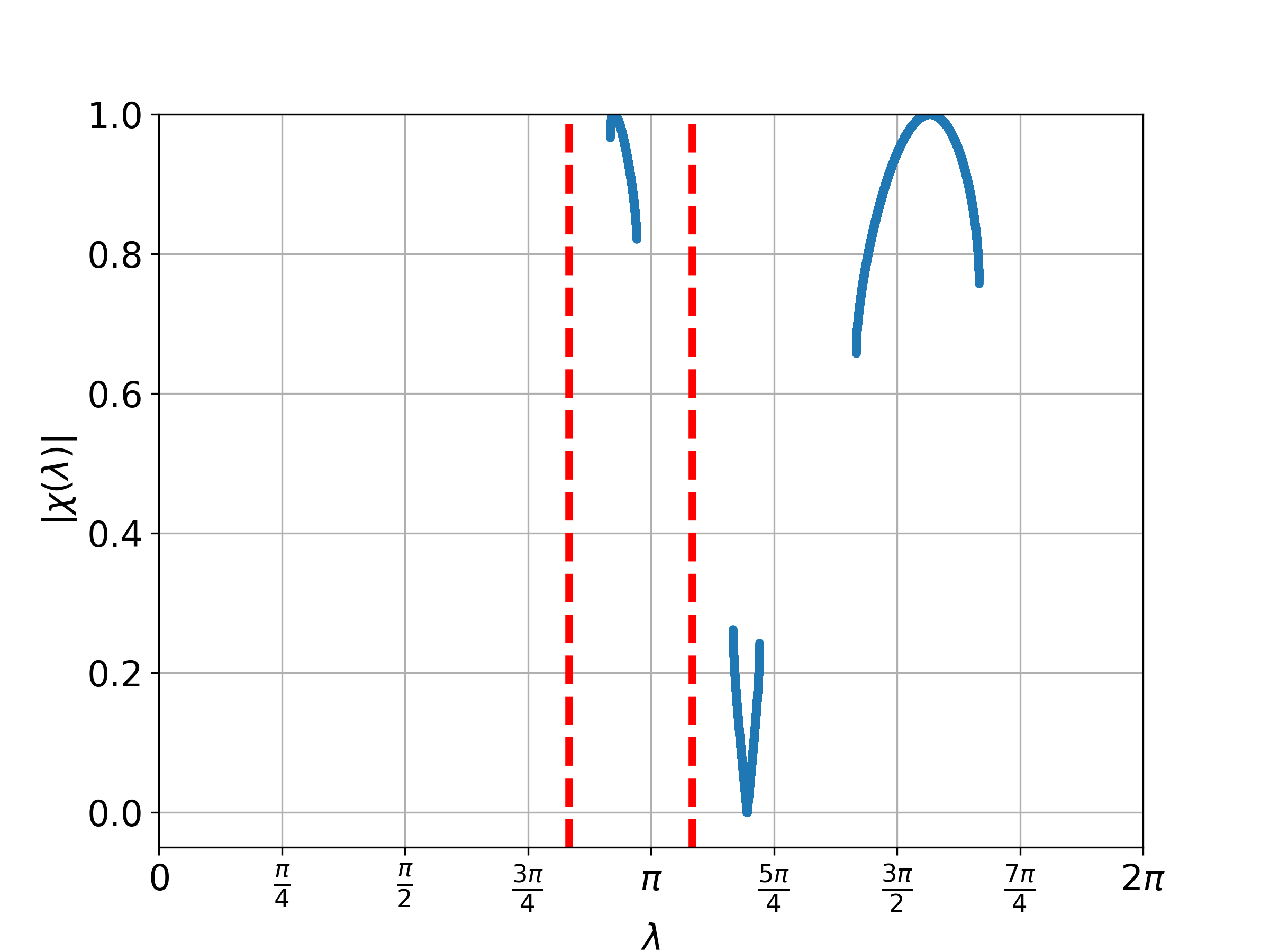
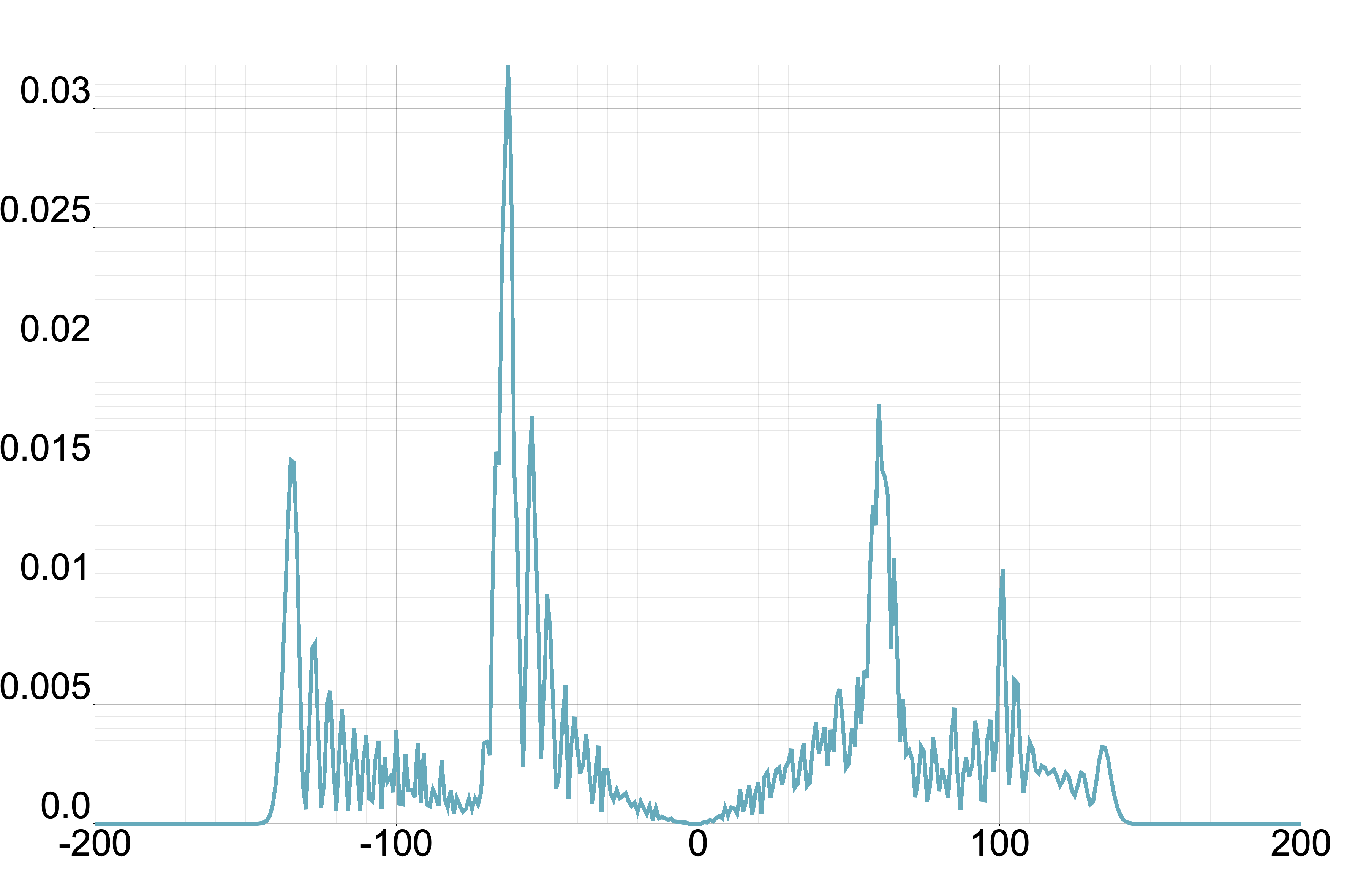
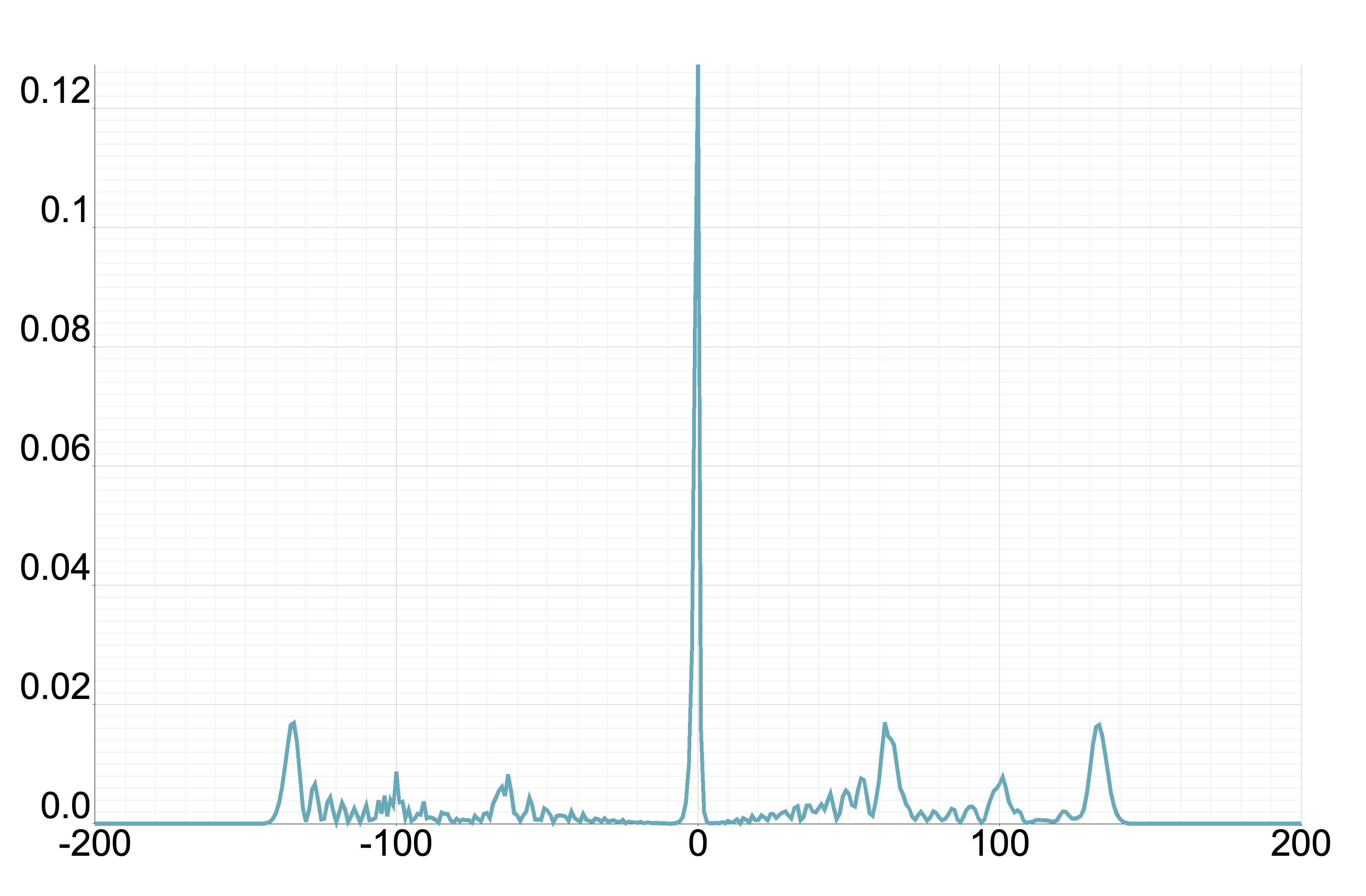
From this proposition, we understand that we only need to consider . Figure 1 displays the plot of for different values of where . Meanwhile, Figure 2 illustrates the probability distribution corresponding to Figure 1 for the one-defect Fourier walk.
4.2 Two-phase model
Consider the coin matrix defined as:
with some . The following proposition can be proved similarly to Proposition 4.1.
Proposition 4.2.
For a two-phase Fourier walk,
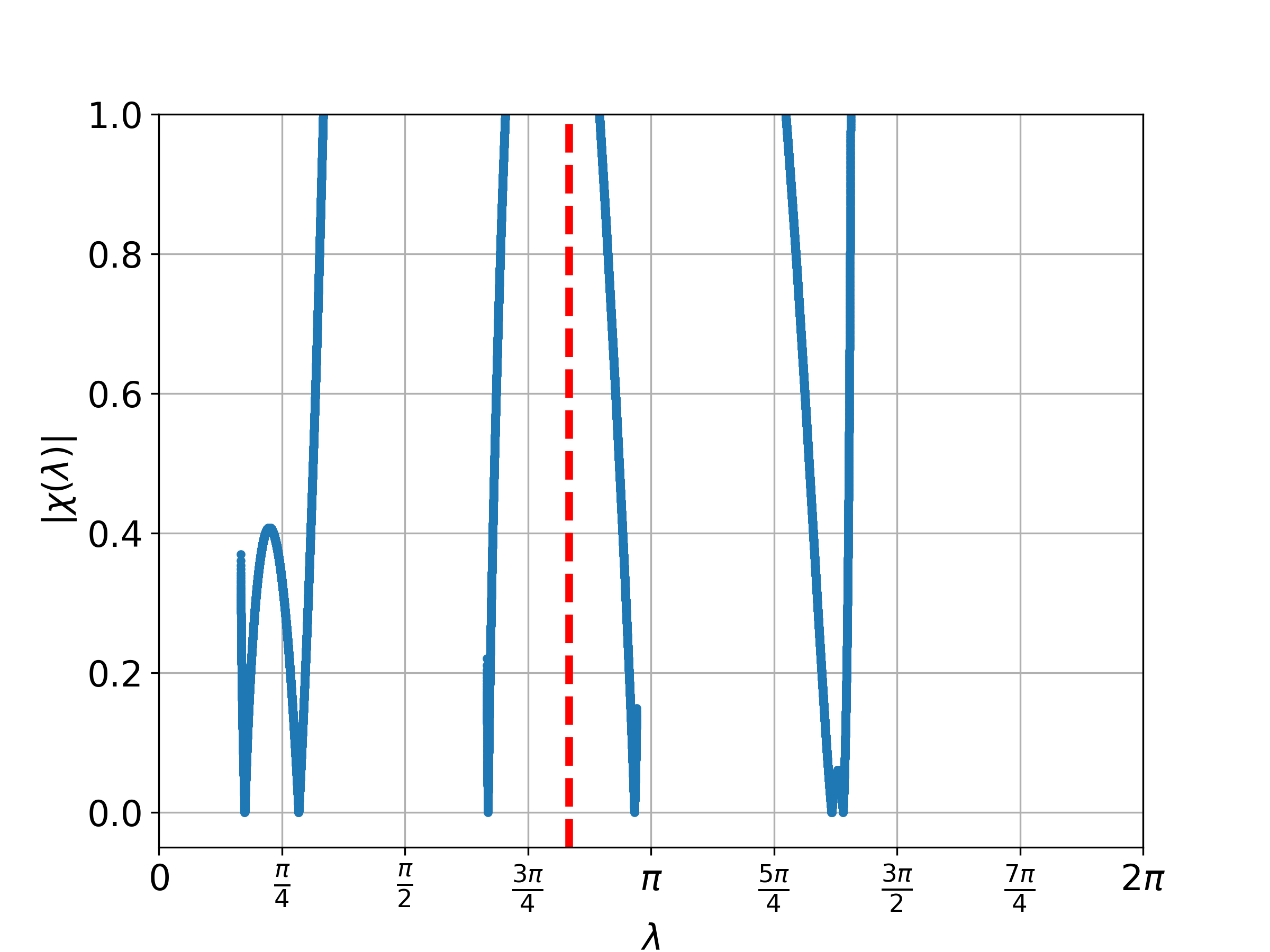
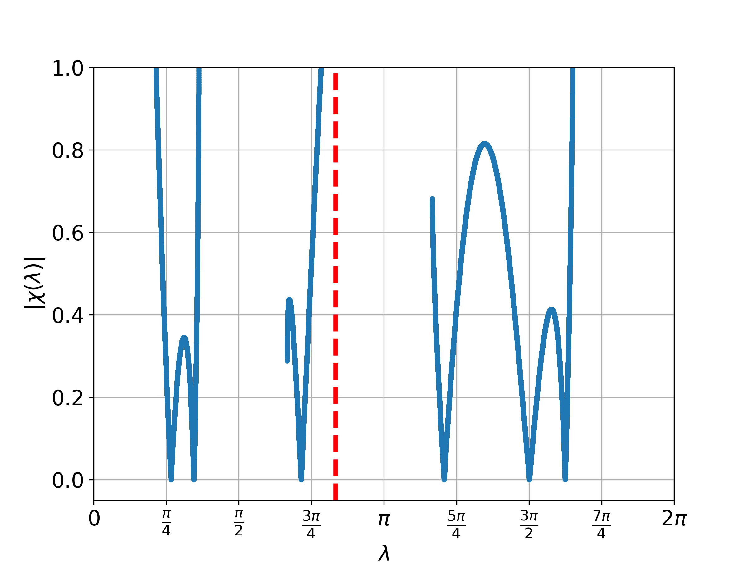
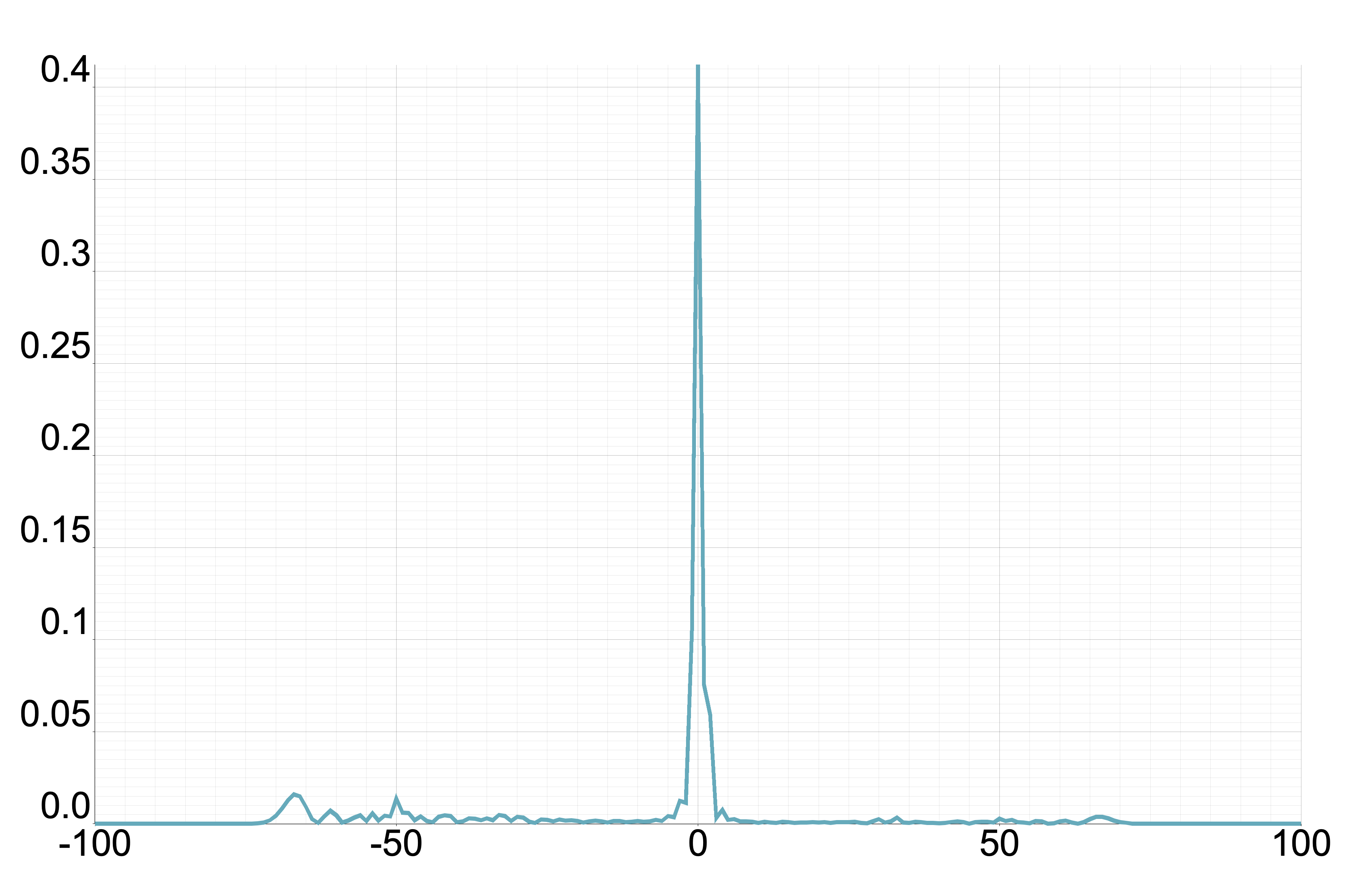
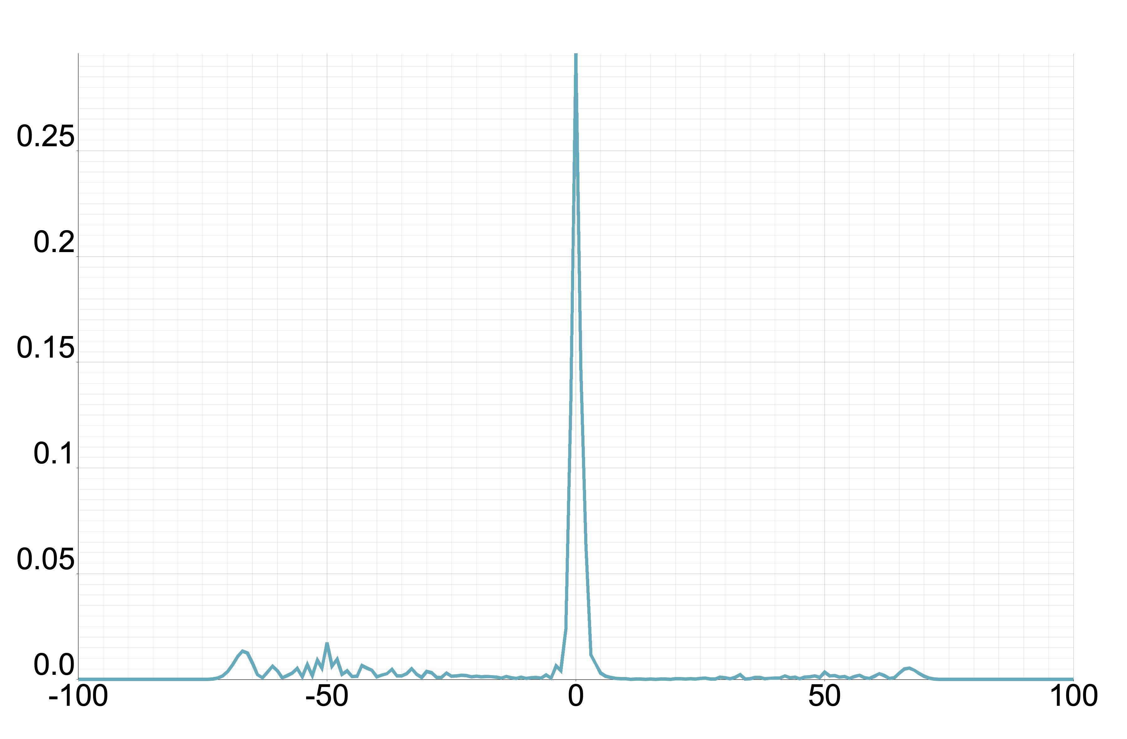
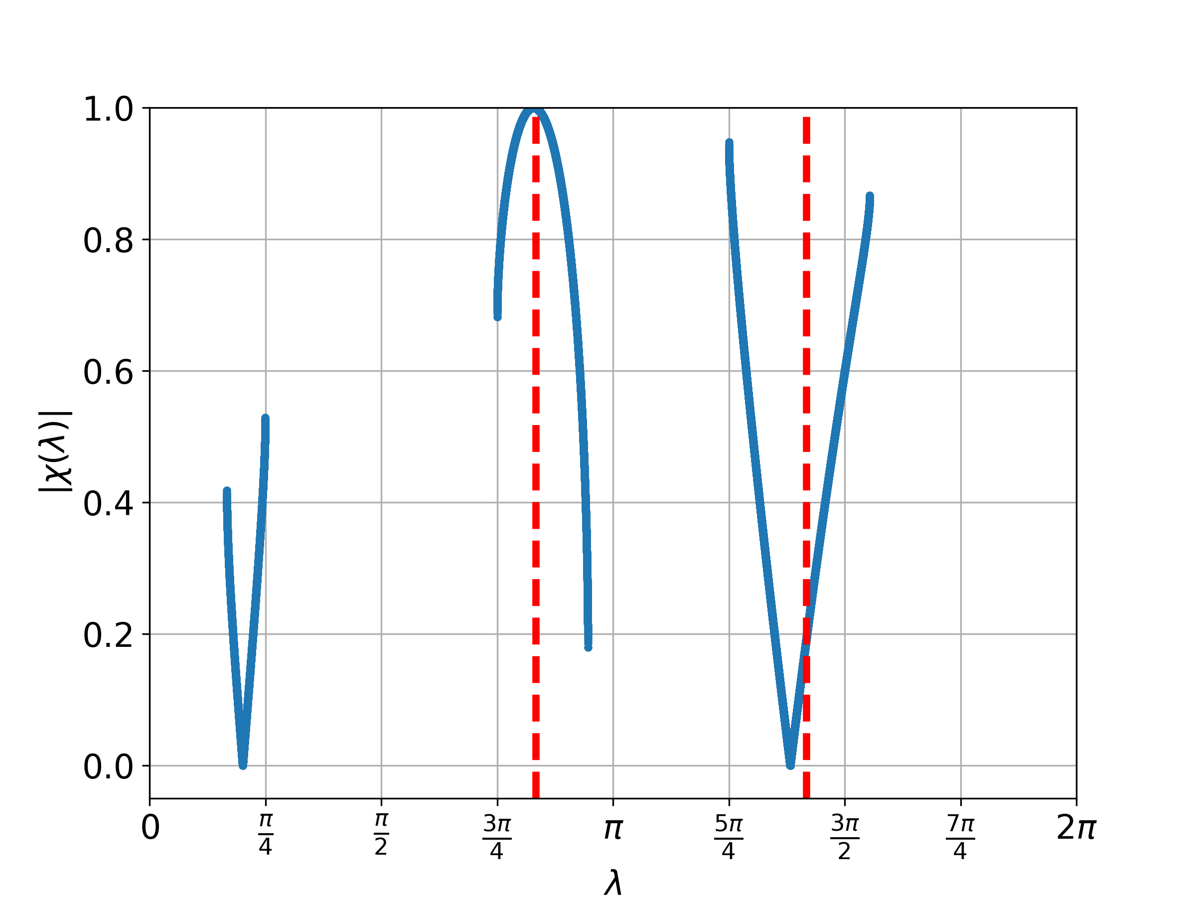
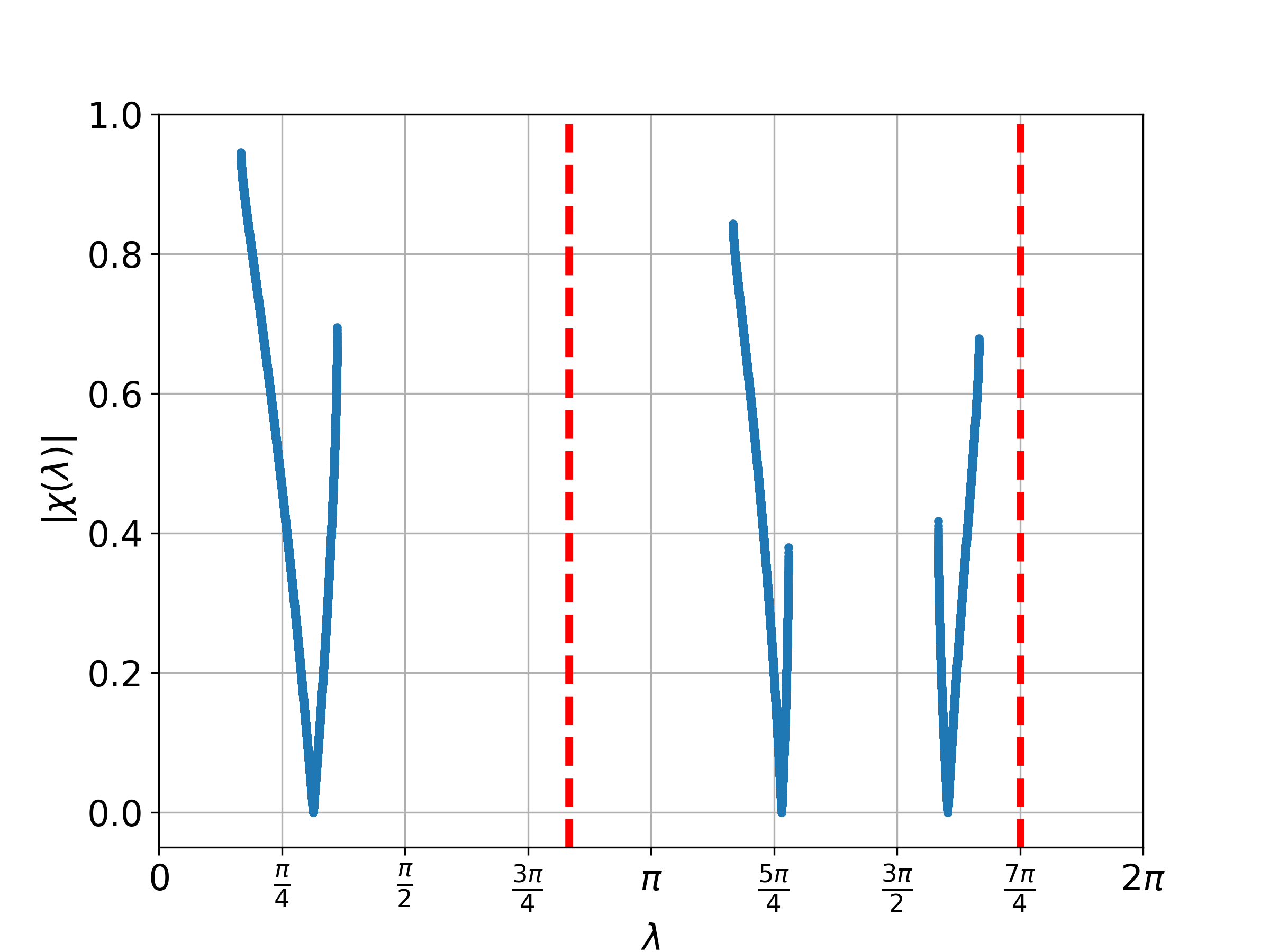
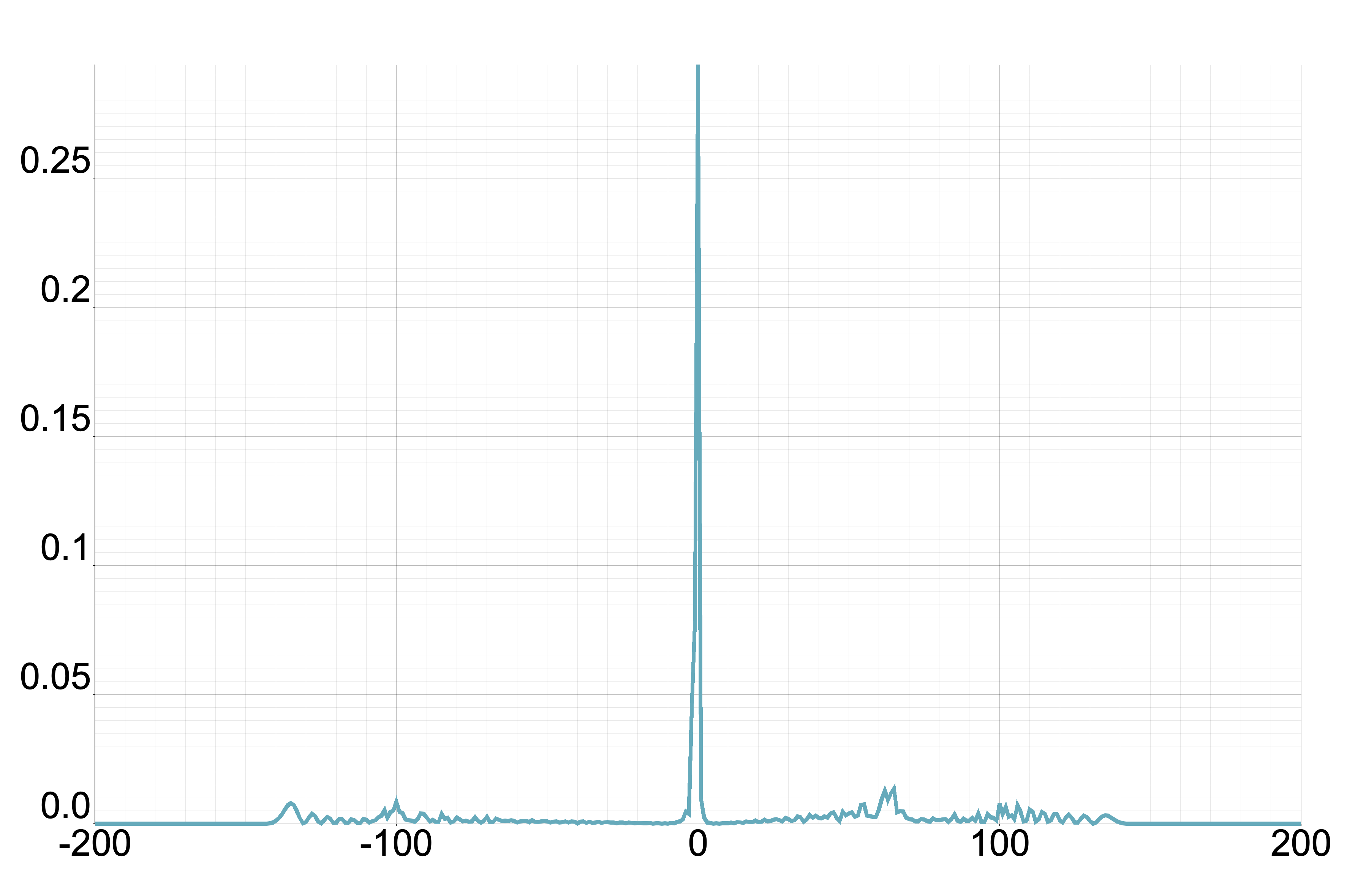
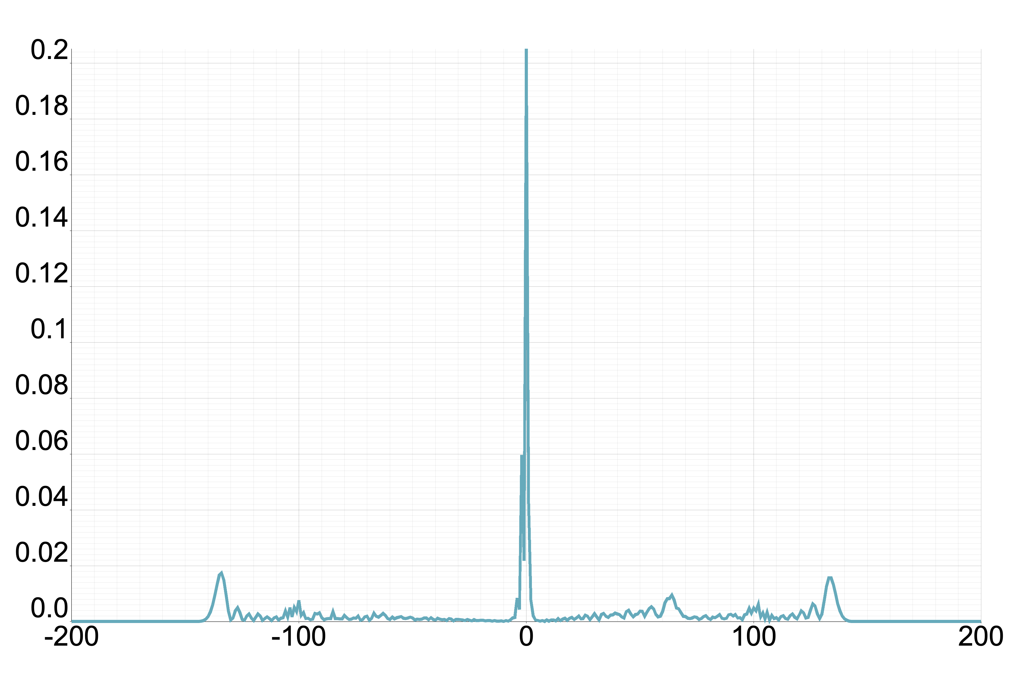
From this proposition, we understand that we only have to consider . Figure 3 displays the plot of for different values of where . Meanwhile, Figure 4 illustrates the probability distribution corresponding to Figure 3 for the two-phase Fourier walk.
Acknowledgment
The author C. Kiumi was supported by JSPS KAKENHI Grant Number JP22KJ1408.
References
- [1] T. Kitagawa, M. S. Rudner, E. Berg, E. Demler, Exploring topological phases with quantum walks, Phys. Rev. A 82 (3) (2010) 033429.
- [2] S. Apers, A. Scarlet, Quantum fast-forwarding: Markov chains and graph property testing, Quantum Inf. Comput. 19 (3&4) (2019) 181–213.
- [3] A. Gilyén, Y. Su, G. H. Low, N. Wiebe, Quantum singular value transformation and beyond: exponential improvements for quantum matrix arithmetics, in: Proceedings of the 51st Annual ACM SIGACT Symposium on Theory of Computing, ACM, 2019.
- [4] S. Apers, A. Gilyén, S. Jeffery, A unified framework of quantum walk search, in: 38th International Symposium on Theoretical Aspects of Computer Science (STACS 2021), Vol. 187 of Leibniz International Proceedings in Informatics (LIPIcs), Schloss Dagstuhl – Leibniz-Zentrum für Informatik, 2021, pp. 6:1–6:13.
- [5] N. Inui, N. Konno, Localization of multi-state quantum walk in one dimension, Phys. A: Stat. Mech. Appl. 353 (2005) 133–144.
- [6] N. Inui, N. Konno, E. Segawa, One-dimensional three-state quantum walk, Phys. Rev. E Stat. Nonlin. Soft Matter Phys. 72 (5 Pt 2) (2005) 056112.
- [7] S. Falkner, S. Boettcher, Weak limit of the three-state quantum walk on the line, Phys. Rev. A 90 (1) (2014) 012307.
- [8] M. Štefaňák, I. Bezděková, I. Jex, Limit distributions of three-state quantum walks: The role of coin eigenstates, Phys. Rev. A 90 (1) (2014) 012342.
- [9] D. Li, M. Mc Gettrick, W. Zhang, K. Zhang, One-dimensional lazy quantum walks and occupancy rate, Chin. Phys. B 24 (5) (2015) 050305.
- [10] T. Machida, Limit theorems of a 3-state quantum walk and its application for discrete uniform measures, Quantum Inf. Comput. (2015) 406–418.
- [11] C. Wang, W. Wang, d. X. Lu, Limit theorem for a Time-Inhomogeneous Three-State quantum walk on the line, J. Comput. Theor. Nanosci. 12 (12) (2015) 5164–5170.
- [12] Y.-Z. Xu, G.-D. Guo, S. Lin, One-Dimensional Three-State quantum walk with Single-Point phase defects, Int. J. Theor. Phys. 55 (9) (2016) 4060–4074.
- [13] H. Kawai, T. Komatsu, N. Konno, Stationary measures of three-state quantum walks on the one-dimensional lattice, Yokohama Math. J. 63 (2017) 59–74.
- [14] J. Rajendran, C. Benjamin, Playing a true parrondo’s game with a three-state coin on a quantum walk, EPL 122 (4) (2018) 40004.
- [15] T. Endo, T. Komatsu, N. Konno, T. Terada, Stationary measure for three-state quantum walk, Quantum Inf. Comput. 19 (11&12) (2019) 901–912.
- [16] A. Saha, S. B. Mandal, D. Saha, A. Chakrabarti, One-Dimensional lazy quantum walk in ternary system, IEEE Trans. Quant. Eng. 2 (2021) 1–12.
- [17] C. Wang, X. Lu, W. Wang, The stationary measure of a space-inhomogeneous three-state quantum walk on the line, Quantum Inf. Process. 14 (3) (2015) 867–880.
- [18] P. R. N. Falcão, A. R. C. Buarque, W. S. Dias, G. M. A. Almeida, M. L. Lyra, Universal dynamical scaling laws in three-state quantum walks, Phys. Rev. E 104 (2021) 054106.
- [19] C. Kiumi, A new type of quantum walks based on decomposing quantum states, Quantum Inf. Comput. 21 (7&8) (2021) 541–556.
- [20] T. Yamagami, E. Segawa, T. Mihana, A. Röhm, R. Horisaki, M. Naruse, Bandit algorithm driven by a classical random walk and a quantum walk, Entropy 25 (6) (2023).
- [21] C. Kiumi, K. Saito, Strongly trapped space-inhomogeneous quantum walks in one dimension, Quantum Inf. Process. 21 (9) (2022).
- [22] S. Endo, T. Endo, T. Komatsu, N. Konno, Eigenvalues of Two-State quantum walks induced by the hadamard walk, Entropy 22 (1) (2020).
- [23] C. Kiumi, K. Saito, Eigenvalues of two-phase quantum walks with one defect in one dimension, Quantum Inf. Process. 20 (5) (2021).
- [24] C. Kiumi, Localization of space-inhomogeneous three-state quantum walks, J. Phys. A: Math 55 (22) (2022) 225205.
- [25] C. Kiumi, K. Saito, Spectral analysis of non-unitary two-phase quantum walks in one dimension (2022). arXiv:2205.11046.
- [26] K. Saito, Periodicity for the fourier quantum walk on regular graphs, Quantum Inf. and Comput. 19 (1&2) (2019) 23–34.
- [27] M. Asano, T. Komatsu, N. Konno, A. Narimatsu, The fourier and grover walks on the two-dimensional lattice and torus, Yokohama Math. J. 65 (2019) 13–32.
- [28] A. Narimatsu, Localization does not occur for the fourier walk on the multi-dimensional lattice, Quantum Inf. Comput. 21 (5&6) (2021) 387–394.
- [29] C. Kiumi, Localization in quantum walks with periodically arranged coin matrices, Int. J. Quantum Inf. 20 (05) (2022).
- [30] C. K. Ko, E. Segawa, H. J. Yoo, One-dimensional three-state quantum walks: Weak limits and localization, Infin. Dimens. Anal. Quantum Probab. Relat. Top. 19 (04) (2016) 1650025.