Eigenvalue Asymptotics near a flat band in presence of a slowly decaying potential

We denote by $\mathcal{X}=(\mathcal{V},\mathcal{A})$ the standard graph structure in $\mathbb{Z}^{n}$. That is, the set of vertices $\mathcal{V}$ consists of points $\mu\in\mathbb{Z}^{n}$ and the set of oriented edges $\mathcal{A}$ is composed of pairs $(\mu,\nu)$ such that $\nu=\mu\pm\delta_{j}$, where $\{\delta_{j}\}_{j=1}^{n}$ denotes the canonical basis of $\mathbb{Z}^{n}$. An edge in $\mathcal{A}$ is written $\mathrm{e}=(\mu,\nu)$ and its transpose $\overline{\mathrm{e}}:=(\nu,\mu)$. Let us consider the vector spaces of $0-$cochains $C^{0}(\mathcal{X})$ and $1-$cochains $C^{1}(\mathcal{X})$ given by

$$C^{0}(\mathcal{X}):=\{f:\mathcal{V}\to\mathbb{C}\}\text{ ; }\qquad C^{1}(\mathcal{X}):=\{g:\mathcal{A}\to\mathbb{C}\mid g(\mathrm{e})=-g(\overline{\mathrm{e}})\}.$$

The Hilbert spaces $\ell^{2}(\mathcal{V})$ and $\ell^{2}(\mathcal{A})$ are naturally defined by the inner products of cochains: $\langle f_{1},f_{2}\rangle_{0}=\sum_{\mu\in\mathcal{V}}f_{1}(\mu)\overline{f_{2}(\mu)}$ and $\langle g_{1},g_{2}\rangle_{1}=\frac{1}{2}\sum_{e\in\mathcal{A}}g_{1}(e)\overline{g_{2}(e)}$, respectively.

The coboundary operator $d:\ell^{2}(\mathcal{V})\to\ell^{2}(\mathcal{A})$ is defined by

(3)

$$df(\mathrm{e}):=f(\nu)-f(\mu),\quad\text{ for }\mathrm{e}=(\mu,\nu)\in\mathcal{A}\ .$$

This is the discrete version of the exterior derivative and its adjoint $d^{*}:\ell^{2}(\mathcal{A})\to\ell^{2}(\mathcal{V})$ is given at each edge by the finite sum

(4)

$$d^{*}g(\mu)=\sum_{j=1}^{n}g(\mu,\mu\pm\delta_{j}),\quad\text{ for }\mu\in\mathcal{V}.$$

Let us define the Hilbert space $\ell^{2}(\mathcal{X})=\ell^{2}(\mathcal{V})\oplus\ell^{2}(\mathcal{A})$ and denote by $P_{\mathcal{V}}$ and $P_{\mathcal{A}}$ the corresponding projections. Further, we introduce the involution $\tau$ on $\ell^{2}(\mathcal{X})$ by

$$\tau(f,g)=(f,-g)\ .$$

Then, for a strictly positive constant $m$ let us consider the free Dirac operator

$$H_{0}=d+d^{*}+m\tau=\begin{pmatrix}0&d^{*}\\ d&0\end{pmatrix}+m\begin{pmatrix}1&0\\ 0&-1\end{pmatrix}=\begin{pmatrix}m&d^{*}\\ d&-m\end{pmatrix}$$

where we have slightly abused notation by considering $d$ and $d^{*}$ acting on $\ell^{2}(\mathcal{X})$. Note that $H_{0}$ is a Dirac-type operator in the sense that

$$H_{0}^{2}=\begin{pmatrix}\Delta_{0}+m^{2}&0\\ 0&\Delta_{1}+m^{2}\end{pmatrix}$$

where $\Delta_{0}$ is the Laplacian on vertices and $\Delta_{1}$ is the (1-down) Laplacian on edges.

Let us denote by $\mathcal{H}:=L^{2}(\mathbb{T}^{n},\mathbb{C}^{n+1})$. In this section we construct a unitary operator $\mathscr{U}:l^{2}(\mathcal{X})\to\mathcal{H}$. Consider the action of $\mathbb{Z}^{n}$ on $\mathcal{X}$ given for $\mu\in\mathbb{Z}^{n}$, $x\in\mathcal{V}$, and $\mathrm{e}=(x,y)\in A$ by

$$\mu x=\mu+x\text{ and }\mu\mathrm{e}:=(\mu+x,\mu+y)\ .$$

Then, a natural class of representatives of the orbits of such action is given by $\mathbf{0}\in\mathcal{V}$ together with the edges $\mathrm{e}_{j}=(\mathbf{0},\delta_{j})$ and $\mathrm{e}_{j}^{-}=(\mathbf{0},-\delta_{j})$.

Let us denote $\mathbb{T}^{n}=\mathbb{R}^{n}/[0,1]^{n}$ and set $C_{c}(\mathcal{X})$ to be the set of cochains with compact support, i.e. , $f\in C_{c}(\mathcal{X})$ if and only if it vanishes except for a finite number of vertices and edges. We define $\mathscr{U}:C_{c}(\mathcal{X})\to L^{2}(\mathbb{T}^{n},\mathbb{C}^{n+1})$ by setting, for $f\in C_{c}(\mathcal{X})$ and $\xi\in\mathbb{T}^{n}$,

$$(\mathscr{U}f)(\xi)=\left(\sum_{\mu\in\mathbb{Z}^{n}}e^{-2\pi i\xi\cdot\mu}f(\mu),\sum_{\mu\in\mathbb{Z}^{n}}e^{-2\pi i\xi\cdot\mu}f(\mu\mathrm{e}_{1}),\ldots,\sum_{\mu\in\mathbb{Z}^{n}}e^{-2\pi i\xi\cdot\mu}f(\mu\mathrm{e}_{n})\right).$$

Then $\mathscr{U}$ extends to a unitary operator, still denoted by $\mathscr{U}$, from $\ell^{2}(\mathcal{X})$ to $\mathcal{H}$. Further, we set $\mathcal{H}_{\mathcal{V}}:=\mathscr{U}P_{\mathcal{V}}(\ell^{2}(\mathcal{X}))\cong L^{2}(\mathbb{T}^{n})$ and $\mathcal{H}_{\mathcal{A}}:=\mathscr{U}P_{\mathcal{A}}(\ell^{2}(\mathcal{X}))\cong L^{2}(\mathbb{T}^{n},\mathbb{C}^{n})$.

We draw the reader’s attention to the fact that this definition of $\mathscr{U}$ correspond to the following choice of the Fourier transform in $\mathbb{Z}^{n}$:

$$\mathcal{F}:l^{2}(\mathbb{Z}^{n})\to L^{2}(\mathbb{T}^{n})\quad;\quad(\mathcal{F}f)(\xi):=\sum_{\mu\in\mathbb{Z}^{n}}e^{-2\pi i\xi\cdot\mu}f(\mu)\ .$$

Finally, let us define the functions

$$a_{j}(\xi):=-1+e^{-2\pi i\xi_{j}}\ .$$

The following Section shows that through conjugation by $\mathscr{U}$, the operator $H_{0}$ becomes a multiplication operator, enabling the study of its spectral properties through the examination of characteristics of its band functions.

The band functions of $h_{0}$ have an explicit expression so we are able to compute $\sigma(H_{0})=\bigcup_{j}\lambda_{j}(\mathbb{T}^{n})$. Indeed, from Eq.˜5 one can see that for $\xi\in\mathbb{T}^{n}$ the characteristic polynomial associated to $h_{0}(\xi)$ is given by

(6)

$$p_{z}(\xi)=(-1)^{n}(m+z)^{n-1}\Big{(}m^{2}-z^{2}+\sum_{j=1}^{n}|a_{i}(\xi)|^{2}\Big{)}\ .$$

For convenience we define $r:\mathbb{T}^{n}\to\mathbb{R}^{+}$ and $r_{i}:\mathbb{T}^{n}\to\mathbb{R}^{+}$ for $i\in\{1,\dots n\}$ by

(7)

$$r(\xi):=\sum_{j=1}^{n}|a_{j}(\xi)|^{2}\text{ and }r_{i}(\xi)=r(\xi)-|a_{i}(\xi)|^{2}=\sum_{j\neq i}|a_{j}|^{2}\ .$$

Thus, there are three band functions:

(8)

$$z_{0}(\xi)=-m\ ,\quad z_{\pm}(\xi)=\pm\sqrt{m^{2}+r(\xi)}.$$

From the identities

(9)

$$|a_{j}(\xi)|^{2}=2(1-\cos(2\pi\xi_{j}))=4\sin^{2}(\pi\xi_{j})$$

we easily see that the spectrum of $H_{0}$ satisfies Eq.˜1. Moreover, as is shown in Figure˜1, we can observe that the threshold $-m$ correspond to both the maximum of $z_{-}$ and the constant value of the flat band. Note from Equations˜9 and 8 that $z_{-}$ attains its maximum only at $\mathbf{0}\in\mathbb{T}^{n}$ for every $n$ and hence Figure˜1 is generic.

From Equation˜5 and for $z\notin\sigma(H_{0})$ on can check that

$$(h_{0}-z)^{-1}=\frac{(-1)^{n}}{p_{z}}\times\\ \begin{pmatrix}(z+m)^{n}&a_{1}(z+m)^{n-1}&\cdots&a_{n}(z+m)^{n-1}\\[5.0pt] \overline{a_{1}}(z+m)^{n-1}&(z+m)^{n-2}(z^{2}-m^{2}-r_{1})&\cdots&a_{n}\overline{a_{1}}(z+m)^{n-2}\\[5.0pt] \vdots&\vdots&\ddots&\vdots\\ \overline{a_{n}}(z+m)^{n-1}&a_{1}\overline{a_{n}}(z+m)^{n-2}&\cdots&(z+m)^{n-2}(z^{2}-m^{2}-r_{n})\end{pmatrix}$$

from where one can obtain

(10)

$$(h_{0}-z)^{-1}\hskip-2.0pt=\frac{1}{(m+z)(m^{2}-z^{2}+r)}\begin{pmatrix}(z+m)^{2}&a_{1}(z+m)&\cdots&a_{n}(z+m)\\[5.0pt] \overline{a_{1}}(z+m)&z^{2}-m^{2}-r_{1}&\cdots&a_{n}\overline{a_{1}}\\[5.0pt] \vdots&\vdots&\ddots&\vdots\\ \overline{a_{n}}(z+m)&a_{1}\overline{a_{n}}&\cdots&z^{2}-m^{2}-r_{n}\end{pmatrix}\ .$$

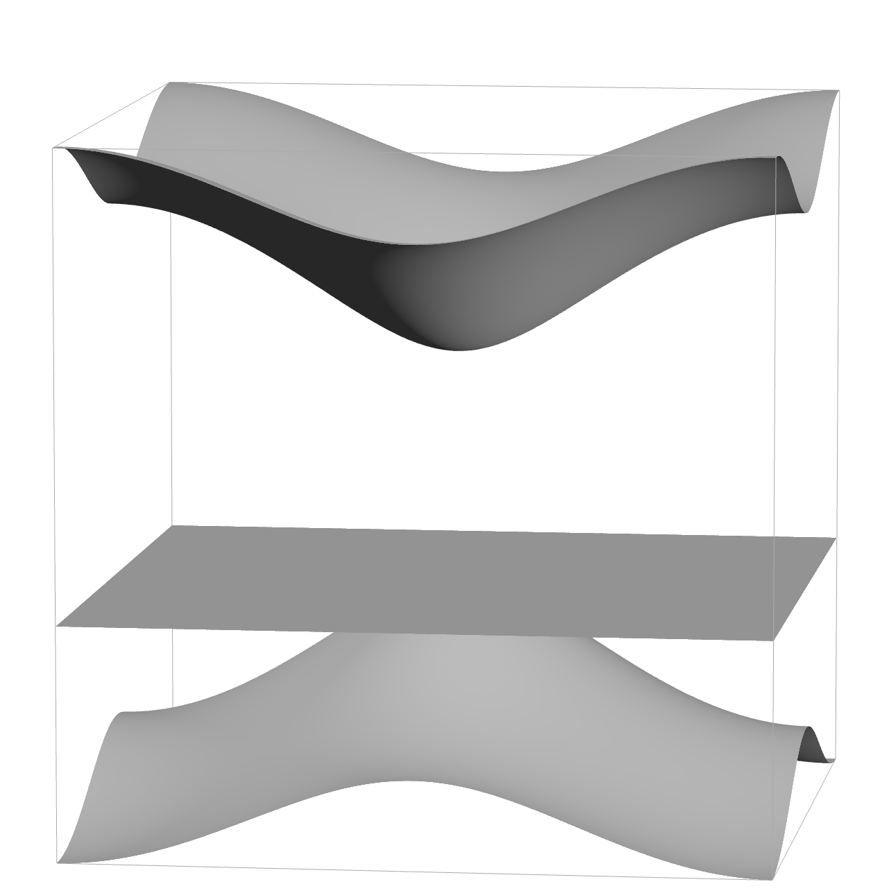
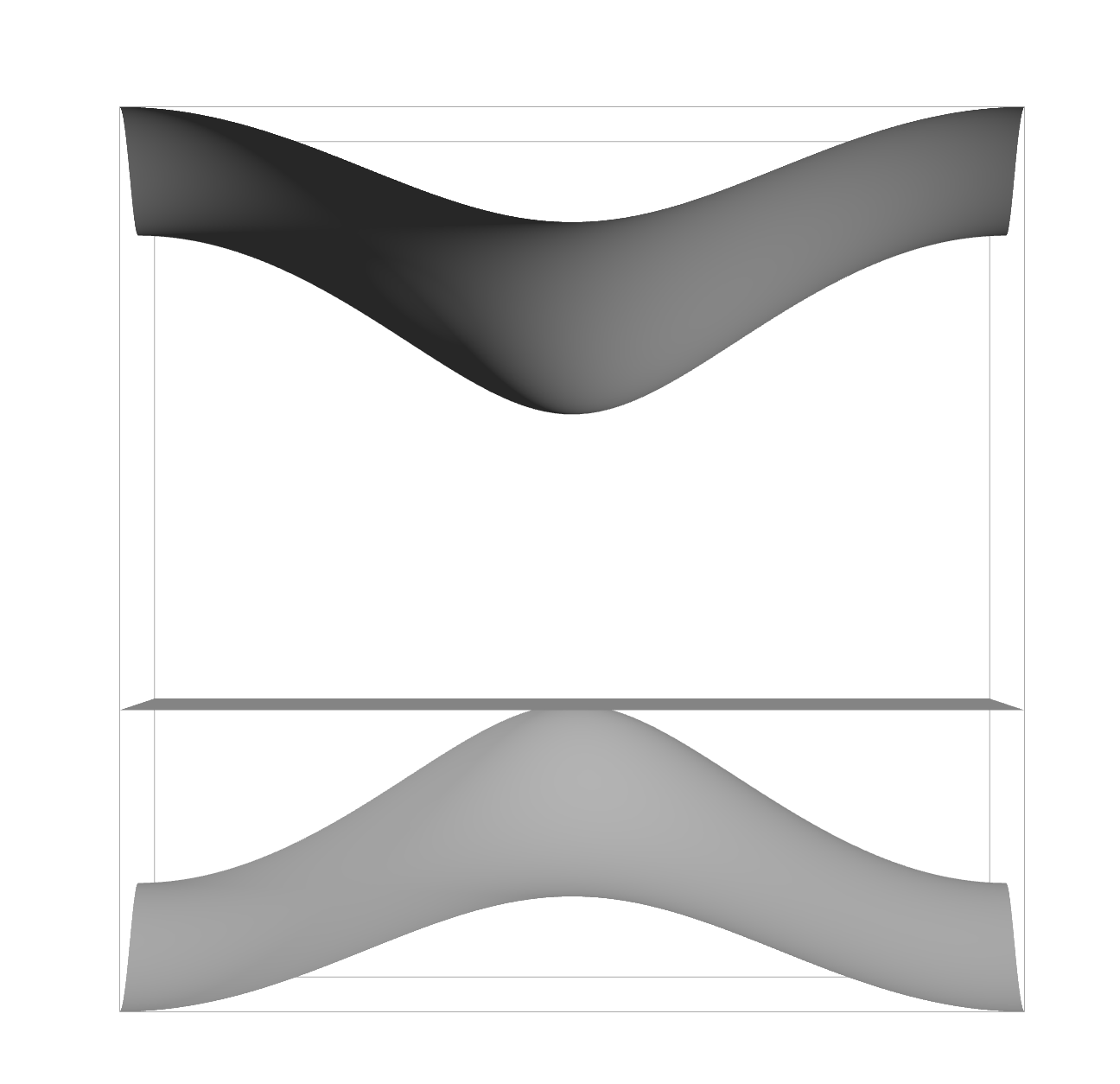
Notice that from the particular form of $h_{0}(\xi)+m$, that can be obtained directly from Equation˜5, we can check that $\operatorname{Ker}(h_{0}+m)\leq\mathcal{H}_{\mathcal{A}}$. Indeed, one can prove directly that $\operatorname{Ker}(H_{0}+m)\leq\{\mathbf{0}\}\times\ell^{2}(A)$ by constructing for each $\mu\in\mathbb{Z}^{n}$ a closed path over which we define a cochain alternating the values $1$ and $-1$, see [MPR23, Sec. 2] for an explicit construction for the $\mathbb{Z}^{2}$ case. We stress that the flat bands of discrete periodic graphs are known to generate finitely supported eigenfunctions [Kuc91].

Given the Hilbert spaces $\mathcal{H}_{1}$ and $\mathcal{H}_{2}$, we denote by $\mathfrak{S}_{\infty}(\mathcal{H}_{1},\mathcal{H}_{2})$ the class of compact operators from $\mathcal{H}_{1}$ to $\mathcal{H}_{2}$. When $\mathcal{H}_{1}=\mathcal{H}_{2}=\mathcal{H}$ we will just write $\mathfrak{S}_{\infty}(\mathcal{H})$. For $K=K^{*}\in\mathfrak{S}_{\infty}(\mathcal{H})$ and $s>0$ we set

$$n_{\pm}(s;K):=\operatorname{Rank}\mathds{1}_{(s,\infty)}(\pm K)\ .$$

Thus, the functions $n_{\pm}(\cdot;K)$ are respectively the counting functions of the positive and negative eigenvalues of the operator $K$. For $K\in\mathfrak{S}_{\infty}(\mathcal{H}_{1},\mathcal{H}_{2})$ we define

$$n_{*}(s;K):=n_{+}(s^{2};K^{*}K),\quad s>0;$$

thus $n_{*}(\cdot;K)$ is the counting function of the singular values of $K$ which, when ordered non–increasingly, we denote by $\{s_{j}(K)\}$. Let $K_{j}$, $j=1,2$ be self-adjoint compact operators. For $s_{1},s_{2}>0$, we have the Weyl inequalities (see e.g. [BS87, Theorem 9.2.9])

(18)

$$n_{\pm}(s_{1}+s_{2};K_{1}+K_{2})\leq n_{\pm}(s_{1};K_{1})+n_{\pm}(s_{2};K_{2})\ .$$

If instead we only have $\{K_{1},K_{2}\}\subset\mathfrak{S}_{\infty}(\mathcal{H}_{1},\mathcal{H}_{2})$ the Ky Fan inequality (see e.g. [BS87, Subsection 11.1.3]) gives

(19)

$$n_{*}(s_{1}+s_{2};K_{1}+K_{2})\leq n_{*}(s_{1};K_{1})+n_{*}(s_{2};K_{2})\ .$$

Further, for $0<p<\infty$ we define the class of compact operators $\mathfrak{S}_{p,w}$ by

$$\mathfrak{S}_{p,w}:=\{K\in\mathfrak{S}_{\infty}:s_{j}(K)=O(j^{-1/p})\}\ ,$$

together with the quasi-norm

$$||K||_{p,w}:=\sup_{j}\{j^{1/p}s_{j}(K)\}=\left(\sup_{s>0}\{s^{p}n_{*}(s;K)\right)^{1/p}$$

that satisfies the "weakened triangle inequality"

$$||K_{1}+K_{2}||_{p,w}\leq 2^{1/p}(||K||_{p,w}+||K||_{p,w})$$

and the "weakened Hölder inequality"

(20)

$$||K_{1}K_{2}||_{r,w}\leq c(p,q)||K_{1}||_{p,w}||K_{2}||_{q,w}\ ,$$

for $r^{-1}=p^{-1}+q^{-1}$ and $c(p,q)=(p/r)^{1/p}(q/r)^{1/q}$ (see [BS87, Chapter 11]).

Finally, consider the set $l_{p,w}$ of functions $v:\mathbb{Z}^{n}\to\mathbb{C}$ such that

$$\#\{\mu\in\mathbb{Z}^{n}:|v(\mu)|>\lambda\}=O(\lambda^{-p})\ .$$

Let us finish this section by considering the following result, which is a particular case of [BKS91, Theorem 4.8(ii)]

In this section we will use the notation

$$\mathcal{N}((a,b);T):=\operatorname{Rank}\mathds{1}_{(a,b)}(T),$$

where $a<b$ and $T$ is a self-adjoint operator without essential spectrum in $(a,b)$. Following the approach coming from the study of magnetic Schrödinger operators, our aim is to study $PVP$ where $P$ stands for the projection on the flat band, i.e.,

(21)

$$P:=\mathds{1}_{\{-m\}}(H_{0})\ .$$

Now, set $P^{\perp}:=I-P$ and for $\kappa>0$ define

$$H_{\kappa}^{\pm}:=H_{0}+P(V\pm\kappa|V|)P+P^{\perp}(V\pm\kappa^{-1}|V|)P^{\perp}$$

Then, by [PR11, Lemma 4.2]

(22)

$$H_{\kappa}^{-}\leq H\leq H_{\kappa}^{+}.$$

Then, arguing as in the proof of [PR11, Theorem 4.1(ii)] we obtain that:

	$\displaystyle\pm\mathcal{N}(\lambda)\leq$	$\displaystyle\pm\mathcal{N}((-m+\lambda,0);-mP+P(V\pm\kappa|V|)P)$
(23)			$\displaystyle\pm\mathcal{N}((-m+\lambda,0);P^{\perp}(H_{0}+(V\pm\kappa^{-1}|V|))P^{\perp})+O(1).$

In the next Lemma we treat the second term on the right of Equation˜23, showing that the perturbation $V$ interacts with the complement of the degenerated eigenspace only at a lesser order.

From Eqs.˜23 and 4.3

(24)

$$\pm\mathcal{N}(\lambda)\leq\pm\mathcal{N}((\lambda,m);P(V\pm\kappa|V|)P)+o(\lambda^{-n/\gamma}),\quad\lambda\downarrow 0\ .$$

Then, we are led to study the distribution of positives eigenvalues of the compact operator $P(V\pm\kappa|V|)P$.

For ease of notation, for any $\kappa>0$ we define $T_{\kappa}^{\pm}$ in $\mathfrak{S}_{\infty}(\mathcal{H})$ by

$$T^{\pm}_{\kappa}:=\mathscr{U}P(V\pm\kappa|V|)P\mathscr{U}^{*}=M\mathscr{U}(V\pm\kappa|V|)\mathscr{U}^{*}M\ .$$

References

• [AT15] Colette Anné and Nabila Torki-Hamza “The Gauss-Bonnet operator of an infinite graph” In Anal. Math. Phys. 5.2, 2015, pp. 137–159 DOI: 10.1007/s13324-014-0090-0
• [BL13] Emil J. Bergholtz and Zhao Liu “Topological flat band models and fractional Chern insulators” In Internat. J. Modern Phys. B 27.24, 2013, pp. 1330017\bibrangessep43 DOI: 10.1142/S021797921330017X
• [BKS91] M.. Birman, G.. Karadzhov and M.. Solomyak “Boundedness conditions and spectrum estimates for the operators b(X)a(D)b(X)a(D) and their analogs” In Estimates and asymptotics for discrete spectra of integral and differential equations (Leningrad, 1989–90) 7, Adv. Soviet Math. Amer. Math. Soc., Providence, RI, 1991, pp. 85–106
• [BS70] M.. Birman and M.. Solomjak “Asymptotics of the spectrum of weakly polar integral operators” In Izv. Akad. Nauk SSSR Ser. Mat. 34, 1970, pp. 1142–1158
• [BS87] M.. Birman and M.. Solomjak “Spectral theory of selfadjoint operators in Hilbert space” Translated from the 1980 Russian original by S. Khrushchëv and V. Peller, Mathematics and its Applications (Soviet Series) D. Reidel Publishing Co., Dordrecht, 1987, pp. xv+301
• [CGJ22] Horia Cornean, Henrik Garde and Arne Jensen “Discrete approximations to Dirac operators and norm resolvent convergence” In J. Spectr. Theory 12.4, 2022, pp. 1589–1622 DOI: 10.4171/jst/438
• [GZ23] Jeffrey Galkowski and Maciej Zworski “An abstract formulation of the flat band condition”, 2023 eprint: arXiv:2307.04896
• [IT98] Akira Iwatsuka and Hideo Tamura “Asymptotic distribution of eigenvalues for Pauli operators with nonconstant magnetic fields” In Duke Math. J. 93.3, 1998, pp. 535–574 DOI: 10.1215/S0012-7094-98-09319-X
• [KTW23] Joachim Kerner, Matthias Täufer and Jens Wintermayr “Robustness of Flat Bands on the Perturbed Kagome and the Perturbed Super-Kagome Lattice” In Annales Henri Poincaré, 2023 DOI: 10.1007/s00023-023-01399-7
• [Kla83] Martin Klaus “Some applications of the Birman-Schwinger principle” In Helv. Phys. Acta 55.1, 1982/83, pp. 49–68
• [Kol+20] Alicia J. Kollár, Mattias Fitzpatrick, Peter Sarnak and Andrew A. Houck “Line-graph lattices: Euclidean and non-Euclidean flat bands, and implementations in circuit quantum electrodynamics” In Comm. Math. Phys. 376.3, 2020, pp. 1909–1956 DOI: 10.1007/s00220-019-03645-8
• [KS14] Evgeny Korotyaev and Natalia Saburova “Schrödinger operators on periodic discrete graphs” In J. Math. Anal. Appl. 420.1, 2014, pp. 576–611 DOI: 10.1016/j.jmaa.2014.05.088
• [Kuc91] P.. Kuchment “On the Floquet theory of periodic difference equations” In Geometrical and algebraical aspects in several complex variables (Cetraro, 1989) 8, Sem. Conf. EditEl, Rende, 1991, pp. 201–209
• [MPR23] Pablo Miranda, Daniel Parra and Georgi Raikov “Spectral asymptotics at thresholds for a Dirac-type operator on 2\mathbb{Z}^{2} In J. Funct. Anal. 284.2, 2023, pp. Paper No. 109743 DOI: 10.1016/j.jfa.2022.109743
• [Nak24] Shu Nakamura “Remarks on discrete Dirac operators and their continuum limits” In J. Spectr. Theory, 2024, pp. 1–15 DOI: 10.4171/JST/478
• [Par17] D. Parra “Spectral and scattering theory for Gauss-Bonnet operators on perturbed topological crystals” In J. Math. Anal. Appl. 452.2, 2017, pp. 792–813 DOI: 10.1016/j.jmaa.2017.03.002
• [PR18] D. Parra and S. Richard “Spectral and scattering theory for Schrödinger operators on perturbed topological crystals” In Rev. Math. Phys. 30.4, 2018, pp. 1850009\bibrangessep39 DOI: 10.1142/S0129055X18500095
• [Pus09] Alexander Pushnitski “Operator theoretic methods for the eigenvalue counting function in spectral gaps” In Ann. Henri Poincaré 10.4, 2009, pp. 793–822 DOI: 10.1007/s00023-009-0422-z
• [PR11] Alexander Pushnitski and Grigori Rozenblum “On the spectrum of Bargmann-Toeplitz operators with symbols of a variable sign” In J. Anal. Math. 114, 2011, pp. 317–340 DOI: 10.1007/s11854-011-0019-6
• [PS23] Alexander Pushnitski and Alexander Sobolev “Hankel operators with band spectra and elliptic functions”, 2023 eprint: arXiv:2307.09242
• [Rai90] Georgi Raikov “Eigenvalue asymptotics for the Schrödinger operator with homogeneous magnetic potential and decreasing electric potential. I. Behaviour near the essential spectrum tips” In Comm. Partial Differential Equations 15.3, 1990, pp. 407–434 DOI: 10.1080/03605309908820690
• [RS78] Michael Reed and Barry Simon “Methods of modern mathematical physics. IV. Analysis of operators” Academic Press [Harcourt Brace Jovanovich, Publishers], New York-London, 1978, pp. xv+396
• [SY23] Mostafa Sabri and Pierre Youssef “Flat bands of periodic graphs” In J. Math. Phys. 64.9, 2023, pp. Paper No. 092101\bibrangessep23 DOI: 10.1063/5.0156336
• [Sun13] Toshikazu Sunada “Topological crystallography” With a view towards discrete geometric analysis 6, Surveys and Tutorials in the Applied Mathematical Sciences Springer, Tokyo, 2013, pp. xii+229 DOI: 10.1007/978-4-431-54177-6
• [Tha92] Bernd Thaller “The Dirac equation”, Texts and Monographs in Physics Springer-Verlag, Berlin, 1992, pp. xviii+357 DOI: 10.1007/978-3-662-02753-0
• [Zwo24] Maciej Zworski “Mathematical results on the chiral models of twisted bilayer graphene” With an appendix by Mengxuan Yang and Zhongkai Tao In J. Spectr. Theory 14.3, 2024, pp. 1063–1107 DOI: 10.4171/jst/521